Prediction of Annual Rainfall Pattern Using Hidden Markov Model ...

JASEM ISSN 1119-8362 All rights reserved

Full-text Available Online at www.ajol.infoand www.bioline.org.br/ja

J. Appl. Sci. Environ. Manage. Sept. 2016 Vol. 20 (3) 617-622

Prediction of Annual Rainfall Pattern Using Hidden Markov Model (HMM) in Jos, Plateau State, Nigeria *1

LAWAL A; 1ABUBAKAR, UY; 1DANLADI, H; 2GANA, AS 1

Department of Mathematics, 2Department of Crop Production, Federal University of Technology Minna, Nigeria

ABSTRACT: A Hidden Markov Model (HMM) is a double stochastic process in which one of the stochastic processes is an underlying Markov chain, the other stochastic process is an observable stochastic process. Hidden Markov model is very influential in stochastic world because of its uniqueness, double stochastic nature and independence assumption between consecutive observations. A hidden Markov model to predict annual rainfall pattern has been presented in this paper. The model is developed to provide necessary information for the farmers, agronomists, water resource management scientists and policy makers to enable them plan for the uncertainty of annual rainfall. The model classified annual rainfall amount into three states, each with eight possible observations. The parameters of the model were estimated from the annual rainfall data of Jos, Plateau state, Nigeria for the period of 39 years (1977-2015). After which, the model was trained using Baum-Welch algorithm to attend maximum likelihood. The model is designed such that, if given any of the three rainfall states and its observation in the present year, it is possible to make quantitative prediction on how rainfall will be in the following year and in the subsequent years. The test HMM1 was able to make prediction with 75% accuracy in state and 50% accuracy in observations. The accuracy level of the model shows that, it is dependable and therefore, information from the model could be used as a guide to the farmers, agronomists, water resources management scientists and the government to plan strategies for crop production in the region. @JASEM http://dx.doi.org/10.4314/jasem.v20i3.16 Keywords: Markov model, Hidden Markov model, Transition probability, Observation probability, Crop Production, Annual Rainfall Precipitation is the falling of water in various forms on the earth from the clouds. The usual forms of precipitation are rain, snow, sleet, glaze, hail, dew and frost (Arora, 2007). The common form of precipitation in north central Nigeria is rainfall. Rainfall is a form of precipitation that occurs when water vapour in the atmosphere condense into droplets which can no longer be suspended in the air. The occurrence of rainfall is dependent upon several factors such as prevailing wind directions, ground elevation, location, within a continental mass, and location with respect to mountain ranges, all have a major impact on the possibility of precipitation (Cwanamaker, 2011).Rainfall Modelling and predictions are essential input in agricultural production and management of water resources. Bumper harvest and lean years depend largely on rainfall variability and quantity. Rainfall modelling and prediction are becoming increasingly in demand because of the uncertainty that is involved with rainfall and the dependence of agricultural production on rainfall. It is imperative to assist the farmers and the policy makers within the immediate environment with information that could be utilized to boost agricultural production and management of water resources in

Nigeria. The majority of people living in north central Nigeria are farmers and rainfall is the major source of water for growing of crops. Annual rainfall varies in Nigeria. It decreases from the south to the north, the rainfall comes late and not evenly spread across the rainy season and consequently has adverse effect on agricultural activities (Iloeje, 1981). This seasonal variation of rainfall is the focus of this research. Mathematical models had been developed using the principle of Markov that captures the onset, recession, distribution (spread) and amount of rainfall in Jos, plateau state, Nigeria. The aim of the research, is to provide such information to the farmers and the agronomists as to when rainfall will start, end, the expected amount, and the distribution (spread) in the following year and subsequent years, this will enable them plan strategies for high crop production and this information will also serves as a guide to the policy makers and water resource management scientist to plan strategies for availability of water for other purposes in the region. The research, considered the use of stochastic tool called hidden Markov model to develop a Stochastic Mathematical model that can help

*Corresponding Authors: *E-mail: [email protected]

618

Prediction of Annual Rainfall Pattern Using Hidden Markov Model

provide information to farmers for purpose of crop production. Markov Models have become popular tools in modelling hydrological processes and other processes in field of science and Technology. Abubakar et al.,(2013) have used Markov principle to formulate a four-state model in continuous time to study the annual rainfall data with respect to the annual rainfall distribution for crop production in Minna. It was observed that if it is low rainfall in a given year, it would take at most 25%, 33% and 27% of the time to make a transition to moderate rainfall also well spread, high rainfall, and moderate rainfall but not well spread respectively in the far future. Thus given the rainfall in a year, it is possible to determine quantitatively the probability of finding rainfall in other states in the following year and in the long run. The results from the model was an important information to the farmers to plan strategies for high crop production in the region. Hughes and Guttorp (1994) have developed a nonhomogeneous hidden Markov model (NHMM) to relate broad scale atmospheric circulation patterns to local rainfall. In their work, they hypothesized unobserved, discrete-valued weather states, which classified atmospheric pattern into classes that are associated with particular precipitation patterns. In this model, transition probabilities between the hidden weather states depend on observable atmospheric data. Zucchini and Guttorp (1991) applied a hidden Markov model to describe patterns of precipitation in space and time. In the construction of this model, the authors introduced unobserved climate states with them. The transitions between these climate states were assumed to follow a Markov chain, with stationary transition probabilities. Lawal et al (2014) have developed a three state Markov model in discrete state and discrete time for annual rainfall distribution in New- Bussa. The model was designed such that if given any of the three state in a given year, it is possible to determine quantitatively the probability of making transition to any other two states in the following year(s) and in the long-run. The results from the model shows that in the long-run 70% of the annual rainfall in New-Bussa will be State1, 27% will be state 2 and 3% of the annual rainfall will be State 3. The model provides information to the Crop and Fish farmers, artisanal Fishermen, the hydroelectric power generating station in region that could be utilized to boost their production. Hidden Markov model have also been applied successfully in automatic speech recognition Rabiner(1989), pattern recognition (Fink, 1989), signal processing (Vaseghi, 2006), telecommunication (Hirsch, 2001), bioinformatics (Baldi et al., 2001)

LAWAL A; ABUBAKAR, UY; DANLADI, H; GANA, AS

MATERIALS AND METHODS Study Area and Data source: The data used in this research work, were collected from the archive of the department of Geography and Planning, faculty of environment sciences, University of Jos, plateau state, Nigeria. Jos is the capital city of plateau state, it is located between Latitude 9.95030N and longitude 8.88280E. Plateau State is located in Nigeria’s middle belt. With an area of 26,899 square kilometres, the State has an estimated population of about three million people. It is located between latitude 80°24'N and longitude 80°32' and 100°38' east. The state is named after the picturesque Jos Plateau, a mountainous area in the north of the state with captivating rock formations. Bare rocks are scattered across the grasslands, which cover the plateau. The altitude ranges from around 1,200 meters (about 4000 feet) to a peak of 1,829 metres above sea level in the Shere Hills range near Jos. Hidden Markov Model:A Hidden Markov Model (HMM) is a double stochastic process in which one of the stochastic processes is an underlying Markov chain which is called the hidden part of the model, the other stochastic process is an observable stochastic process. Also a HMM can be considered as a stochastic process whose evolution is governed by an underlying discrete (Markov chain) with a finite number of states si ϵS, i=1, N, which are hidden, i.e. not directly observable (Enza and Daniele, 2007). Hidden Markov Model is characterized by the following N = number of states in the model; M = number of distinct observation symbols per state; Q = state sequence

Q = q 1, q 2 , q 3 ,......... .... q T O = o1, o 2 , o 3 .......... ...o T O = observation sequence; Transition probability matrix is

A = {aij } Observation probability matrix

B = {b j (ot )} Where b j ( o t ) = p ( o t | q t = s j ) If the observation is continuous a probability density function is used +∞

∫b (x)dx=1 j

−∞

π = {π

j

} Initial state probabilities

λ = ( A , B, π ) The overall HMM

(1)


Formulation of the Model:In this model, we consider the amount of annual rainfall as states of the HMM while onset, recession, distribution (spread) of the rainfall within a year is taken as emission of the model. As a result, we make the following assumptions (i) The transition of annual rainfall state to another state in a year is govern by Markov chain of the first order dependence, as represented by equation (2)

P{Xt+1 = j | X0 =i0,...,Xt−2 =it−2, Xt−1 =it−1, Xt =i}=P{Xt+1 = j | Xt =i}=Pij(t) (ii)

The probability of distribution of generating current observation symbol depends only on current state. That is

619

>1300mm)’ And all the possible observations within a year is for all states given below: Let A = O1 = (rainfall starts early and ends early in that year and it is well spread); B= O2 = (rainfall starts early and ends early in that year and it is not well spread); C= O3= (rainfall starts early and ends late of that year and it is well spread); D= O4 = (rainfall starts early and ends late of that year and it is not well spread); E= O5 = (2)(rainfall starts late and ends late of that year and it is well spread); F= O6 = (rainfall starts late and ends late of that year and it is not well spread; G= O7 = (rainfall starts late and ends early of that year and it is well spread); H= O8 = (rainfall starts late and ends early of that year and it is not well spread)

T

P(O | Q, λ ) = ∏ P(ot | qt , λ ) t =1

(3) (iii) Rainfall is said to start early if it starts within (January-March) (iv) Rainfall is said to start late if it starts on the month of April or beyond (v) Rainfall is said to stop early if the rainfall does not exceed the month of October of a year (vi) Rainfall is said to stop late if the rainfall exceed the month of October Let the annual rainfall be modelled by a three state Hidden Markov Model and Eight observations The states are given below State1: Low Rainfall (rainfall amount ≤ 800mm); State2: moderate Rainfall (801mm≤ rainfall amount ≤1300mm); State3: High Rainfall (Rainfall amount O

O

Making Predictions With the Model:Making prediction with the model is done along with training of the parameters of the model. The parameters of the model are initialized, then trained using Baum-Welch algorithm reported in (Hyang-Won- Lee, 2014) and (Rabiner, 1989) to attend Maximum likelihood. The forward probability of the training observation sequence is calculated from time t=1 to time T using Forward Algorithm (Rabiner, 1989). To predict the next state at time T+1 and its observation given the present state at time T, We calculate forward probability for each possible observations of the states, then sequence with highest value of the forward probability at time T+1 is taken as predicted observation and its state. The prediction is made for the next two years (time T+2, and time T+3).

O

O

O

O O O

RESULTS AND DICUSSION

State1 22

O

O O O

State2 22

State3 22

O

O

O O

O O

Testing the Reliability of the Model: In order to test the reliability of the model we divide the dataset into two sets, one training set and the other test set.We estimate the parameter of the test HMM using the rainfall data from 1977-1994, then use it to predict annual rainfall for 1995, 1996 and 1997. The test Model (HMM1)

O O

O

O O

O

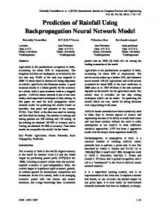
Figure.1: Transition Diagram of the Model


Transition Probability Matrix

620


0.0000 1.0000 0.0000 A = 0.0000 0.5000 0.5000 0.0000 0.5714 0.4286

( 4)

Observation probability Matrix

0.0000 0.2000 0.0000 0.0000 0.0000 0.0000 0.0000 0.0000 B = 1.0000 0.5000 0.0000 0.0000 0.0000 0.0000 0.0000 0.4000 0.0000 0.3000 0.0000 1.0000 0.0000 0.0000 1.0000 0.4000 Initial State probabilities π = [0 . 0556 0 . 5000

λ1 = ( A, B, π )

0 . 4444

]

(5)

(6)

(7)

Equation (7) is the test hidden Markov model (HMM1). After 500 iterations of the Baum Welch Algorithm using Matlab, equation (7)converged to equation (11)

 0 . 0000 1 . 0000 Aˆ =  0 . 0000 0 . 5000  0 . 0000 0 . 0000 0.0000 1.0000 0.0000 Bˆ = 0.9999 0.0000 0.0000 0.0000 0.6000 0.0000 πˆ = [ 0 0 1]

0 . 0000  0 . 5000  1 . 0000 

(8 )

0.0000 0.0000 0.0000 0.0000 0.0000 0.0000 0.0000 0.0000 0.0000 0.0001 0.0667 0.0000 0.0000 0.0667 0.2667

(9)

λ1∗ = ( Aˆ , Bˆ , πˆ ) The parameters of the HMM1 was estimated using rainfall data from 1977-1994, after 500 iterations of the Baum algorithm, λ1 converged to a new model, λ1* this new model was then used to make predictions from 1994-1997. From the prediction time series the HMM1 was in state 3(high rainfall) at time T (1994) emitted observation H (rainfall starts late and ends early of that year and it is well spread) then make transition to state 3(high rainfall) at time T+1 (1995) govern by first order Markov dependence, emitting observation B (rainfall starts early and ends early that year and it is not well spread). Similar interpretation is given to transition to state 3(high rainfall) at T+2(1996) and transition to


( 10 )

(11) state3 (high rainfall) at time T+3 (1997) both emitting observation B (rainfall starts early and ends early in that year and it is well spread). This model has 75% accuracy is state and 50% in observation in the predictions, this model was purposely developed to test for the reliability of the model.

Hidden Markov model for future Predictions (HMM2): In order to make predictions for the future years, the whole dataset (rainfall data from 1997 to 2015) was used to estimate the parameters of the model, then make predictions for 2016, 2017, and 2018

621


The Model for future predictions (HMM2): Transition Probability Matrix

0.0000 0.8000 0.200  A = 0.2100 0.4211 0.3684 0.0000 0.5000 0.5000

(12)

Observation Probability Matrix

0.0000 0.1111 0.0000 0.0000 0.0000 0.0000 0.0000 0.2500 B = 1.0000 0.4444 0.0000 0.5000 0.0000 0.0000 0.0000 0.5000 0.0000 0.4444 0.0000 0.5000 0.0000 0.0000 1.0000 0.2500 The Initial State Probabilities

π = [0 . 1282

0 . 4872

0 . 3846

]

(13)

(14)

λ2 = ( A, B, π )

(15)

After 400 iterations of the Baum Welch Algorithm, equation (15) converges to equation (19)

0.6332 0.3668  0 Aˆ = 0.7668 0.2332 0.0000  0 0.3643 0.6357

(16)

0.0000 0.0000 0.0000 0.0000 0.0000 0.0000 0.0000 Bˆ = 0.1338 0.4137 0.0000 0.1338 0.0000 0.0000 0.0000 0.0000 0.9220 0.0000 0.0000 0.0000 0.0000 0.0780 πˆ = [0 0 1] λ ∗ = ( Aˆ , Bˆ , πˆ ) 2

The parameters of the HMM2 was estimated using the whole dataset (rainfall data from 1977-2015), after 400 iteration of the Baum Welch algorithm, λ2 converged to a new model λ2*, this model was used to make predictions for annual rainfall pattern for the future years( 2016, 2017, and 2018). The prediction shows that the annual rainfall is in state 3(high rainfall) at time T(2015) with observation B(rainfall starts late and ends early of that year and it is not well spread) will make transition to state 3(high rainfall) at time T+1(2016) according to first order Markov dependence, emitting observation B(rainfall starts early and ends early in that year and it is not well spread), it then make transition to state2(moderate rainfall) at time T+2(2017) and later to


1.0000 0.3187 0.0000

(17)

( 18 )

(19 )

state1(low rainfall) at time T+3(2018) both emitting Observation B(rainfall starts early and ends early in that year and it is not well spread) Conclusion: In this paper, a hidden Markov model to predict rainfall onset, recession, distribution and amount has been presented. The test model (HMM1) was able to make prediction with 75% accuracy in states and 50% in observations,Predictions for the future years have been done. The performance by the test model shows that the model is dependable, therefore, information from this model could be used as a guide to the farmers within the region to plan strategies for high crop production. The model can also be applied in another region with little or no


modifications for crop management purposes.

production

and

water

REFERENCE Abubakar, U. Y; Lawal, A; Muhammed, A (2013).The Use of Markov Model in ContinuousTime for Prediction of Rainfall for Crop Production. IOSRJournal of Mathematics7(1):38-45 Arora, K.R (2007). Irrigation, Water Power and Water Resources Engineering. Standard Publishers Distributors, Dehi, India. Baldi, P; Brunak, Bioinformatics.ABradfordBook, Cambridge.

S The

MIT

(2001). Press,

Cwanamaker (2011).What is Rainfall and How Rainfall is created http://hubpages.com/education/What-isRainfall-and-How-is-it-Created Enza, Messina; Daniele, Toscani (2007). Hidden Markov models for scenario generation, IMAJournal of Management Mathematics 19: 379-401 Fink, G. A.(1989). Markov Models for Pattern Recognition. From Theory to Applications,Springer. Hirsch, H-G (2001). HMM adaptation for applications in telecommunication. SpeechCommunication, 34(1-2): 127-139.


622

Hughes, J.P; Guttop,P (1994). A class of Stochastic models for Relating Synoptic Atmospheric Patterns to Regional Hydrologic Phenomena. Water Res. 30: 1535-1546. Hyang-Won Lee (2014). Hidden Markov Models, Probability and Statistics Spring. P 1-18. Iloeje N.P. (1981), A New Geography of Nigeria, Longman Nigeria Limited. Lawal, Adamu; Hakimi, D; Laminu, Idris (2014). Stochastic Model of Annual Rainfall at New- Bussa. IOSRJournal of Mathematics. 10(3) 23-27. Rabiner, L.R. (1989). A tutorial on Hidden Markov Models and Selected Applications in Speech Recognition. Proc. IEEE. 77: 257-286. Vaseghi, S. V (2006). Advanced Digital Signal Processing and Noise Reduction. 4th Edition, Wiley. Zucchini, W; Guttorp, P (1991). A hidden Markov model for space-time precipitation. Water Resources Research, 27(8), 1917-1923