Hindawi Publishing Corporation Computational and Mathematical Methods in Medicine Volume 2014, Article ID 762501, 13 pages http://dx.doi.org/10.1155/2014/762501
Research Article Prediction of BP Reactivity to Talking Using Hybrid Soft Computing Approaches Gurmanik Kaur, Ajat Shatru Arora, and Vijender Kumar Jain Electrical and Instrumentation Engineering Department, Sant Longowal Institute of Engineering & Technology, Deemed University (Established by Government of India), Longowal, Sangrur District, Punjab 148106, India Correspondence should be addressed to Gurmanik Kaur;
[email protected] Received 3 June 2014; Revised 25 August 2014; Accepted 29 August 2014; Published 21 September 2014 Academic Editor: Ezequiel L´opez-Rubio Copyright © 2014 Gurmanik Kaur et al. This is an open access article distributed under the Creative Commons Attribution License, which permits unrestricted use, distribution, and reproduction in any medium, provided the original work is properly cited. High blood pressure (BP) is associated with an increased risk of cardiovascular diseases. Therefore, optimal precision in measurement of BP is appropriate in clinical and research studies. In this work, anthropometric characteristics including age, height, weight, body mass index (BMI), and arm circumference (AC) were used as independent predictor variables for the prediction of BP reactivity to talking. Principal component analysis (PCA) was fused with artificial neural network (ANN), adaptive neurofuzzy inference system (ANFIS), and least square-support vector machine (LS-SVM) model to remove the multicollinearity effect among anthropometric predictor variables. The statistical tests in terms of coefficient of determination (𝑅2 ), root mean square error (RMSE), and mean absolute percentage error (MAPE) revealed that PCA based LS-SVM (PCA-LS-SVM) model produced a more efficient prediction of BP reactivity as compared to other models. This assessment presents the importance and advantages posed by PCA fused prediction models for prediction of biological variables.
1. Introduction Accurate measurement of BP is essential in epidemiological studies, in screening programmes, in research studies, and in clinical practice to classify individuals, to ascertain hypertension related risks (coronary heart disease, stroke, and kidney failure), and to guide management. Recommendations of several international organisations including the American Heart Association (AHA) [1], British Hypertension Society (BHS) [2], and European Society of Hypertension (ESH) [3] revealed that accuracy of BP measurements is highly associated with the conditions in which the measurements are taken. The observer should be aware of the considerable variability that may occur in BP due to various factors. However, it is not always feasible to control all the factors, but we can minimize their effect by taking them into account in reaching a decision [3]. In clinical practice, talking is one of the most common measurement disturbances influencing BP measurement accuracy [4]. It can contribute to elevated BP reading, termed BP reactivity to talking, that may result in the misdiagnosis of hypertension or in overestimation of the
severity of hypertension and may lead to overly aggressive therapy. Antihypertensive treatment may be unnecessary in the absence of concurrent cardiovascular risk factors [5]. In the past few years, several studies have quantified the effect of talking on BP. Zheng et al. [6] measured BP in healthy subjects under five different conditions including resting, deeper breathing, talking, and head and arm movement and proved that SBP and DBP changed significantly in comparison to the resting condition. Le Pailleur et al. [7] explored a sharp and significant increase in SBP and DBP of hypertensive subjects while talking. Le Pailleur et al. [8] showed an instantaneous rise in SBP and DBP of treated and untreated hypertensive patients under a period of stress talking and a period of counting aloud (active periods). Zheng et al. [9] demonstrated significantly higher manual and automated MAPs with talking in healthy subjects. Lynch et al. [4] reported that verbal activity is consistently associated with marked elevations in both normotensive and hypertensive subjects. Tardy et al. [10] demonstrated that talking state increased the BP as compared to resting state of the subjects. Lynch et al. [11] described sudden extreme drop in blood pressure in both experimental and clinical situations when
2 a person is talking about or describing situations of hopelessness and helplessness. Long et al. [12] showed statistically significant increase in BP when speaking compared to when quiet. Hellmann and Grimm [13] investigated the effect of talking on subjects with one previous diastolic blood pressure reading of 90 mm Hg or more and not taking antihypertensive medicines. Blood pressure increased significantly under both talking conditions (reading neutral material for part of the procedure and reading neutral material continuously). Epidemiological studies from different populations have explored a significant correlation between BP and anthropometric characteristics [14–16]. Therefore, anthropometric variables should be considered to attain an accurate measurement of BP. However, multicollinearity between anthropometric predictor variables has also been reported, which may result in “overfitting” of the prediction model [17–19]. One approach to dealing with multicollinearity is to use PCA, a statistical approach. By using PCA the original data set can be transformed into principal components (PCs) that are orthogonal and are able to explain the maximal variance of the data without losing any information [20, 21]. Soft computing covers computational techniques that offer somewhat “inexact” solutions of very complex problems through modeling and analysis with a tolerance of imprecision, uncertainty, partial truth, and approximation. The successful applications of soft computing approaches in biomedical studies suggest that the impact of soft computing will be felt increasingly in the coming years. The fusion of a statistical and soft computing approach usually improves the training speed, enhances the robustness of the model, and reduces the calibration error. These models may aid the clinicians in the decision-making process regarding clinical admission, early prevention, early clinical diagnosis, and application of clinical therapies. In this sense, this paper focuses on the development of PCA based soft computing approaches for prediction of BP reactivity to talking, which include conventional statistical method of PCA for data preprocessing. We developed PCA based ANN (PCA-ANN), PCA based ANFIS (PCA-ANFIS), and PCALS-SVM models for prediction of BP reactivity to talking in normotensive and hypertensive subjects. The prediction accuracy of developed models was assessed and compared using statistical indices including coefficient of determination (𝑅2 ), root mean square error (RMSE), and mean absolute percentage error (MAPE) to select the model that most accurately predicts the BP reactivity. The rest of the paper is structured as follows. In Section 2, we present the details of data collection. Section 3 deals with the experimental approaches used for data analysis. Section 4 deals with the summary of results obtained. Section 5 describes the discussion and Section 6 concludes with future directions of work.
2. Data Collection A total of 40 normotensive and 30 hypertensive female subjects among the students, staff, and faculty of Sant Longowal Institute of Engineering and Technology (Deemed
Computational and Mathematical Methods in Medicine University), Longowal, District Sangrur, Punjab, India, volunteered for this study. Eligible participants had to be over 18 years of age. We excluded the subjects who were pregnant and who had arrhythmias. The institutional research committee approved the research protocol and all participants gave written informed consent before participation. A standard questionnaire was administrated to collect information on anthropometric characteristics of the participants. A specially separated room was used to conduct the study. This ensured minimal interference within the room while the tests were being carried out. The observers involved in the study were trained using the BHS’s BP measurement training materials [22]. To eliminate observer bias, BP was measured using a clinically validated (under standardized measurement conditions), newly purchased, and fully automated sphygmomanometer OMRON HEM-7203 (OMRON HEALTHCARE Co., Ltd., Kyoto, JAPAN) that uses the oscillometric method of measurement. The BP monitor is available with a small cuff (17–22 cm), medium cuff (22–32 cm), and large cuff (32– 42 cm). The appropriate size of cuff was determined from the mid-arm circumference of the subject. Subjects were advised to avoid alcohol, cigarette smoking, coffee/tea intake, and exercise for at least 30 minutes prior to their BP measurement. They were instructed to empty their bladder and sit upright with elbows on table, supported back, and feet flat on the ground, as they are the potential confounding factors. Moreover, they were asked not to talk and move during measurement [1]. After a rest period of 5 minutes [1], the measurements were performed four times repeatedly at an interval of one minute. First measurement was discarded and the average of last three measurements was taken into account. Subsequently, the same measurement protocol was repeated under talking phase during which the observer asked each subject to “tell me about your work in detail” [4]. During talking phase, the observer only talked to the subject to maintain the flow of conversation, making every possible effort to talk minimally. To improve the reliability of measurements, the subjects were examined for a week [3].
3. Experimental Methods Data were expressed as mean ± SD. A paired 𝑡-test was used to assess the difference between measurements of resting and talking conditions. 3.1. PCA. Firstly, Bartlett’s test of sphericity [23] and Kaiser Meyer Olkin (KMO) measure of sampling adequacy [24] were applied to check the suitability of data for application of PCA. Bartlett’s test of sphericity tests the null hypothesis that the correlation matrix is an identity matrix or there is no relationship between predictor variables. Consider 𝜒2 = − {[𝑁 − 1] − [
2𝐾 + 5 ]} log𝑒 |𝑅| , 6
(1)
Computational and Mathematical Methods in Medicine
3
where 𝜒 2 is chi-square, 𝑁 is sample size, 𝐾 is number of predictor variables, log𝑒 is natural log, and |𝑅| is determinant of the correlation matrix. KMO compares the magnitude of calculated correlation coefficients and partial correlation coefficients. The formula for KMO is given as follows: KMO =
∑𝑖=𝑗̸ ∑ 𝑟𝑖𝑗2 ∑𝑖=𝑗̸ ∑ 𝑟𝑖𝑗2 + ∑𝑖=𝑗̸ ∑ 𝑎𝑖𝑗2
,
w11
x1
1 w1O
2
x3
Output
h
xN
(4)
3.2. ANN. ANN’s customary architecture was composed of an input layer, an output layer, and one or more intervening layers, also referred to as hidden layers to capture the nonlinearity in data. Figure 1 shows an ANN model consisting of 𝑁 nodes in input layer, one hidden layer with ℎ hidden nodes, and an output layer with one node. Network is trained by presenting one pair of input-output vector at a time. The weighted sum of inputs calculated at 𝑡th hidden node is
Figure 1: Architecture of ANN.
Each hidden node uses a tangent sigmoid transfer function to generate an output, say 𝑍𝑡 , between 0 and 1. The outputs from each hidden nodes, along with the bias 𝑏0 on the output node, send to the output node and weighted sum becomes ℎ
NET = ∑V𝑡 𝑍𝑡 + 𝑏0 ,
where ℎ is total number of hidden nodes and V𝑡 is weight from the 𝑡th hidden node to the output node. The weighted sum NET becomes the input to the linear transfer function of the output node and the predicted output is ̂ = 𝑓 (NET) . 𝑌
(7)
And then the second phase of the BP algorithm, adjustment of the connection weights, begins. The parameters of the ANN can be determined by minimizing the following objective function in the training process: 𝑛
̂𝑗 )2 , SSE = ∑ (𝑦𝑖 − 𝑌 𝑗=1
(8)
̂𝑗 is output of the network from 𝑗th observation. where 𝑌 The sensitivity 𝑆𝑖 of the outputs to each of the 𝑖th inputs, as partial derivatives of the output with respect to the input, under the assumption that relationship of 𝑌 and 𝑋 is monotone [26], is given as 𝑆𝑖 =
ℎ ̂ 𝜕NET 𝜕𝑍𝑡 𝜕NET𝑡 ̂ 𝜕𝑌 𝜕𝑌 =∑ 𝜕𝑋𝑖 𝑡=1 𝜕NET 𝜕𝑍𝑡 𝜕NET𝑡 𝜕𝑋𝑖 ℎ
(9)
= ∑ [𝑓 (NET) V𝑡 𝑓 (NET𝑡 ) 𝑤𝑡𝑖 ]
(5)
where 𝑤𝑡𝑖 is weight on connection from the 𝑖th to the 𝑡th node, 𝑥𝑖 is input data from input node, 𝑁 is total number of input nodes, and 𝑏𝑡 is bias on the 𝑡th hidden node.
(6)
𝑡=1
𝑁
𝑖=1
who
whN
(3)
where 𝑊 is matrix of weights. To evaluate the influence of each predictor variable in the PCs, varimax rotation was used to obtain values of rotated factor loadings. These loadings represent the contribution of each predictor variable in a specific PC. The PCs used for the prediction of BP reactivity to unsupported back were obtained through multiplication of the standardized data matrix by weights (𝑊) [25].
NET𝑡 = ∑𝑤𝑡𝑖 𝑥𝑖 + 𝑏𝑡 ,
Output layer
(2)
where 𝐶 is correlation matrix of the standardized data, 𝜆 is eigenvalues, and 𝐼 is identity matrix. The weights of the variables in the PCs are then obtained by |𝐶 − 𝜆𝐼| 𝑊 = 0,
Hidden layer
x2
where ∑𝑖=𝑗̸ is sum over all variables in the matrix when variable 𝑖 ≠ 𝑗, 𝑟𝑖𝑗 is Pearson correlation coefficient between variables 𝑖 and 𝑗, and 𝑎𝑖𝑗 is partial correlation coefficient between variables 𝑖 and 𝑗. KMO index ranges, from 0 to 1, should be greater than 0.6 for the PCA to be considered appropriate. PCA is a multivariable statistical analysis technique. The objective of PCA is to remove the multicollinearity problem and reduce the number of predictor variables and transform them into PCs which are independent linear combinations of the original data set and account for the maximum possible variance of the original data set so that adequate information from the original data set can be extracted [20, 21]. The eigenvalues of the standardized matrix are calculated from |𝐶 − 𝜆𝐼| = 0,
Input layer
𝑡=1
or ℎ
𝑆̂𝑖 = ∑V𝑡 𝑤𝑡𝑖 𝑡=1
(10)
4
Computational and Mathematical Methods in Medicine x1 w1
x1 y Σ
K(x1 , xj )
x2
Σ . ..
x2
K(xp , xj )
xp Layer 1
Layer 2
Layer 3
Layer 4
Output
wp
Layer 5
Bias
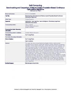
Figure 2: Architecture of ANFIS. Figure 3: Architecture of LS-SVM.
with the assumption that 𝑓 (NET) and 𝑓 (NET)𝑡 are constants. The independent variable with higher relative positive or negative sensitivity has the higher positive or negative impact on dependent variable. 3.3. ANFIS. ANFIS, a multilayer feed forward network, uses neural network learning algorithms and fuzzy reasoning to map an input space to an output space, as shown in Figure 2. It has the ability to combine the verbal power of a fuzzy system with the numeric power of a neural network. It can construct an input-output mapping based on human knowledge (if-then fuzzy rules) and stipulated inputoutput data pairs. The parameters of membership function, if-then rule exertion, and output parameters are calculated by training data set. The training algorithm is usually hybrid or back propagation. The ANFIS implements the rules of the form (𝑛) 𝑅𝑟 : If 𝑥1 is 𝐴(1) 𝑗1 . . . and 𝑥𝑛 is 𝐴 𝑗𝑛 , then 𝑦 = 𝛼0(𝑟) + 𝛼1(𝑟) ⋅ 𝑥1 + ⋅ ⋅ ⋅ + 𝛼𝑛(𝑟) ⋅ 𝑥𝑛 ,
(11)
where 𝑥1 is independent variable, 𝐴(1) 𝑗1 is a fuzzy linguistic concept, and 𝑦 is dependent variable. Input Layer (𝐿 1 ). Each unit of input layer stores parameters of membership functions to define a membership function that represents a linguistic term. Input Membership Function Layer (𝐿 2 ). Each unit of this layer represents a rule. The inputs to a unit 𝑅𝑟 ∈ 𝐿 2 are degrees of membership which are multiplied to determine the degree of fulfilment 𝜏𝑟 for the rule represented by 𝑅𝑟 . Logical Nodes (𝐿 3 ). This layer consists of a unit for each rule 𝑅𝑟 that computes relative degree of fulfilment as follows: 𝜏𝑟 𝜏𝑟 = . (12) ∑𝑅𝑖 ∈𝐿 2 𝜏𝑖 Each unit of 𝐿 3 is connected to all the rule units in 𝐿 2 . Output Membership Function Layer (𝐿 4 ). Each unit of 𝐿 4 computes the output of a rule 𝑅𝑟 as 𝑂𝑟 = 𝜏𝑟 (𝛼0(𝑟) + 𝛼1(𝑟) ⋅ 𝑥1 + ⋅ ⋅ ⋅ + 𝛼𝑛(𝑟) ⋅ 𝑥𝑛 ) .
(13)
The units 𝐿 4 are connected to all units of input layer and to exactly one unit in 𝐿 3 . Output Layer (𝐿 5 ). It computes the final output 𝑦 by adding all the outputs from 𝐿 4 [27]. 3.4. LS-SVM. LS-SVM is an extension of standard support vector machine. It converts the inequality constraints of SVM into equality ones which leads to solving a linear system instead of a quadratic problem, whose convergence speed is faster [28]. It has been widely used in estimation and approximation of function [29]. The architecture of LS-SVM is shown in Figure 3. Given a set of training data set (𝑥𝑖 , 𝑦𝑖 ) ,
𝑖 = 1, 2, . . . , 𝑙, 𝑥𝑖 ∈ 𝑅2 , 𝑦𝑖 ∈ 𝑅
(14)
with the input vector 𝑥𝑖 and the output vector 𝑦𝑖 , the regression function of least square-support vector machine, in feature space 𝐹, can be stated as 𝑦 (𝑥) = 𝑤𝑇 0 (𝑥) + 𝑏,
(15)
where 𝑤 is weight vector and 𝑏 is bias. 0(𝑥) maps the input 𝑥 into a vector in 𝐹. The model is inferred from the training data set by minimizing the cost function given below 𝛾 𝑙 1 𝑇 𝑤 𝑤 + ∑𝑒𝑖2 , 2 2 𝑖=1
(16)
subject to equality constraint 𝑦𝑖 = 𝑤𝑇 0 (𝑥𝑖 ) + 𝑏 + 𝑒𝑖 ,
(17)
where 𝑒𝑖 is error, 𝑖 = 1, 2, 3, . . . , 𝑙, and 𝛾 is regularization parameter. Solving this optimization problem in dual space leads to finding the coefficients 𝛼𝑖 and 𝑏 in the following solution: 𝑙
𝑦 (𝑥) = ∑𝛼𝑖 𝐾 (𝑥𝑖 , 𝑥) + 𝑏, 𝑖=1
where 𝐾(𝑥𝑖 , 𝑥) is kernel function.
(18)
Computational and Mathematical Methods in Medicine
5
3.5. Performance Indices Used for Model Comparison. For the comparison of developed models and selection of the optimal among them, performance of models was evaluated using 𝑅2 and RMSE and MAPE. 𝑅2 is the square of the correlation coefficient between two variables 𝑥 and 𝑦 whose 𝑛 pairs are available as follows: 𝑅2 = 1 −
2
∑𝑛𝑖=1 (𝑦𝑖 − 𝑦𝑑𝑖 )
∑𝑛𝑖=1 (𝑦𝑑𝑖 − 𝑦𝑚 )
2
.
(19)
Table 1: Descriptive characteristics of anthropometric characteristics of study sample. Anthropometric characteristic Age (year) Height (m) Weight (kg) BMI (kg/m2 ) AC (cm)
Normotensive Mean SD 23.1 1.24 1.61 0.03 55.96 7.29 21.55 2.504 26.56 2.45
Hypertensive Mean SD 42.83 6.665 1.583 0.035 62.48 10.89 23.57 3.497 26.72 2.4
RMSE is the square root of mean square error, given by following equation: 1 𝑛 2 RMSE = √ ∑(𝑦𝑖 − 𝑦𝑑𝑖 ) . 𝑛 𝑖=1
(20)
MAPE is defined as average of percentage errors, given by following equation: MAPE =
100 𝑛 𝑦𝑖 − 𝑦𝑑𝑖 ∑ , 𝑛 𝑖=1 𝑦𝑖
(21)
where 𝑛 is the number of samples, 𝑦𝑖 is the predicted value obtained from the model, 𝑦𝑑𝑖 is the actual value, and 𝑦𝑚 is the average of the actual values. The lower the RMSE and MAPE, the better the accuracy of the model in predicting the parameter. Also, the highest 𝑅2 values indicated that the model performed the best [30].
4. Results Descriptive statistics for each anthropometric characteristic is given as mean and SD in Table 1. The results of paired 𝑡-test demonstrated statistically significant higher SBP, DBP, and mean arterial pressure (MAP), (𝑃 < 0.001) in talking condition. The mean rise was found to be higher in hypertensive individuals than normotensives, as shown in Table 2. These results are consistent with the recommendations of AHA for BP measurement in humans and experimental animals [1]. Table 3 presents the Pearson’s correlation coefficients calculated for all anthropometric variables. High values of correlation coefficient (greater than 0.6) between pairs of anthropometric characteristics [31] revealed the existence of multicollinearity. Before applying PCA, Bartlett’s test of sphericity and Kaiser-Meyer-Olkin (KMO) measure of sampling adequacy were applied to determine whether PCA was suitable for data studied. The results are shown in Table 4. High value of chisquare (𝜒 2 ) for Bartlett’s test suggests that use of PCA is appropriate (𝑃 < 0.001) in normotensive and hypertensive subjects. The value of KMO is also greater than 0.6 which indicates that our sample size is enough to apply PCA [32]. The first four PCs (PC1–PC4), explaining more than 5% of total variation, as shown in Table 5, were retained for further analysis. Rotated component loadings after varimax rotation represent the extent to which the original anthropometric
characteristics are influential in forming PCs, as shown in Table 6. The bold marked loads show the highest correlation between anthropometric characteristic and corresponding component. For both normotensive and hypertensive subjects, weight and BMI were positively highly correlated with PC1 and a negative high correlation between height and PC2 was observed. Principal score values for assigned PCs were determined by using principal score coefficients. Moreover, the value of Pearson’s correlation (correlation coefficient < 0.6) between PCs, as shown in Table 7, indicates the elimination of multicollinearity effect presented in Table 3. To develop PCA based soft computing prediction models 80% of data were used for training while entire data set was used for testing. Moreover, data must be normalized to achieve more accurate predictions [38]. The predicted BP reactivity values were denormalized for comparison with the actual values. MATLAB 7.5 version was used to develop the prediction models. 4.1. PCA-ANN. To achieve the best ANN structure for BP reactivity prediction, various structures of feed-forward neural network with different number of neurons in hidden layer were investigated. Finally, with consideration of statistical indices, a structure with two hidden layers, having six nodes in each hidden layer, was developed. There were four input nodes representing the four PCs and one output node representing the BP reactivity to talking. Tangent sigmoid and linear transfer functions were used as activation functions in the hidden and output layers. Back propagation learning algorithm based on Levenberg-Marquardt technique was used [39]. Figures 4 and 5 show the scatter plot between observed and predicted values of SBP, DBP, and MAP reactivity from PCA-ANN model in normotensive and hypertensive subjects, respectively. 4.2. PCA-ANFIS. PCA-ANFIS model was developed using genfis1 with grid partition on data. Different ANFIS parameters were tested in order to achieve the perfect training and maximum prediction accuracy. Input membership functions “trapmf ” and “gauss2mf ” were used to predict SBP and DBP reactivities, respectively, in normotensive individuals, whereas membership function
6
Computational and Mathematical Methods in Medicine Table 2: Results of paired 𝑡-test.
Subjects
Mean difference ± SD 6.31 ± 2.409 5.857 ± 1.584 6.008 ± 1.231 9.634 ± 1.283 7.816 ± 1.44 8.422 ± 1.105
BP, mm Hg SBP DBP MAP SBP DBP MAP
Normotensives
Hypertensives
𝑡 16.567 23.388 30.854 41.117 29.722 41.757
12
Predicted BP reactivity to talking (mmHg)
Predicted BP reactivity to talking (mmHg)
95% CI of mean difference 5.540 to 7.081 5.350 to 6.363 5.164 to 6.402 9.154 to 10.113 7.278 to 8.354 8.009 to 8.834
11
13 PCA-ANN
11 10 9 8 7 6 5 4 3
𝑃