Prediction of Defective Software Modules Using Class Imbalance ...

Hindawi Publishing Corporation Applied Computational Intelligence and So Computing Volume 2016, Article ID 7658207, 12 pages http://dx.doi.org/10.1155/2016/7658207

Research Article Prediction of Defective Software Modules Using Class Imbalance Learning Divya Tomar and Sonali Agarwal Indian Institute of Information Technology, No. 5203, CC-3 Building, Allahabad, Uttar Pradesh 211012, India Correspondence should be addressed to Divya Tomar; [email protected] Received 17 November 2015; Accepted 19 January 2016 Academic Editor: Zhang Yi Copyright © 2016 D. Tomar and S. Agarwal. This is an open access article distributed under the Creative Commons Attribution License, which permits unrestricted use, distribution, and reproduction in any medium, provided the original work is properly cited. Software defect predictors are useful to maintain the high quality of software products effectively. The early prediction of defective software modules can help the software developers to allocate the available resources to deliver high quality software products. The objective of software defect prediction system is to find as many defective software modules as possible without affecting the overall performance. The learning process of a software defect predictor is difficult due to the imbalanced distribution of software modules between defective and nondefective classes. Misclassification cost of defective software modules generally incurs much higher cost than the misclassification of nondefective one. Therefore, on considering the misclassification cost issue, we have developed a software defect prediction system using Weighted Least Squares Twin Support Vector Machine (WLSTSVM). This system assigns higher misclassification cost to the data samples of defective classes and lower cost to the data samples of nondefective classes. The experiments on eight software defect prediction datasets have proved the validity of the proposed defect prediction system. The significance of the results has been tested via statistical analysis performed by using nonparametric Wilcoxon signed rank test.

1. Introduction Software Development Life Cycle (SDLC) consists of five phases: Analysis, Design, Implementation, Test, and Maintenance phases. These phases should be operated effectively in order to deliver bug-free and high quality software product to the end users. Developing a defect-free software product is a very challenging task due to the occurrence of unknown bugs or unforeseen deficiencies even if all the guidelines of software project development are followed carefully. Early prediction of defective software modules helps the software project manager to effectively utilize the resources such as people, time, and budget to develop high quality software [1–4]. Identifying defective software modules is a major issue of concern in the software industry which facilitates further software evolution and maintenance. Software project managers, quality managers, and software developers monitor, detect, and correct software defects in all phases of software development life cycle in order to deliver quality software on time and within budget. The quality of a software product is highly correlated with the absence or presence of

the defects [5, 6]. A software defect is an error or deficiency in a software process which occurs due to incorrect programming logic, miscommunication of requirements, lack of coding experience, poor software testing skill, and so forth. Defective software modules generate wrong output and lead to a poor quality software product which further increases the development and maintenance cost and is responsible for customer dissatisfaction [1, 2]. In last two decades researchers have focused on software defect prediction problem by applying several statistical and machine learning techniques. The software defect data suffers from the class imbalance problem due to the skewed distribution of defective and nondefective software modules [7–11]. Mostly machine learning algorithms consider equal distribution of data samples in each class and assume the misclassification cost of each class is equally important. However, the misclassification cost of data samples of minority class is higher than that of the data samples of majority class in most cases [12]. In case of the software defect prediction, predicting the defective software module as nondefective one can increase the cost of maintenance and for the opposite case in which nondefective

2 module is considered as defective can involve unnecessary testing activities. But the latter is generally more acceptable than the former. Hence, the objective of this research work is to consider the different misclassification cost of each class for the effective prediction of defective software modules. Software defect prediction problem requires a binary classifier as it is a two-class classification problem. In recent years, many nonparallel hyperplane Support Vector Machine (SVM) classifiers have been proposed by the researchers for binary classification [13–15]. For example, Mangasarian and Wild proposed a Generalized Eigenvalue Proximal Support Vector Machine (GEPSVM), which is the first nonparallel hyperplane classifier and it aims to find a pair of nonparallel hyperplane in such a way that each hyperplane is nearest to one of the two classes and as far as possible from the other class [16]. GEPSVM shows excellent performance with several benchmark datasets especially with the “Cross-Planes” dataset. Later, by utilizing the concept of traditional SVM and GEPSVM, Jayadeva et al. proposed a nonparallel hyperplane based novel binary classifier, named as TWSVM [13]. TWSVM has shown better performance as compared to Support Vector Machine (SVM) and other classifiers not only in terms of predictive accuracy but also in terms of time [13, 14]. For equally distributed classes, the training process of TWSVM is four times faster than that of SVM as it solves two smaller Quadratic Programming Problems (QPPs) instead of a complex QPP as in SVM. TWSVM seeks two nonparallel hyperplanes one for each class in such a way that each hyperplane remains within the close affinity of its corresponding class while being as far as possible from the other class. Although TWSVM classifier is faster than that of conventional SVM, yet it involves solving of two QPPs which is a complex process. Hence, Arun Kumar and Gopal proposed a binary classifier referred to as Least Squares Twin Support Vector Machine (LSTSVM) which solves two linear equations rather than two QPPs as in TWSVM [17]. It is the least square variant of Twin Support Vector Machine (TWSVM). LSTSVM has shown its effectiveness over TWSVM in terms of better generalization ability and lesser computational time. Therefore, this research work has adopted LSTSVM classifier for the defect prediction in software modules. This study takes the misclassification cost issue into account and proposes a Weighted Least Squares Twin Support Vector Machine classifier to develop a software defect prediction system that considers misclassification cost for each class. Experiments on eight software defect prediction datasets taken from PROMISE repository demonstrate the superiority of our proposed system over existing approaches, including Support Vector Machine (SVM), Cost-Sensitive Neural Network (CBNN), weighted Naive Bayes (NB), Random Forests (RF), Logistic Regression (LR), 𝑘-Nearest Neighbor (𝑘-NN), Bayesian Belief Network (BBN), C4.5 Decision Tree, and Least Squares Twin Support Vector Machine (LSTSVM). The effectiveness of the proposed software defect prediction system has also been analyzed by using nonparametric Wilcoxon signed rank hypothesis tests. The statistical inferences are made from the observed difference in the geometric mean.

Applied Computational Intelligence and Soft Computing The paper is organized into five sections. Section 2 summarizes the related work in the field of software defect prediction and class imbalance learning. Section 3 discusses the proposed software defect prediction approach. Results of experiment are presented and discussed in Section 4 and conclusion is drawn in Section 5.

2. Related Work 2.1. Class Imbalance Learning. In imbalanced data distribution, one class contains large number of data samples (majority class) as compared to the other class (minority class). Traditional classification algorithms assume balanced distribution of data samples among classes. The degree of imbalance varies from one problem domain to another and the correct class prediction of data samples in an unusual class becomes more important than the contrary case. In the software defect prediction problem the cases of defective software modules are less as compared to nondefective software modules. For such type of problem, software developers take more interest in the correct identification of defective software modules. The failure to identify defective software modules can degrade the software quality. Therefore, a software defect predictor could be beneficial if it correctly recognizes the defective software modules. Class imbalanced learning is the process of learning from the imbalanced datasets [18]. The challenge of imbalanced data learning is that the unusual class cannot draw equal attention to the learning algorithm as compared to the majority class. For imbalanced dataset, the learning algorithm generates specific or missing classification rules for the unusual class [18–20]. These rules cannot be generalized well for the unseen data and thus are not appropriate for the future prediction. Various solutions have been recommended by the researchers to handle class imbalance problem-data level, algorithmic level, and cost-sensitive solutions. In data level solutions, the training data is manipulated to rebalance the distribution of data among classes for the purpose of rectifying the effect of class imbalance by using different resampling techniques such as random oversampling, random undersampling, SMOTE, informed undersampling, and cluster based sampling [20–27]. Data level solutions are more versatile in nature as they are independent of the learning algorithms. In algorithmic level solutions, the learning algorithms modify their training mechanism with the objective to achieve better accuracy on the minority class. One-class learning approaches such as REMED and RIPPER are used to predict the data samples of minority class [28]. Ensemble learning approaches have been used by the researchers for imbalance data handling. In this approach, a set of classifiers are used for learning and their outputs are combined in order to predict the class of new data samples. Boosting, Random Forest, AdaBoost. NC, SMOTEBoost, and so forth are examples of ensemble learning approaches [29]. Cost-sensitive learning methods consider different misclassification cost for different classes in such a way that the data samples of minority class get importance. Cost-Sensitive Decision Tree, Cost-Sensitive Neural Network, and Cost-Sensitive Boosting

Applied Computational Intelligence and Soft Computing methods such as Adacost are some approaches which are proposed by the researchers to handle the class imbalance learning problem [30–33]. Cost functions have also been combined with Support Vector Machine and Bayesian classifiers. 2.2. Software Defect Prediction. Researchers are taking great interest in software defect prediction problem using statistical and machine learning algorithms such as Neural Network, Support Vector Machine, Naive Bayes, Random Forest, Case Based Reasoning, Logistic Regression, and Association Rule Mining [34–40]. K. O. Elish and M. O. Elish investigated the capability of Support Vector Machine in predicting defective software modules and analyzed its performance against some statistical and machine learning approaches on four NASA datasets [37]. Czibula et al. developed a system to identify the defective software modules using relational association rule mining which is an extension of association rules [38]. Association rules are used to determine the different types of relations between metrics for defect prediction. Challagulla et al. have evaluated the performance of various machine learning approaches and statistical models on four software defect prediction datasets taken from NASA repository for predicting software quality [41]. From experiments, it was analyzed that the combination of 1-rule classification and instance based learning incorporation with consistency based subset evaluation approach achieved the highest defect predictive accuracy as compared to the other methods. Guo et al. proposed Random Forests, which is an extension of Decision Tree, for identifying the defective software modules [39]. They have performed experiment on five case studies based on NASA datasets and compared the performance of their proposed methodology with statistical and machine learning approaches of WEKA and See5 machine learning packages. They concluded that the Random Forest algorithm has produced higher defect prediction rate as compared to the other approaches. Moeyersoms et al. used Data Mining approaches such as Random Forest, Support Vector Regression, C4.5, and Regression Tree [42]. They have applied ALPA rule extraction technique to improve the rule sets in terms of accuracy, fidelity, and recall. Okutan and Yıldız developed a software defect prediction model by using Bayesian Network [43]. This model determines the probabilistic influential relationships of software metrics with defect-prone software modules. Bayesian Network is one of the most widely used approaches to analyze the effect of object-oriented metrics on the number of defects [43–48]. Pai and Dugan performed experiment on KC1 project taken from NASA repository using Bayesian Network [47]. Fenton et al. used Bayesian Network to predict the defect, quality, and risk of software system [48]. They have analyzed the influence of information variables such as test effectiveness and defect present on target variable defects detected. Catal and Diri have investigated the effect of dataset size, metrics, and feature selection on the prediction of defective software modules [49]. They have conducted experiments on five datasets and analyzed that the Random Forest (RF) algorithm obtained better performance on large datasets while Naive Bayes performed better on small datasets as compared to

3 RF. Again they have used Artificial Immune System (AIS) algorithm to analyze the effect of metrics set. Artificial Immune Recognition Systems (AIRS2Parallel) perform better with the method level metrics while Immunos2 algorithm shows better results with class-level metrics. They have found that the algorithm is more important component of software defect prediction than the metrics suite. Apart from these basic classification approaches, several optimization approaches such as Genetic Algorithm, Particle Swarm Optimization (PSO), and Ant Colony Optimization (ACO) have also been applied to the software defect prediction problem [50–52]. The imbalance distribution of defective and nondefective software modules leads to the poor performance of machine learning approaches. To balance the distribution of data samples between classes, various solutions such as oversampling and undersampling methods have been applied by the researchers. Arar and Ayan proposed a Cost-Sensitive Neural Network based defect prediction system with the objective to handle class imbalance problem [53]. Artificial Bee Colony algorithm was used to find the optimal weights. They have investigated the performance of their proposed approach on five publically available datasets taken from NASA repository. Zheng considered different misclassification costs and developed a software defect prediction model by using Cost-Sensitive Boosting Neural Network [8]. Khoshgoftaar and Gao also studied the impact of data sampling and feature selection on software defect prediction datasets [10, 54]. They used wrapper based feature selection approach to select relevant features and random undersampling to reduce the negative impact of imbalanced data on the performance of software defect prediction model. Wang and Yao investigated the impact of imbalanced data on the software defect prediction learning models [7]. They have performed experiments on ten publically available datasets taken from PROMISE repository with different types of class imbalance learning approaches such as resampling, ensemble approach, and threshold moving. From the experiment, it was found that the AdaBoost.NC has shown better performance as compared to the other approaches. Jing et al. employed dictionary learning approach and proposed a costsensitive discriminative dictionary learning (CDDL) based software defect prediction model. They have analyzed the performance of their proposed model on ten NASA datasets [55]. Apart from these researches, various studies have been done on predicting the software defect using Data Mining techniques. Researchers have also analyzed the impact of metrics on identifying defect-prone software modules. They have focused on the selection of relevant metrics which are useful for defect prediction [52, 56–62]. From the literature, we have analyzed that the Data Mining plays crucial role in predicting software defect. The datasets which are used for defect prediction are highly imbalanced in nature as the number of defective software modules is usually less than the nondefective software modules. Therefore, this research work focuses on the imbalance nature of software defect prediction dataset in order to get effective results.

4

Applied Computational Intelligence and Soft Computing

3. Weighted Least Squares Twin Support Vector Machine

to determine the following two nonparallel hyperplanes:

Only few researches have considered the misclassification cost of defective and nondefective software modules. This research work has used Weighted Least Squares Twin Support Vector Machine (WLSTSVM) to develop the effective software defect prediction model in which different misclassification cost or weight is assigned to each class according to its sample distribution. Let the training dataset contain “𝑛” data samples {(𝑥1 , 𝑦1 ), (𝑥2 , 𝑦2 ), . . . , (𝑥𝑛 , 𝑦𝑛 )}, where 𝑥𝑖 ∈ 𝑅𝑑 , 𝑖 = 1, 2, . . . , 𝑛, denotes feature vector and 𝑦𝑖 ∈ {1, 2} represents corresponding class label. Suppose the size of class 1 and class 2 is 𝑛1 and 𝑛2 correspondingly, where 𝑛 = 𝑛1 + 𝑛2 . Let matrices 𝐴 1 ∈ 𝑅𝑛1 ×𝑑 and 𝐴 2 ∈ 𝑅𝑛2 ×𝑑 consist of data samples of class 1 and class 2, respectively. The appropriate selection of cost is an important issue of consideration. The weight or misclassification cost is determined for each class according to the following formula: 𝑝𝑖 =

𝑛𝑖 , where 𝑖 = 1, 2. 𝑛

(1)

The following conclusions can be drawn from the abovementioned formula: (1) Cost lies within 0 to 1 range, that is, 𝑝𝑖 ∈ (0, 1) so that the classifier could be trained with convergence. (2) Costs are normalized (∑2𝑖=1 𝑝𝑖 = 1) without loss of generality. (3) Lower misclassification cost is assigned to the majority class while minority class receives higher misclassification cost.

𝑓1 = (𝑤1 ⋅ 𝑥) + 𝑏1 = 0, 𝑓2 = (𝑤2 ⋅ 𝑥) + 𝑏2 = 0.

Here, 𝑤1 and 𝑤2 are two normal vectors to the hyperplanes and 𝑏1 and 𝑏2 are bias terms. 𝑐1 and 𝑐2 represent nonnegative penalty parameters. 𝑒1 ∈ 𝑅𝑛1 and 𝑒2 ∈ 𝑅𝑛2 are the vectors of 1’s and 𝜉 ∈ 𝑅𝑛2 , 𝜂 ∈ 𝑅𝑛1 are slack variables. 𝑊1 ∈ 𝑅𝑛2 ×𝑛2 and 𝑊2 ∈ 𝑅𝑛1 ×𝑛1 represent the diagonal matrix containing misclassification cost for the data samples of class 2 and class 1, respectively, according to (1). The first term of the objective function as indicated in (2) measures the squared sum distances of the data samples of class 1. The minimization of it keeps the hyperplane in the close proximity with class 1. The second term of the objective function minimizes the misclassification error due to the data samples of class 2. Thus, in this way the hyperplane is kept near the data samples of class 1 and as far as possible from the data samples of class 2. The Lagrangian function corresponding to (2) is given by 𝐿 (𝑤1 , 𝑏1 , 𝜉, 𝛼) =

min (𝑤1 , 𝑏1 , 𝜉) s.t. min (𝑤2 , 𝑏2 , 𝜂) s.t.

1 󵄩󵄩 󵄩2 𝑐 𝑇 󵄩𝐴 𝑤 + 𝑒 𝑏 󵄩󵄩 + 1 𝜉 𝑊1 𝜉 2 󵄩 1 1 1 1󵄩 2

(2)

(𝐴 1 𝑤2 + 𝑒1 𝑏2 ) + 𝜂 = 𝑒1

(3)

(5)

− 𝛼 (− (𝐴 2 𝑤1 + 𝑒2 𝑏1 ) + 𝜉 − 𝑒2 ) = 0. Here, 𝛼 > 0 is a Lagrangian multiplier. Following KarushKuhn-Tucker (KKT) necessary and sufficient optimality conditions are determined by differentiating (5) with respect to 𝑤1 , 𝑏1 , 𝜉, and 𝛼: 𝜕𝐿 = 𝐴𝑇1 (𝐴 1 𝑤1 + 𝑒1 𝑏1 ) + 𝐴𝑇2 𝛼 = 0, 𝜕𝑤1

(6)

𝜕𝐿 = 𝑒1𝑇 (𝐴 1 𝑤1 + 𝑒1 𝑏1 ) + 𝑒2𝑇 𝛼 = 0, 𝜕𝑏1

(7)

𝜕𝐿 = 𝑐1 𝑊1 𝜉 − 𝛼 = 0, 𝜕𝜉

(8)

𝜕𝐿 = (𝐴 2 𝑤1 + 𝑒2 𝑏1 ) − 𝜉 + 𝑒2 = 0. 𝜕𝛼

(9)

Equations (6) and (7) lead to 𝑤1 𝑋2𝑇 𝑋1𝑇 [ 𝑇 ] [𝑋1 𝑒1 ] [ ] + [ 𝑇 ] 𝛼 = 0. 𝑏1 𝑒1 𝑒2

(10)

𝑤

Let 𝑢1 = [ 𝑏11 ], 𝐵1 = [𝐴 1 𝑒1 ], and 𝐵2 = [𝐴 2 𝑒2 ]. With these notations, (10) can be rewritten as 𝐵1𝑇 𝐵1 𝑢1 + 𝐵2𝑇 𝛼 = 0,

− (𝐴 2 𝑤1 + 𝑒2 𝑏1 ) + 𝜉 = 𝑒2 , 1 󵄩󵄩 󵄩2 𝑐 𝑇 󵄩󵄩𝐴 2 𝑤2 + 𝑒2 𝑏2 󵄩󵄩󵄩 + 2 𝜂 𝑊2 𝜂 2 2

1 󵄩󵄩 󵄩2 𝑐 𝑇 󵄩󵄩𝐴 1 𝑤1 + 𝑒1 𝑏1 󵄩󵄩󵄩 + 1 𝜉 𝑊1 𝜉 2 2 𝑇

Linear and nonlinear WLSTSVM classifier is formulated as follows. 3.1. Linear WLSTSVM. Least Squares Twin Support Vector Machine (LSTSVM), proposed by Arun Kumar and Gopal, is a binary classifier which classifies the data samples of two classes by generating hyperplane for each class [17]. The hyperplanes are constructed in such a way that the data samples of each class lie in the close proximity of its corresponding hyperplane while maintaining clear separation from other hyperplanes. For each new data sample, its distance is calculated from each hyperplane and the data sample is assigned into the class which lies closer to it. Weighted Least Squares Twin Support Vector Machine is obtained by adding weight or misclassification cost to the formulation of LSTSVM according to (1). Linear WLSTSVM solves the following two objective functions:

(4)

−1

or 𝑢1 = − (𝐵1𝑇 𝐵1 ) 𝐵2𝑇 𝛼.

(11)

The solution of the above equation requires the inverse 𝐵1𝑇 𝐵1 . However, sometimes it is not possible to determine the inverse of it due to ill-conditioned matrix. To avoid this situation, a regularization term 𝛿𝐼 may be added to the 𝐵1𝑇 𝐵1 .

Applied Computational Intelligence and Soft Computing Here, 𝛿 > 0 and 𝐼 is an identity matrix of suitable dimension. Equation (11) can be rewritten as −1

𝑢1 = − (𝐵1𝑇 𝐵1 + 𝛿𝐼) 𝐵2𝑇 𝛼.

(12)

5 Here, “𝐾” is an appropriately chosen kernel function and 𝐷 = 𝑇 [𝐴 1 𝐴 2 ] . Nonlinear WLSTSVM classifier is constructed as min (𝜇1 , 𝛾1 , 𝜉)

Lagrangian multiplier is determined by (8), (9), and (11) as −1

−1 𝑊 −1 𝛼 = [ 1 + 𝐵2 (𝐵1𝑇 𝐵1 ) 𝐵2𝑇 ] 𝑒2 . 𝑐1

(13)

1 󵄩󵄩 󵄩2 𝑐 𝑇 󵄩󵄩𝐴 2 𝑤2 + 𝑒2 𝑏2 󵄩󵄩󵄩 + 2 𝜂 𝑊2 𝜂 2 2

min (𝜇2 , 𝛾2 , 𝜂)

(14)

− 𝛽𝑇 ((𝐴 1 𝑤2 + 𝑒1 𝑏2 ) + 𝜂 − 1) = 0. Here, 𝛽 > 0 is a Lagrangian multiplier. The hyperplane parameters corresponding to class 2 are obtained by solving the above equation (14) as −1

𝑢2 = (𝐵2𝑇 𝐵2 ) 𝐵1𝑇 𝛽,

(15) −1

−1 𝑊 −1 𝛽 = [ 2 + 𝐵1 (𝐵2𝑇 𝐵2 ) 𝐵1𝑇 ] 𝑒1 . 𝑐2

(16)

Hyperplane parameters are obtained using (11) and (15) which are further used to determine nonparallel hyperplanes, one for each class. A class is assigned to new data sample depending on which plane lies closest to it. The decision function for class evaluation is defined as 󵄨󵄨 󵄨 󵄨𝑤 ⋅ 𝑥 + 𝑏 󵄨󵄨 (17) class 𝑖 = arg min 󵄨 𝑖 󵄩󵄩 󵄩󵄩 𝑖 󵄨 . 𝑖=1,2 󵄩󵄩𝑤𝑖 󵄩󵄩 Algorithm 1. (1) Define weight matrix for each class (defective or nondefective) using (1). (2) Obtain matrices 𝐵1 = [𝐴 1 𝑒1 ] and 𝐵2 = [𝐴 2 𝑒2 ] where matrices 𝐴 1 and 𝐴 2 comprise the software modules of defective and nondefective classes or vice versa. (3) Select the penalty parameters on validation basis. (4) Determine hyperplane parameters using (12) and (15) which are further used to determine the hyperplane for each class. (5) For new software module its class (either it is defective or not) is determined by using decision function as mentioned by (17). 3.2. Nonlinear WLSTSVM. Nonlinear WLSTSVM is obtained by using kernel trick. Kernel function maps the data samples into higher-dimensional feature space in order to make easier separation. WLSTSVM classifier generates the following kernel surfaces in that space instead of hyperplanes: 𝐾 (𝑥, 𝐷𝑇 ) 𝜇1 + 𝛾1 = 0, 𝐾 (𝑥, 𝐷𝑇 ) 𝜇2 + 𝛾2 = 0.

− (𝐾 (𝐴 2 , 𝐷𝑇 ) 𝜇1 + 𝑒2 𝛾1 ) + 𝜉 = 𝑒2 ,

s.t.

In the same way, Lagrangian function of (3) is obtained as 𝐿 (𝑤2 , 𝑏2 , 𝜂, 𝛽) =

1 󵄩󵄩 󵄩2 󵄩󵄩𝐾 (𝐴 1 , 𝐷𝑇 ) 𝜇1 + 𝑒1 𝛾1 󵄩󵄩󵄩 󵄩 󵄩 2 𝑐 + 1 𝜉𝑇 𝑊1 𝜉, 2

(18)

1 󵄩󵄩 󵄩2 󵄩󵄩(𝐴 , 𝐷𝑇 ) 𝜇2 + 𝑒2 𝛾2 󵄩󵄩󵄩 󵄩 2󵄩 2 𝑐 + 2 𝜂𝑇 𝑊2 𝜂, 2

s.t.

(19)

(𝐾 (𝐴 1 , 𝐷𝑇 ) 𝜇2 + 𝑒1 𝛾2 ) + 𝜂 = 𝑒1 .

Let 𝐶1 = [𝐾(𝐴 1 , 𝐷𝑇 )𝑒1 ] and 𝐶2 = [𝐾(𝐴 2 , 𝐷𝑇 )𝑒2 ]. The kernel generated surface parameters are obtained as 𝜇1 −1 [ ] = − (𝐶1𝑇 𝐶1 ) 𝐶2𝑇 𝛼, 𝛾1

(20) −1

𝛼=[

−1 𝑊1 −1 + 𝐶2 (𝐶1𝑇 𝐶1 ) 𝐶2𝑇 ] 𝑒2 , 𝑐1

𝜇2 −1 [ ] = (𝐶2𝑇 𝐶2 ) 𝐶1𝑇 𝛽, 𝛾2

(21)

(22) −1

𝛽=[

−1 𝑊2 −1 + 𝐶1 (𝐶2𝑇 𝐶2 ) 𝐶1𝑇 ] 𝑒1 . 𝑐2

(23)

These parameters generate kernel surfaces and the class is assigned to new data sample depending on its distance from the kernel surface. The decision function is defined as 󵄨󵄨 󵄨 󵄨󵄨𝐾 (𝑥, 𝐷𝑇 ) 𝜇𝑖 + 𝛾𝑖 󵄨󵄨󵄨 󵄨 󵄨. (24) class 𝑖 = arg min 󵄩󵄩󵄩𝜇𝑖 󵄩󵄩󵄩 𝑖=1,2 󵄩 󵄩 The algorithm of nonlinear WLSTSVM classifier is similar to that of linear WLSTSVM classifier except that there is a need to choose a kernel function. Kernel function transforms the data samples into higher-dimensional feature space and then kernel generated surface parameters are calculated using (20) and (22). The class is assigned to new data samples using (24).

4. Numerical Experiment 4.1. Dataset Description and Performance Measurements. In this study, we have performed the experiment on eight benchmark datasets taken from PROMISE repository [63]. These datasets are NASA MDP software projects which were developed in C/C++ language for spacecraft instrumentation, satellite flight control, scientific data processing, and storage management of ground data. The detailed description of each dataset is given in Table 1. The imbalance ratio represents the ratio of majority class (number of nondefective software modules) with minority

6

Applied Computational Intelligence and Soft Computing Table 1: Dataset description.

Dataset Language CM1

C

KC1

C++

PC1

C

PC3

C

PC4

C

MC2

C/C++

KC2

C++

KC3

Java

Details

Number of modules

Nondefective

Defective

Imbalanced ratio

% defect

NASA spacecraft instrument Storage management for receiving and processing ground data Flight software for earth orbiting satellite metadata Flight software for earth orbiting satellite metadata Flight software for earth orbiting satellite metadata

498

449

49

9.16

9.83

2109

1783

326

5.46

15.45

1109

1032

77

13.40

6.94

1563

1403

160

8.76

10.23

1458

1280

178

7.19

12.20

Video Guidance System

161

109

52

2.09

32.29

Science data processing Processing and delivery of satellite metadata

522

415

107

3.87

20.49

458

415

43

9.65

9.38

Table 2: Details of software metrics.

Defect-free software Testing of software defect prediction model

Number of software modules

Defective software

TP

FP

Type

McCabe

TN

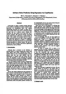
class (number of defective software modules). It is clear that the software defect prediction dataset is imbalanced in nature as the number of defective software modules is less as compared to the number of nondefective software modules. A brief description of twenty-one common basic software metrics selected from forty metrics of eight defect prediction datasets such as lines of code, cyclomatic complexity, volume, difficulty, number of operators, and operands is also provided in Table 2. More detailed description of other metrics or information about the NASA datasets can be obtained from [63]. Performance evaluation model of proposed software defect prediction system is shown in Figure 1. True Prediction (True Positive (TP) or True Negative (TN)) refers to the number of software modules which are correctly predicted as nondefective or defective software modules. While the False Prediction (False Positive (FP) or False Negative (FN)) indicates the number of software modules which are incorrectly recognized as defective or nondefective software modules. The performance of proposed software defect prediction model is evaluated by using geometric mean. Geometric mean (𝐺-Mean) is a performance evaluation metric proposed by Kubat and Matwin for binary class classification problem [64]. It is usually used to evaluate the performance of a classifier in imbalanced

Definition

LOC v(g) ev(g) iv(g)

Number of code lines Cyclomatic complexity Essential complexity Design complexity Number of operators and operands Volume Program length Difficulty Intelligence Effort to write code Effort estimate Time estimator

n

FN

Figure 1: Performance evaluation model.

Metrics

Derived Halstead

v l d i e b t lOCode lOComment lOBlank lOCodeAndComment uniq op

Basic Halstead

uniq opnd total op total opnd branchcount

Class

Defect

Line count Comment count Blank line count Count of code and comment lines Number of unique operators Number of unique operands Number of total operators Number of total operands Number of branch counts Describing whether a software module is defective or not

data distribution scenario. It measures the balanced performance of a software defect prediction approach. 𝐺-Mean is

Applied Computational Intelligence and Soft Computing

7

Effect of parameters on G-Mean

Effect of parameters on G-Mean

0.8

0.8

0.7 0.6 G-Mean

G-Mean

0.6 0.4

0.5 0.4 0.3

0.2

0.2 0.1 2

0 2 2

0 c2

−2 −4

−4

−2

2

0

0

c2

c1

0

−2 −4

(a) KC2

−4

−2

c1

(b) CM1

Effect of parameters on G-Mean

Effect of parameters on G-Mean

0.8

0.8 0.7 0.6 G-Mean

G-Mean

0.6 0.4

0.5 0.4 0.3

0.2

0.2 0 2

0.1 2 2

0 c2

0

−2 −4 −4

−2

c2

c1

(c) KC1

2

0

0

−2 −4

−4

−2

c1

(d) PC4

Figure 2: The influence of penalty parameters on 𝐺-Mean of WLSTSVM.

calculated by taking the geometric mean of sensitivity and specificity as follows: Geometric Mean = √Sensitivity × Specificity.

(25)

Sensitivity or recall and specificity are defined as Sensitivity =

TP , TP + FP

TN Specificity = . TN + FN

(26)

We have also compared the performance of the proposed software defect predictor using precision and 𝐹-measure which are defined as Precision =

TP , TP + FN

2 ∗ Precision ∗ Recall . 𝐹-measure = Precision + Recall

(27)

4.2. Parameters Selection. The proposed WLSTSVM classifier used for software prediction has two penalty parameters 𝑐1 and 𝑐2 . In this research work, we have analyzed the influence of penalty parameters on the performance of proposed system which are used in problem (13) and (16). The performance of a classifier gets affected by the selections of these parameters. This study has used Grid Search approach for the optimal parameters selection. The penalty parameters are selected from the following range: 𝑐1 , 𝑐2 ∈ {10−4 , . . . , 102 }. Figure 2 shows the influence of these parameters on the 𝐺Mean of proposed software defect prediction system for KC1, KC2, CM1, and PC4 datasets. From the figure, it is clear that the proposed system shows better performance on high value of 𝑐1 and 𝑐2 parameters (𝑐1 = 1, 𝑐2 = 1, 77.78%) for KC2 dataset. For CM1 dataset, the proposed system achieves the highest value of geometric mean on high value of 𝑐1 and low value of 𝑐2 parameter (𝑐1 = 1, 𝑐2 = 0.1, 71.98%). For KC1 dataset, WLSTSVM gains the highest geometric mean with high value of 𝑐1 and 𝑐2 parameters (𝑐1 = 1, 𝑐2 = 10, 71.73%). On the other hand, for KC1 dataset, the proposed defect predictor obtains better geometric mean with low value of

8

Applied Computational Intelligence and Soft Computing Table 3: Comparison on the basis of sensitivity values on eight datasets.

Dataset CM1 KC1 PC1 PC3 PC4 MC2 KC2 KC3

SVM 0.1511 0.1986 0.6624 0.6385 0.7296 0.5208 0.6924 0.3347

CBNN 0.5904 0.6836 0.5411 0.6055 0.6572 0.7812 0.6256 0.5072

NB 0.4402 0.3088 0.3566 0.2854 0.3855 0.3462 0.5804 0.4602

RF 0.3228 0.3161 0.4182 0.2250 0.5451 0.5569 0.5613 0.4374

LR 0.2806 0.4485 0.3194 0.2737 0.4742 0.3603 0.5995 0.2813

𝑘-NN 0.3843 0.4565 0.2968 0.4198 0.4627 0.4005 0.6859 0.5938

BBN 0.4582 0.3359 0.5591 0.3172 0.5802 0.4300 0.6450 0.5742

C4.5 0.2634 0.4285 0.3904 0.3826 0.5128 0.5546 0.5832 0.4055

LSTSVM 0.7600 0.7701 0.5387 0.6563 0.7601 0.7633 0.7569 0.7700

WLSTSVM 0.7750 0.6400 0.6791 0.5938 0.7846 0.7867 0.7804 0.7500

LSTSVM 0.6612 0.6435 0.9750 0.5742 0.6641 0.4655 0.7391 0.5506

WLSTSVM 0.6684 0.8040 0.7946 0.6981 0.7180 0.5118 0.7773 0.5882

LSTSVM 0.4225 0.9538 0.9532 0.4287 0.5310 0.7504 0.9541 0.5357

WLSTSVM 0.8685 0.9475 0.9792 0.6873 0.8667 0.8824 0.9326 0.6157

Table 4: Comparison on the basis of specificity values on eight datasets. Dataset CM1 KC1 PC1 PC3 PC4 MC2 KC2 KC3

SVM 0.9603 0.9745 0.8078 0.6004 0.8027 0.7556 0.7385 0.9164

CBNN 0.7148 0.7002 0.8342 0.7282 0.8136 0.4664 0.7684 0.7429

NB 0.8286 0.9405 0.9028 0.9066 0.8750 0.9108 0.8143 0.7976

RF 0.5883 0.6224 0.6917 0.7009 0.6173 0.6702 0.6875 0.5402

LR 0.5772 0.5818 0.6132 0.5569 0.4936 0.4080 0.5934 0.4127

𝑘-NN 0.6836 0.7082 0.7773 0.5491 0.5518 0.5422 0.6702 0.6936

BBN 0.5322 0.6501 0.7804 0.5845 0.6173 0.6867 0.6224 0.5873

C4.5 0.4274 0.5301 0.6022 0.4867 0.4682 0.3288 0.5304 0.4566

Table 5: Comparison on the basis of precision values on eight datasets. Dataset CM1 KC1 PC1 PC3 PC4 MC2 KC2 KC3

SVM 0.2562 0.4468 0.5538 0.6027 0.5166 0.5632 0.5883 0.4054

CBNN 0.3854 0.5203 0.4953 0.6228 0.6512 0.7775 0.8674 0.6484

NB 0.4038 0.4797 0.4861 0.4176 0.5648 0.6185 0.5766 0.5237

RF 0.3589 0.4282 0.4566 0.3805 0.6250 0.6393 0.6488 0.5466

LR 0.3464 0.5402 0.3536 0.4205 0.5466 0.4839 0.7063 0.5321

𝑐1 and 𝑐2 parameters (𝑐1 = 0.0001, 𝑐2 = 0.01, 75.05%). It is observed that the impact of these parameters on the 𝐺-Mean is different for each dataset and the proper choice of these parameters can improve the performance of the software defect prediction system to a great extent. Therefore, there is a need of proper combination of these parameters for other datasets also so that the software defect prediction system could achieve better predictive performance. 4.3. Result Comparison and Discussion. The performance of the proposed software defect predictor is compared with the existing approaches, including Support Vector Machine (SVM), Cost-Sensitive Neural Network (CBNN), weighted Naive Bayes (NB), Random Forests (RF), Logistic Regression (LR), 𝑘-Nearest Neighbor (𝑘-NN), Bayesian Belief Network (BBN), C4.5 Decision Tree, and Least Squares Twin Support Vector Machine (LSTSVM). All these approaches are implemented in MATLAB R2012a on Windows 7 system with Intel Core i-7 processor (3.4 GHz) with 12-GB RAM. The experiment is performed by using 10-fold cross validation

𝑘-NN 0.4200 0.6436 0.4593 0.3051 0.5501 0.4499 0.6207 0.5293

BBN 0.5203 0.4953 0.6516 0.5164 0.5278 0.5047 0.7212 0.6653

C4.5 0.3420 0.2975 0.4321 0.5163 0.4833 0.5384 0.6224 0.2991

method in which each dataset is randomly divided into ten equal sized subsets. Each time nine subsets are used as the training dataset for the learning and remaining one subset is used as the testing data for the evaluation of defect prediction system. This process is then repeated ten times so that each of the ten subsets is used exactly once as the training and testing data. The final performance of the defect prediction system is estimated by averaging of the results of 10-fold. Tables 3– 7 show the performance comparison in terms of sensitivity, specificity, precision, 𝐹-measure, and geometric mean (𝐺Mean) metrics of our proposed approach with other existing approaches on 8 software defect prediction datasets. The results include the mean of sensitivity, specificity, precision, 𝐹-measure, and geometric mean of the 10-fold. In Tables 3–7, we have mentioned the best performance of each approach. Bold figures indicate better predictive performance of a classifier for each dataset. From Table 3, it is clear that the proposed WLSTSVM based software defect predictor obtains highest sensitivity for CM1, PC1, PC4, MC2, and KC2 datasets. WLSTSVM gains the highest precision value

Applied Computational Intelligence and Soft Computing

9

Table 6: Comparison on the basis of 𝐹-measure values on eight datasets. Dataset CM1 KC1 PC1 PC3 PC4 MC2 KC2 KC3

SVM 0.1900 0.2749 0.6033 0.6200 0.6048 0.5411 0.6362 0.3667

CBNN 0.4664 0.5908 0.5172 0.6140 0.6542 0.7793 0.7269 0.5692

NB 0.4212 0.3757 0.4114 0.3391 0.4582 0.4439 0.5285 0.4899

RF 0.3398 0.3637 0.4365 0.2828 0.5823 0.5952 0.6018 0.4859

LR 0.3100 0.4900 0.3356 0.3315 0.5078 0.4130 0.6485 0.3680

𝑘-NN 0.4014 0.5341 0.3606 0.3534 0.5026 0.4237 0.6516 0.5597

BBN 0.4873 0.4003 0.6018 0.3929 0.5527 0.4643 0.6809 0.6164

C4.5 0.2975 0.3512 0.4102 0.4395 0.4976 0.5464 0.6022 0.3443

LSTSVM 0.5430 0.8522 0.6884 0.5186 0.6252 0.7568 0.8441 0.6318

WLSTSVM 0.8191 0.7639 0.8019 0.6371 0.8236 0.8318 0.8478 0.6762

LSTSVM 0.7088 0.7039 0.7247 0.6138 0.7104 0.5960 0.7479 0.6511

WLSTSVM 0.7198 0.7173 0.7345 0.6438 0.7505 0.6345 0.7788 0.6642

Table 7: Comparison on the basis of geometric mean values on eight datasets. Dataset CM1 KC1 PC1 PC3 PC4 MC2 KC2 KC3

SVM 0.3809 0.4399 0.7314 0.6191 0.7652 0.6273 0.7150 0.5538

CBNN 0.6496 0.6918 0.6718 0.6640 0.7312 0.6036 0.6993 0.6138

NB 0.6039 0.5389 0.5673 0.5086 0.5807 0.5615 0.6874 0.6058

RF 0.4358 0.4436 0.5378 0.3971 0.580 0.6109 0.6212 0.4860

LR 0.4024 0.5108 0.4425 0.3904 0.4838 0.3834 0.5964 0.3407

with CM1, PC1, PC3, PC4, and MC2 datasets. The proposed defect predictor achieves the highest 𝐹-measure for 7 out of 8 datasets as shown in Table 6. From the experimental results, it is observed that the proposed software defect predictor obtains better 𝐺-Mean on CM1, KC1, PC1, MC2, KC2, and KC3 software defect prediction datasets. Cost-Sensitive Boosting Neural Network gains the highest 𝐺-Mean for PC3 software defect prediction dataset while Support Vector Machine shows better 𝐺-Mean for PC4 defect prediction dataset. Therefore, we can conclude that WLSTSVM is an effective software predictor which is ensured by the fact that its performance is better than those of other four methods on 6 of 8 datasets in each case. 4.4. Statistical Comparison of Software Defect Predictors. The findings of experimental results are supported by Wilcoxon singed rank which is a nonparametric statistical hypothesis approach. Wilcoxon signed rank test performs pairwise comparison of two approaches used for software defect prediction and analyzes the differences between their performances on each dataset [65–67]. The rank is assigned to the differences according to their absolute values from the smallest to the largest and average ranks which are given in the case of ties. Wilcoxon signed rank stores the sum of rank in 𝑅+ and 𝑅− where 𝑅+ stores the sum of ranks for the datasets on which WLSTSVM classifier has shown better performance over other classifiers and 𝑅− stores the sum of ranks for the opposite. It determines whether a hypothesis of software defect predictors comparison could be rejected at a specified significance level 𝛼. The 𝑝 value is also computed for each comparison which shows the lowest level of significance of a hypothesis that results in a rejection. In this manner, it can be determined whether two software defect predictors are

𝑘-NN 0.5125 0.5685 0.4803 0.4801 0.5052 0.4659 0.6780 0.6417

BBN 0.4938 0.4672 0.6605 0.4305 0.5984 0.5433 0.6335 0.5807

C4.5 0.3355 0.4766 0.4848 0.4315 0.4899 0.4270 0.5562 0.4302

Table 8: Result of Wilcoxon signed rank test. Wilcoxon signed rank test Software defect predictors

𝑅+

𝑅−

𝑝 value

WLSTSVM versus SVM

33

3

0.035

WLSTSVM versus CBNN

34

2

0.025

WLSTSVM versus NB

36

0

0.011

WLSTSVM versus RF

36

0

0.011

WLSTSVM versus LR

36

0

0.011

WLSTSVM versus 𝑘-NN

36

0

0.011

WLSTSVM versus BBN

36

0

0.011

WLSTSVM versus C4.5

36

0

0.011

WLSTSVM versus LSTSVM

36

0

0.011

significantly different or the same. If different, it also determines how different they are. In order to conduct Wilcoxon signed rank test, we have performed pairwise comparison of software defect predictors in which the performance of WLSTSVM is compared with every other approach. Ranks and 𝑝 value are calculated for each case. The statistical inferences are made from the observed difference in the geometric mean as it evaluates the balanced performance of a classifier in imbalance learning scenario. The results obtained from Wilcoxon signed rank test is shown in Table 8. It is observed from the table that the 𝑝 value is less than 0.05 in all the cases; that is, the proposed software defect predictor outperforms all of them with high degree of confidence in each case.

10

5. Conclusion Class imbalance problem often occurs in software engineering and other real world applications which deteriorates the performance of machine learning approaches as they consider the equal distribution of data samples among classes and assume that the misclassification cost of each class is equally important. It is essential to incorporate the misclassification costs into the software defect prediction models as the misclassification of defective software modules incurs much higher cost than the misclassification of nondefective one. So, in this study, we have developed a software defect prediction system by using Weighted Least Squares Twin Support Vector Machine (WLSTSVM). In this approach misclassification cost is assigned to the software modules of each class in order to compensate the negative effect of the imbalanced data on the performance of software defect prediction. The performance of proposed WLSTSVM classifier is compared with nine algorithms on eight software defect prediction datasets. Experimental results demonstrate the effectiveness of our approach for the software defect prediction task. This study also performs statistical analysis of the performance of each classifier by using Wilcoxon signed rank test. The test shows that the differences between WLSTSVM and the compared approaches are statistically significant. Parameters selection is an important issue which needs to be addressed in future as they affect the prediction results to a certain extent. Selection of relevant features is another issue of concern which should be performed to improve the performance of software defect prediction system.

Conflict of Interests The authors declare that they have no conflict of interests regarding the publication of this paper.

References [1] N. Fenton and J. Bieman, Software Metrics: A Rigorous and Practical Approach, CRC Press, Boca Raton, Fla, USA, 2014. [2] N. E. Fenton and M. Neil, “Software metrics: roadmap,” in Proceedings of the Conference on the Future of Software Engineering (ICSE ’00), pp. 357–370, ACM, Limerick, Ireland, June 2000. [3] A. G. Koru and H. Liu, “Building effective defect-prediction models in practice,” IEEE Software, vol. 22, no. 6, pp. 23–29, 2005. [4] C. Catal and B. Diri, “A systematic review of software fault prediction studies,” Expert Systems with Applications, vol. 36, no. 4, pp. 7346–7354, 2009. [5] T. Hall, S. Beecham, D. Bowes, D. Gray, and S. Counsell, “A systematic literature review on fault prediction performance in software engineering,” IEEE Transactions on Software Engineering, vol. 38, no. 6, pp. 1276–1304, 2012. [6] E. Arisholm, L. C. Briand, and E. B. Johannessen, “A systematic and comprehensive investigation of methods to build and evaluate fault prediction models,” Journal of Systems and Software, vol. 83, no. 1, pp. 2–17, 2010. [7] S. Wang and X. Yao, “Using class imbalance learning for software defect prediction,” IEEE Transactions on Reliability, vol. 62, no. 2, pp. 434–443, 2013.

Applied Computational Intelligence and Soft Computing [8] J. Zheng, “Cost-sensitive boosting neural networks for software defect prediction,” Expert Systems with Applications, vol. 37, no. 6, pp. 4537–4543, 2010. [9] Y. Kamei, A. Monden, S. Matsumoto, T. Kakimoto, and K.-I. Matsumoto, “The effects of over and under sampling on faultprone module detection,” in Proceedings of the 1st International Symposium on Empirical Software Engineering and Measurement (ESEM ’07), pp. 196–204, Madrid, Spain, September 2007. [10] T. M. Khoshgoftaar, K. Gao, and N. Seliya, “Attribute selection and imbalanced data: problems in software defect prediction,” in Proceedings of the 22nd IEEE International Conference on Tools with Artificial Intelligence (ICTAI ’10), pp. 137–144, IEEE, Arras, France, October 2010. [11] J. C. Riquelme, R. Ruiz, D. Rodr´ıguez, and J. Moreno, “Finding defective modules from highly unbalanced datasets,” Actas de los Talleres de las Jornadas de Ingenier´ıa del Software y Bases de Datos, vol. 2, no. 1, pp. 67–74, 2008. [12] H. He and E. A. Garcia, “Learning from imbalanced data,” IEEE Transactions on Knowledge and Data Engineering, vol. 21, no. 9, pp. 1263–1284, 2009. [13] Jayadeva, R. Khemchandani, and S. Chandra, “Twin support vector machines for pattern classification,” IEEE Transactions on Pattern Analysis and Machine Intelligence, vol. 29, no. 5, pp. 905–910, 2007. [14] Y. Tian, Z. Qi, X. Ju, Y. Shi, and X. Liu, “Nonparallel support vector machines for pattern classification,” IEEE Transactions on Cybernetics, vol. 44, no. 7, pp. 1067–1079, 2014. [15] D. Tomar and S. Agarwal, “Twin support vector machine: a review from 2007 to 2014,” Egyptian Informatics Journal, vol. 16, no. 1, pp. 55–69, 2015. [16] O. L. Mangasarian and E. W. Wild, “Multisurface proximal support vector machine classification via generalized eigenvalues,” IEEE Transactions on Pattern Analysis and Machine Intelligence, vol. 28, no. 1, pp. 69–74, 2006. [17] M. Arun Kumar and M. Gopal, “Least squares twin support vector machines for pattern classification,” Expert Systems with Applications, vol. 36, no. 4, pp. 7535–7543, 2009. [18] Y. Sun, A. K. C. Wong, and M. S. Kamel, “Classification of imbalanced data: a review,” International Journal of Pattern Recognition and Artificial Intelligence, vol. 23, no. 4, pp. 687–719, 2009. [19] S. Kotsiantis, D. Kanellopoulos, and P. Pintelas, “Handling imbalanced datasets: a review,” GESTS International Transactions on Computer Science and Engineering, vol. 30, no. 1, pp. 25–36, 2006. [20] G. E. Batista, R. C. Prati, and M. C. Monard, “A study of the behavior of several methods for balancing machine learning training data,” ACM SIGKDD Explorations Newsletter, vol. 6, no. 1, pp. 20–29, 2004. [21] N. V. Chawla, K. W. Bowyer, L. O. Hall, and W. P. Kegelmeyer, “SMOTE: synthetic minority over-sampling technique,” Journal of Artificial Intelligence Research, vol. 16, pp. 321–357, 2002. [22] A. Estabrooks, T. Jo, and N. Japkowicz, “A multiple resampling method for learning from imbalanced data sets,” Computational Intelligence, vol. 20, no. 1, pp. 18–36, 2004. [23] Y. Liu, X. Yu, J. X. Huang, and A. An, “Combining integrated sampling with SVM ensembles for learning from imbalanced datasets,” Information Processing and Management, vol. 47, no. 4, pp. 617–631, 2011. [24] X.-Y. Liu, J. Wu, and Z.-H. Zhou, “Exploratory undersampling for class-imbalance learning,” IEEE Transactions on Systems,

Applied Computational Intelligence and Soft Computing

[25]

[26]

[27]

[28]

[29]

[30]

[31]

[32]

[33]

[34]

[35]

[36]

[37]

[38]

[39]

Man, and Cybernetics, Part B: Cybernetics, vol. 39, no. 2, pp. 539– 550, 2009. C. Bunkhumpornpat, K. Sinapiromsaran, and C. Lursinsap, “Safe-level-smote: safe-level-synthetic minority over-sampling technique for handling the class imbalanced problem,” in Advances in Knowledge Discovery and Data Mining, pp. 475– 482, Springer, Berlin, Germany, 2009. S.-J. Yen and Y.-S. Lee, “Cluster-based under-sampling approaches for imbalanced data distributions,” Expert Systems with Applications, vol. 36, no. 3, pp. 5718–5727, 2009. S. Chen, G. Guo, and L. Chen, “A new over-sampling method based on cluster ensembles,” in Proceedings of the 24th IEEE International Conference on Advanced Information Networking and Applications Workshops (WAINA ’10), pp. 599–604, IEEE, Perth, Australia, April 2010. L. Mena and J. A. Gonzalez, “Symbolic one-class learning from imbalanced datasets: application in medical diagnosis,” International Journal on Artificial Intelligence Tools, vol. 18, no. 2, pp. 273–309, 2009. B. X. Wang and N. Japkowicz, “Boosting support vector machines for imbalanced data sets,” Knowledge and Information Systems, vol. 25, no. 1, pp. 1–20, 2010. M. A. Maloof, “Learning when data sets are imbalanced and when costs are unequal and unknown,” in Proceedings of the Workshop on Learning from Imbalanced Data Sets II (ICML ’03), vol. 2, pp. 1–2, Washington, DC, USA, 2003. M. Kukar and I. Kononenko, “Cost-sensitive learning with neural networks,” in Proceedings of the 13th European Conference on Artificial Intelligence (ECAI ’98), 1998, pp. 445–449. W. Fan, S. J. Stolfo, J. Zhang, and P. K. Chan, “AdaCost: misclassification cost-sensitive boosting,” in Proceedings of the 16th International Conference on Machine Learning (ICML ’99), pp. 97–105, Bled, Slovenia, June 1999. D. Tomar and S. Agarwal, “An effective weighted multi-class least squares twin support vector machine for imbalanced data classification,” International Journal of Computational Intelligence Systems, vol. 8, no. 4, pp. 761–778, 2015. S. Kanmani, V. R. Uthariaraj, V. Sankaranarayanan, and P. Thambidurai, “Object-oriented software fault prediction using neural networks,” Information and Software Technology, vol. 49, no. 5, pp. 483–492, 2007. T. M. Khoshgoftaar, E. B. Allen, W. D. Jones, and J. P. Hudepohl, “Classification tree models of software quality over multiple releases,” in Proceedings of the 10th International Symposium on Software Reliability Engineering (ISSRE ’99), pp. 116–125, Boca Raton, Fla, USA, November 1999. R. W. Selby and A. A. Porter, “Learning from examples: generation and evaluation of decision trees for software resource analysis,” IEEE Transactions on Software Engineering, vol. 14, no. 12, pp. 1743–1757, 1988. K. O. Elish and M. O. Elish, “Predicting defect-prone software modules using support vector machines,” Journal of Systems and Software, vol. 81, no. 5, pp. 649–660, 2008. G. Czibula, Z. Marian, and I. G. Czibula, “Software defect prediction using relational association rule mining,” Information Sciences, vol. 264, pp. 260–278, 2014. L. Guo, Y. Ma, B. Cukic, and H. Singh, “Robust prediction of fault-proneness by random forests,” in Proceedings of the 15th International Symposium on Software Reliability Engineering (ISSRE ’04), pp. 417–428, Saint-Malo, France, November 2004.

11 [40] S. Agarwal, D. Tomar, and Siddhant, “Prediction of software defects using twin support vector machine,” in Proceedings of the International Conference on Information Systems and Computer Networks (ISCON ’14), pp. 128–132, IEEE, Mathura, India, March 2014. [41] V. U. B. Challagulla, F. B. Bastani, I.-L. Yen, and R. A. Paul, “Empirical assessment of machine learning based software defect prediction techniques,” International Journal on Artificial Intelligence Tools, vol. 17, no. 2, pp. 389–400, 2008. [42] J. Moeyersoms, E. Junqu´e De Fortuny, K. Dejaeger, B. Baesens, and D. Martens, “Comprehensible software fault and effort prediction: a data mining approach,” Journal of Systems and Software, vol. 100, pp. 80–90, 2015. [43] A. Okutan and O. T. Yıldız, “Software defect prediction using Bayesian networks,” Empirical Software Engineering, vol. 19, no. 1, pp. 154–181, 2014. [44] S. Amasaki, Y. Takagi, O. Mizuno, and T. Kikuno, “A Bayesian belief network for assessing the likelihood of fault content,” in Proceedings of the 14th IEEE International Symposium on Software Reliability Engineering (ISSRE ’03), pp. 215–226, IEEE, Denver, Colo, USA, November 2003. [45] S. Bibi and I. Stamelos, “Software process modeling with Bayesian belief networks,” in Proceedings of the 10th International Software Metrics Symposium (METRICS ’04), vol. 14, p. 16, Chicago, Ill, USA, September 2004. [46] K. Dejaeger, T. Verbraken, and B. Baesens, “Toward comprehensible software fault prediction models using bayesian network classifiers,” IEEE Transactions on Software Engineering, vol. 39, no. 2, pp. 237–257, 2013. [47] G. J. Pai and J. B. Dugan, “Empirical analysis of software fault content and fault proneness using Bayesian methods,” IEEE Transactions on Software Engineering, vol. 33, no. 10, pp. 675– 686, 2007. [48] N. Fenton, M. Neil, and D. Marquez, “Using Bayesian networks to predict software defects and reliability,” Proceedings of the Institution of Mechanical Engineers, Part O, vol. 222, no. 4, pp. 701–712, 2008. [49] C. Catal and B. Diri, “Investigating the effect of dataset size, metrics sets, and feature selection techniques on software fault prediction problem,” Information Sciences, vol. 179, no. 8, pp. 1040–1058, 2009. [50] M. Evett, T. Khoshgoftar, P. D. Chien, and E. Allen, “GP-based software quality prediction,” in Proceedings of the 3rd Annual Genetic Programming Conference (GP ’98), pp. 60–65, Madison, Wis, USA, July 1998. [51] A. B. de Carvalho, A. Pozo, and S. R. Vergilio, “A symbolic faultprediction model based on multiobjective particle swarm optimization,” Journal of Systems and Software, vol. 83, no. 5, pp. 868–882, 2010. [52] O. Vandecruys, D. Martens, B. Baesens, C. Mues, M. De Backer, and R. Haesen, “Mining software repositories for comprehensible software fault prediction models,” Journal of Systems and Software, vol. 81, no. 5, pp. 823–839, 2008. ¨ F. Arar and K. Ayan, “Software defect prediction using cost[53] O. sensitive neural network,” Applied Soft Computing, vol. 33, pp. 263–277, 2015. [54] T. M. Khoshgoftaar and K. Gao, “Feature selection with imbalanced data for software defect prediction,” in Proceedings of the 8th International Conference on Machine Learning and Applications (ICMLA ’09), pp. 235–240, Miami Beach, Fla, USA, December 2009.

12 [55] X. Y. Jing, S. Ying, Z. W. Zhang, S. S. Wu, and J. Liu, “Dictionary learning based software defect prediction,” in Proceedings of the 36th International Conference, pp. 414–423, ACM, Hyderabad, India, May 2014. [56] S. Agarwal and D. Tomar, “A feature selection based model for software defect prediction,” International Journal of Advanced Science and Technology, vol. 65, pp. 39–58, 2014. [57] J. C. Munson and T. M. Khoshgoftaar, “The detection of faultprone programs,” IEEE Transactions on Software Engineering, vol. 18, no. 5, pp. 423–433, 1992. [58] S. S. Rathore and A. Gupta, “A comparative study of featureranking and feature-subset selection techniques for improved fault prediction,” in Proceedings of the 7th India Software Engineering Conference (ISEC ’14), p. 7, ACM, Chennai, India, February 2014. [59] I. Chawla and S. K. Singh, “An automated approach for bug categorization using fuzzy logic,” in Proceedings of the the 8th India Software Engineering Conference, pp. 90–99, ACM, Bangalore, India, Feburary 2015. [60] K. Muthukumaran, A. Rallapalli, and N. L. Murthy, “Impact of feature selection techniques on bug prediction models,” in Proceedings of the 8th India Software Engineering Conference, pp. 120–129, ACM, Bangalore, India, Feburary 2015. [61] M. D’Ambros, M. Lanza, and R. Robbes, “An extensive comparison of bug prediction approaches,” in Proceedings of the 7th IEEE Working Conference on Mining Software Repositories (MSR ’10), pp. 31–41, Cape Town, South Africa, May 2010. [62] E. Erturk and E. A. Sezer, “A comparison of some soft computing methods for software fault prediction,” Expert Systems with Applications, vol. 42, no. 4, pp. 1872–1879, 2015. [63] Software Defect Dataset, Promise Repository, May 2015, http:// promise.site.uottawa.ca/SERepository/datasets-page.html. [64] M. Kubat and S. Matwin, “Addressing the curse of imbalanced training sets: one-sided selection,” in Proceedings of the 14th International Conference on Machine Learning (ICML ’97), vol. 97, pp. 179–186, Banff, Canada, 1997. [65] A. Fern´andez, V. L´opez, M. Galar, M. J. Del Jesus, and F. Herrera, “Analysing the classification of imbalanced data-sets with multiple classes: binarization techniques and ad-hoc approaches,” Knowledge-Based Systems, vol. 42, pp. 97–110, 2013. [66] J. Demˇsar, “Statistical comparisons of classifiers over multiple data sets,” The Journal of Machine Learning Research, vol. 7, pp. 1–30, 2006. [67] D. Sheskin, Handbook of Parametric and Nonparametric Statistical Procedures, Chapman & Hall/CRC, 2nd edition, 2006.

Applied Computational Intelligence and Soft Computing

Journal of

Advances in

Industrial Engineering

Multimedia

Hindawi Publishing Corporation http://www.hindawi.com

The Scientific World Journal Volume 2014

Hindawi Publishing Corporation http://www.hindawi.com

Volume 2014

Applied Computational Intelligence and Soft Computing

International Journal of

Distributed Sensor Networks Hindawi Publishing Corporation http://www.hindawi.com

Volume 2014

Hindawi Publishing Corporation http://www.hindawi.com

Volume 2014

Hindawi Publishing Corporation http://www.hindawi.com

Volume 2014

Advances in

Fuzzy Systems Modelling & Simulation in Engineering Hindawi Publishing Corporation http://www.hindawi.com

Hindawi Publishing Corporation http://www.hindawi.com

Volume 2014

Volume 2014

Submit your manuscripts at http://www.hindawi.com

Journal of

Computer Networks and Communications

 Advances in 

Artificial Intelligence Hindawi Publishing Corporation http://www.hindawi.com

Hindawi Publishing Corporation http://www.hindawi.com

Volume 2014

International Journal of

Biomedical Imaging

Volume 2014

Advances in

Artificial Neural Systems

International Journal of

Computer Engineering

Computer Games Technology

Hindawi Publishing Corporation http://www.hindawi.com

Hindawi Publishing Corporation http://www.hindawi.com

Advances in

Volume 2014

Advances in

Software Engineering Volume 2014

Hindawi Publishing Corporation http://www.hindawi.com

Volume 2014

Hindawi Publishing Corporation http://www.hindawi.com

Volume 2014

Hindawi Publishing Corporation http://www.hindawi.com

Volume 2014

International Journal of

Reconfigurable Computing

Robotics Hindawi Publishing Corporation http://www.hindawi.com

Computational Intelligence and Neuroscience

Advances in

Human-Computer Interaction

Journal of

Volume 2014

Hindawi Publishing Corporation http://www.hindawi.com

Volume 2014

Hindawi Publishing Corporation http://www.hindawi.com

Journal of

Electrical and Computer Engineering Volume 2014

Hindawi Publishing Corporation http://www.hindawi.com

Volume 2014

Hindawi Publishing Corporation http://www.hindawi.com

Volume 2014