Prediction of Friction Stir Welding Characteristic Using Neural Network

JJMIE

Volume 2, Number 3,Sep. 2008 ISSN 1995-6665 Pages 151 - 155

Jordan Journal of Mechanical and Industrial Engineering

Prediction of Friction Stir Welding Characteristic Using Neural Network Y. K. Yousif a *, K. M. Daws b, B. I. Kazem b a

Department of Mechatronics Engineering, Baghdad University, Baghdad, Iraq Department of Mechanical Engineering, Baghdad University, Baghdad, Iraq

b

Abstract An artificial neural network (ANN) model was developed for the analysis and simulation of the correlation between the friction stir welding (FSW) parameters of aluminum (Al) plates and mechanical properties. The input parameters of the model consist of weld speed (Ws) and tool rotation speed (Rs). The outputs of the ANN model include property parameters namely: tensile strength, yield strength and elongation. Good performance of the ANN model was achieved. The model can be used to calculate mechanical properties of welded Al plates as functions of weld speed and Rs. The combined influence of weld speed and Rs on the mechanical properties of welded Al plates was simulated. Simulated annealing technique was used to prevent the network from getting stuck in local minima. A comparison was made between measured and calculated data. The calculated results were in good agreement with measured data. © 2008 Jordan Journal of Mechanical and Industrial Engineering. All rights reserved

Keywords: Friction stir welding; Mechanical properties; ANN; Modeling;

1. Introduction Recently, because of aluminum’s light weight, it has been considered an energy-saving structural material in advanced applications. In addition, aluminum is an easily saved resource because it can be recycled, and thus can be expected to be an environmental friendly metallic material. One such application would be use in automobiles, which would facilitate transportation; numerous similar examples could be cited in support of employing aluminum as a structural material. Friction stir welding (FSW) was developed initially for aluminum alloys, by the welding institute (TWI) of United Kingdom [1]. Friction stir welding (FSW) is a relatively new method invented by The Welding Institute (TWI) in 1991. FSW is actually a solid-state joining process that is a combination of extruding and forging and is not a true welding process. Since the process occurs at a temperature below the melting point of the work piece material, FSW has several advantages over fusion welding. Some of the process advantages are given in the following list [2]: 1. FSW is energy efficient 2. FSW requires minimal, if any, consumables. 3. FSW produces desirable microstructures in the weld and heat-affected zones

* Corresponding author. e-mail: [email protected]

4. FSW is environmentally "friendly" (no fumes, noise, or sparks) 5. FSW can successfully join materials that are "unweldable" by fusion welding methods. 6. FSW produces less distortion than fusion welding techniques.

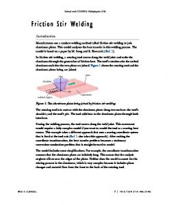
Figure (1) Schematic diagram of the FSW process

There are many research related to an applications of Artificial Intelligence (AI), especially Artificial Neural Networks (ANN) for engineering fields such as manufacturing processes prediction, monitoring and controlling. A. Bezazi , S. Gareth et al. (2006) [3]. An ANN model was developed to estimate fatigue lifetime of a sandwich composite material structure subjected to cyclic three-point bending loads. A total of 27 samples (three different loading levels for nine samples each) were

152

© 2008 Jordan Journal of Mechanical and Industrial Engineering. All rights reserved - Volume 2, Number 3 (ISSN 1995-6665)

investigated to provide training and testing data for a series of multi-layer perceptron ANNs. P. Dutta and D. K. Pratihar (2007) [4]. Conventional regression analysis was carried out on some experimental data of a tungsten inert gas (TIG) welding process , to find its input output relationships. One thousand training data for NNs were created at random, by varying the input variables within their respective ranges and the responses were calculated for each combination of input variables by using the response equations obtained through the above conventional regression analysis. Friction stir welding uses a cylindrical, shouldered tool with a profiled pin that is rotated and slowly plunged into the joint line between two pieces of sheet or plate material, which are butted together. Frictional heat is generated between the wear resistant welding tool and the work piece. This heat causes the work piece material to soften without reaching the melting point and allows the tool to traverse the weld line. As it does, the plasticized material is transferred from the leading edge of the tool to the trailing edge of the tool shoulder and pin. It leaves a solid phase bond between the two work pieces as shown in figure 1. [5] In the field of biology, electronics, computer science mathematics and engineering, ANN is one of the most important research areas. ANN is a complicated system composed of numerous nerve cells. It is also a new type of computer system which is based on the primary understanding of the organization, structure, function and mechanism of the human brain. With the help of rapid progress in computers and material science, material design can now be carried out based on the knowledge and experience of the fabricated materials [6–7].

Plunged depth of the rotating tool was 2 mm. A schematic representation of the welding instrument is given in Fig. 1. Welding was carried out by rotating the tool at 710, 900 and 1400 rpm and by moving the plates at 70,40 and 140 mm/min. By using the predetermined welding parameters, different samples were welded for mechanical tests and metallographic examinations. For the tensile tests, FSW specimens were cut by using a slow speed diamond wheel saw through the transverse direction of the bonding interface of 5, 25, 72 mm3. Tensile strength and bending stress were measured to check the mechanical performance of the welding (Table 2). measured to check the mechanical performance of the welding (Table 2). Welded samples were characterized by means of tensile strength, hardness and elongation.. It is known that increasing the welding speed and decreasing the rotational speed of the tool reduces the heat input. Thus, increase in welding speed also increases the tensile strength while increasing Rs decreases the tensile strength. Tensile test gives an information about the elongation of the FSW samples. Here, again the amount of heat input plays an important role on the elongation properties of the FSW samples. The more heat input is the more elongation of the FSW samples. The sample welded with the 1400 rpm of the tool and 70 mm/min showed the largest elongation while the sample welded with the 710 rpm of the tool and 70 mm/min yielded the minimum elongation. Welding with the fastest speed and slowest rotational speed gave a planar bonding surface while welding with lowest welding speed and fastest rotational speed of the tool gave well distinguished undulated joining edges of the plates.

2. Experimental Work

3. Methodology of ANN Application and Modeling Data with Network

Table 1 : The chemical composition of aluminum alloy Element

Percentage

Element

Percentage 0.35%

Al

-

Si

Zn

4.2%

Cu

0.2%

Mg

1.26%

Zr

0.05%

Mn

0.09%

Ti

0.05%

Fe

0.22%

Cr

0.05%

The chemical composition of the material was given in table 1. Two hot rolled aluminum plates were clamped with a vice so that they would not be separated during welding process. A rotating tool which has a diameter of 20 mm was used.

Since most manufacturing processes are complex in nature, highly non- linear and there are a large number of input variables, there is no close mathematical model which can describe the behavior of these processes. Artificial neural networks because they are cost - effective, easy to understand and because of their ability to learn from examples, have found many applications in process modeling for monitoring and control purposes, as intelligent sensors, to estimate variable that usually cannot be measured on - line, in dynamic system identification, in fault detection and diagnosis and, finally, in process control [8].

Table (2) Measured data used as data sets set No. 1 2 3 4 5 6 8 9 10

σt

NN Response

σb

NN Response

Elo. %

NN Response

78 248 281.88 336.96 320 320 297.61 189.48 246.25

77.973054 248.010246 281.865578 336.936103 319.96774 320.011411 297.614452 189.480733 246.250232

290.04 454.64 322.77 583.61 322.7 502.44 345.4 394.73 308.38

289.946098 454.633699 322.527211 583.331025 322.630815 502.380949 345.537933 394.725282 308.371768

2.4 5.64 9.2 22 11.6 11.6 15.85 4.34 11.07

2.3912949 5.6404608 9.1897045 21.987097 11.59386 11.598177 15.850173 4.3399821 11.06998

153

© 2008 Jordan Journal of Mechanical and Industrial Engineering. All rights reserved - Volume 2, Number 3 (ISSN 1995-6665)

4. Neural Network Simulation Testing of neural network model required new independent (test sets) to validate the generalization capability of network. Table (3) shows testing data sets for the network and the response of the network to these data sets. The prediction accuracy for the testing patterns based on mean absolute percent error (APE) criteria [10]:

Predicted - Actual

APE =

Actual

*100%

Ts Rs Bs Ws Elo

i j Inputs Layers

Hidden Layers

z

k

Outputs Layer

Fig (2) neural network architecture for FSW Table (3) Test data sets and network response Set σt No. 3 330 7

320

NN Response 327.125

389.8

NN Response 373.634

328.427

450.2

402.442

σb

8

NN Response 6.87832

11.6

10.4471

Elo. %

The corresponding table above the mean error of: • The Error of the Tensile Stress 1.7524 %. • The Error of the Bending Stress 7.3777 %. • The Error of the Elongation 11.98 %. 450 Bending MPa

400 350 Test Set 3

300

Tensile MPa

250 200 150 100 Actual

50

Elongation %

Pridicted

0 1

1.2 1.4 1.6 1.8

2 2.2 2.4 2.6 2.8 Pattern

3

Figure (3) Predicted and measured data in test set 3

500 Bending MPa

450 400 350 Test Set 7

ANNs are computational models, which replicate the function of a biological network, composed of neurons and are used to solve complex functions in various applications. The system has four layers, which are input, two hidden and output layers. The input layer consists of all the input factors. Information from the input layer is then processed in the course of two hidden layers, following output vector is computed in the final (output) layer. Neural networks consist of simple synchronous processing elements that are inspired by the biological nerve systems. The basic unit in the ANN is the neuron. Neurons are connected to each other by links known as synapses; associated with each synapse there is a weight factor. Details on the neural network modeling approach are given in elsewhere [9,10]. In this work, the neural network model was trained using two different training algorithms: 1. Gradient Descent with Momentum Algorithm. 2. Levenberg - Marquardt Algorithm. The performances of these two training algorithms are compared to decide which algorithm performs better than the other. The neural network may converge to a local minimum rather than a global one. Therefore, some sort of simulated annealing technique is used to find the best solution among many local minima [11]. The simulated annealing technique is as follows: once the network converges to a local minimum, the network state is perturbed in a random direction and by a random magnitude. Then the network dynamics are reactivated, and another local minimum is found. During this process, the algorithm keeps track of the best solution. After a predetermined number of local minima are found, the algorithm terminates and the solution with the lowest error is accepted as the best solution. The simulated annealing technique is used to capture the best solution (weights and biases) among several local minima. Thus, training algorithm is performed five times for each network architecture, each time with different random initial weights and biases. After examining the performance of different architectures, a network with two hidden layers (include 3 neurons in the first and 6 in the second) trained by Levenberg Marquardt algorithm showed good performance indication. while figure (2) shows the resulted network architecture. Thus, the network architecture consists of two input neurons, 9 hidden neurons with nonlinear activation function. (logarithmical sigmoid) and single output neuron with linear activation function. Tables (4,5 and 6) shows the trained network weights and biases. It is worth to note that the network training and simulation was performed on 2.8 GHZ, Pentium 4 PC using the MATLAB platform version 7 neural network toolbox.

Tensile MPa

300 250 200 150 100

Actual Pridicted

50 0 1

1.2

1.4

1.6

Elongation %

1.8

2 2.2 Pattern

2.4

2.6

Figure (4) Predicted and measured data in test set 7

2.8

3

154

© 2008 Jordan Journal of Mechanical and Industrial Engineering. All rights reserved - Volume 2, Number 3 (ISSN 1995-6665)

5. Evaluation of Results Figures (3) and (4) show the measured and predicted output values were close to each other. In all the cases of the present work, feed-forward artificial neural networks were used. In present work, the following steps were developed: 1. Database collection. 2. Analysis and pre-processing of the data. 3. Training of the neural network. 4. Test of the trained network. 5. Postprocessing of data. 6. Use of the trained NN for simulation and prediction. It's sufficient to take Rs and the welding speed to predict the mechanical properties such as tensile strength, bending stress and elongation of the bonded Al metal. In present study, Rs and the welding speed were used in the input layer and the tensile strength, bending stress and elongation were used in output. The transfer function log sigmoid used in this study is given by:

Yi =

Table (4) Weights and bias between input layer and first hidden layer 1

2

j

w1

w2

b1

1

-4.133123671

-5.808140227

2.940544626

2

16.46260301

-11.33170622

-3.74267169

3

-6.151224848

7.846399395

0.18585865

p(1)

p(1)

a(1)

a(1)

Layer 1

a(2)

Layer 2

a(2)

a(3)

y(1)

1

2

3

k

w3

w4

w5

b2

1

-14.735

5.86886

-4.4835

3.28278

2

-5.5828

-7.8937

-2.8578

8.20656

3

-5.5647

-16.739

-9.4099

12.5084

4

0.50508

-0.6692

-12.961

4.71296

5

-0.4468

8.57969

-14.071

2.45288

6

-4.7725

8.02553

3.35714

-5.4787

Weight

p

LW(1,1) bias b(1)

bias

+ +

Mz

netsum

Nz purelin

1 Y

b(3) layer simulation Figure (7) Output

G k = w k 3 * F1 + w k 4 * F2 + w k 5 * F3 + b k 1 where k = 1,2,3,4,5,6 1 Hk = - G +G +G +G +G +G 1+ e ( 1 2 3 4 5 6 ) Table (6) Weights and bias between second hidden layer and outputs Weights Bias k 1 2 3 4 5 6 b3 z 1 -1.9641 0.0739 0.6339 -5.9474 6.18 1.694 0.2263 2

4.04

-9.5196 7.3865 -13.046 9.1743 -5.8381

3.78

Ej

+ + netsum

Fj

‫ﮑ‬

logsig

Weight LW(2,1) bias b(2)

Figure (6) Two hidden layers simulation

Gk

+ + netsum1

‫ﮑ‬

result

of

network

(mechanical

Tensile strength = H 1 *w 11 + H 2 *w 12 + H 3 *w 13 + H 4 *w 14 + H 5 *w 15 + H 6 *w 16 + b13 Bending Stress =

H 1 *w 21 + H 2 *w 22 + H 3 *w 23 + H 4 *w 24 + H 5 *w 25 + H 6 *w 26 + b 23 Elongation % = H 1 *w 31 + H 2 *w 32 + H 3 *w 33 + H 4 *w 34 + H 5 *w 35 + H 6 *w 36 + b33

1

Layer 3

Table (5) Weights and bias between first and second in hidden layer

1

LW(3,2)

And must transform the result value to real value by Post processing.

Figure (5) Three layers of neural network (predictor model)

j

Weight

a(2)

Then the final properties) are:

Where Xi is the input of the neuron in hidden layer and Yi is the output of neuron while calculating Xi, Rs and Ws values must be normalize in rang [-1, 1] corresponding to the minimum and maximum of the actual values.

1

Hk

3 -2.3636 -5.8093 4.8388 -7.7474 6.2868 2.4715 1.5288

1 1 + e -X i

i

1

Hk

logsig1

1 a(2)

6. Conclusion

The aim of this paper was to show the possibility of the use of neural networks for the calculation of the mechanical properties of welded Al plates using FSW method. Results showed that, the networks can be used as an alternative way in these systems. For the proposed NN model the Levenberg – Marquardt algorithm shows better performance than gradient descent with momentum because it use 2nd order Taylor series approximation of performance index rather than 1St order approximation as with gradient descent algorithm. It is found that the correlations between the measured and predicted values of tensile strength, bending stress were better than those of elongation.

© 2008 Jordan Journal of Mechanical and Industrial Engineering. All rights reserved - Volume 2, Number 3 (ISSN 1995-6665)

References [1] Tomotake Hirata et al."Influence of friction stir welding parameters on grain size and formability in 5083 aluminum alloy" Graduate School of Engineering, Osaka Prefecture University, 2006. [2] Nicholas, ED, "Developments in the friction stir welding of metals". ICAA-6: 6th International Conference on Aluminum Alloys, Japan, 1998. [3] Bezazi , S. Gareth et al." Fatigue life prediction of sandwich composite materials under flexural tests using a Bayesian trained artificial neural network" International Journal of Fatigue, Vol. 29, 2007, 738–747. [4] P. Dutta and D. K. Pratihar " Modeling of TIG welding process using conventional regression analysis and neural network-based approaches", Journal of Materials Processing Technology, Department of Mechanical Engineering, Indian Institute of Technology, Vol. 184, 2007, 56-68. [5] M. Abbasi Gharacheh, A.H. Kokabi, G.H. Daneshi, B. Shalchi, R. Sarrafi "The influence of the ratio of ‘‘rotational speed/traverse speed’’ (o/v) on Mechanical properties of AZ31 friction stir welds" International Journal of Machine Tools & Manufacture, Vol. 46, 2006,

155

[6] Zeng Qingfeng, Zu Jiakui, Zhang Litong, Dai Guanzhong Mater, Vol. 23, 2002, 287–290. [7] Marmey P, Porte´ MC, Baquey C. Nucl Instrum Meth Phys Res Sect B: Beam Interact Mater Atoms, Vol. 208, 2003, 429–433. [8] Hang and Chen," neural network based tool breakage monitoring system for end milling", Journal of Industrial Technology, Vol.16, No.2, 2000. [9] Massie DD. ECOS 2001. In: Gogus YA, Ozturk A, editors. First International Conference on Applied Thermodynamics, Istanbul, Turkey, 2001. [10] Malinov S, Sha W, McKeown JJ, "Modelling the correlation between processing parameters and properties in Titanium alloys using artificial neural network", Computational Materials Science, Vol. 21, 2001, 375-394. [11] Tania Binos "Evolving Neural Network Architecture and Weights Using An Evolutionary Algorithm" MSc Thesis, Department of Computer Science, RMIT University, Austalia, 2003. [12] R. Azouzi and M. Guillot "On-line optimization of the turning process using an inverse process neurocontroller", Journal of Manufacturing Science and Engineering, Vol. 120, 1998, 101-108.