Prediction of geometric errors of robot manipulators with Particle ...

Robotics and Autonomous Systems 54 (2006) 956–966 www.elsevier.com/locate/robot

Prediction of geometric errors of robot manipulators with Particle Swarm Optimisation method G¨ursel Alıcı a,∗ , Romuald Jagielski b , Y. Ahmet S¸ekercio˘glu c , Bijan Shirinzadeh d a Faculty of Engineering, University of Wollongong, Australia b Department of Electrical and Computer Systems Engineering, Monash University, Australia c Centre for Telecommunication and Information Engineering, Monash University, Australia d Department of Mechanical Engineering, Monash University, Australia

Received 24 March 2005; received in revised form 24 May 2006; accepted 16 June 2006 Available online 1 August 2006

Abstract This paper reports on the prediction of the expected positioning errors of robot manipulators due to the errors in their geometric parameters. A Swarm Intelligence (SI) based algorithm, which is known as Particle Swarm Optimization (PSO), has been used to generate error estimation functions. The experimental system used is a Motoman SK120 manipulator. The error estimation functions are based on the robot position data provided by a high precision laser measurement system. The functions have been verified for three test trajectories, which contain various configurations of the manipulator. The experimental results demonstrate that the positioning errors of robot manipulators can be effectively predicted using some constant coefficient polynomials whose coefficients are determined by employing the PSO algorithm. It must be emphasized that once the estimation functions are obtained, there may be no need of any further experimental data in order to determine the expected positioning errors for a subsequent use in the error correction process. c 2006 Elsevier B.V. All rights reserved.

Keywords: Robot calibration; Particle Swarm Optimization; Error estimation and correction

1. Introduction The accuracy of robot manipulators can be significantly improved by implementing the calibration process that consists of modeling, measurement, identification and correction stages. Of these, the identification stage provides better estimates of the parameters of the kinematic model. Even if it is possible to dismantle a robot manipulator and determine the parameters in its kinematic model, the resulting model will still contain some inaccuracies arising from joint and link compliances changing with the manipulator configurations [3], steady state errors in joint positions, inaccurate knowledge of the kinematic parameters, and payload carried by the manipulator. It follows that it is necessary to identify parameters in the kinematic model, and then consider them in kinematic error correction, especially when it is not possible to use absolute end point measurements for position feedback. As a result, ∗ Corresponding author. Fax: +61 2 4221 3101.

E-mail address: [email protected] (G. Alıcı). c 2006 Elsevier B.V. All rights reserved. 0921-8890/$ - see front matter doi:10.1016/j.robot.2006.06.002

a considerable amount of research has been devoted to the kinematic identification and calibration of robotic systems [9–11,13,17,21–26]. For example, Jang et al. [13] have presented a calibration methodology based on dividing the manipulator workspace into several local regions, and subsequently building a calibration equation using a three dimensional position measurement system consisting of a camera and infrared LED. In the work relevant to this study [16], the calibration of a Motoman P-8 robot was performed using circle point analysis technique, which requires external hardware to determine the manipulator end point positions in Cartesian space. Although the topology of their experimental system contained a five-bar mechanism, the kinematic parameters of the mechanism had not been taken into account during the kinematic calibration. Driels and Pathre [9] have reported on the effects of initial estimates of parameters, measurement accuracy and noise, encoder resolution and uncertainty, selection of measurement configurations, and of the number of measurements on

G. Alıcı et al. / Robotics and Autonomous Systems 54 (2006) 956–966

957

Table 1 The results of D–H parameters for a Motoman 120 SK manipulator and the parallel mechanism

The shaded rows are for the parallel mechanism.

Fig. 1. Schematic representation of the robot manipulator with D–H convention and parameters. Note that the coordinate frames O2 and O¯ 3 , and O4 and O5 are located at the same point.

the identification and observability of kinematic parameters through a number of simulation results. Hollerbach and Wampler [11] have provided a full account of previous work in kinematic identification and calibration of robotic systems, and introduced a calibration index based on the system mobility equation. Zak et al. [22] proposed a kinematic parameter estimation methodology, where a classical least square estimation algorithm is replaced with a weighted least square. Simulation results were presented to demonstrate that it was possible to further improve the parameter estimates without increasing the number of measurements. Renders et al. [17] presented a robot kinematic parameter identification technique based on a maximum likelihood algorithm in a recursive form with a reasonable amount of computation time. Over the last three decades, optimization methods inspired by the complex natural systems have been used successfully in a huge number of applications. Among them, artificial neural networks, granular and evolutionary computation are the most well known ones. In recent years, a new optimization method has been developed based on the observations of intelligent and efficient behavior of an overall system resulting from the cooperation of individual entities employing a set of relatively simple rules [4,6,8]. Biological examples of this method include ant colonies, fish flocks and bee swarms. In these examples, individuals communicate and coordinate via a set of relatively simple rules, and their local interaction and goal directed behavior lead to a global optimization of the overall system. Artificial intelligence methods inspired by these natural systems are called Swarm Intelligence [SI]. Successful applications of SI, especially the Particle Swarm Optimization [PSO] algorithm, to optimization problems have inspired us to employ it for predicting positioning errors of robot manipulators. PSO is a method proposed by Kennedy and Eberhart [15], and the algorithm is based on the foraging behavior of animals, especially birds.

It is virtually impossible to consider all the sources contributing to the pose errors while forming the kinematic model of a robot manipulator. We, therefore, believe that the search for yet more complex models to be incorporated within the identification model to be a fruitless task. If the pose errors of a robot manipulator are known as a function of the manipulator configuration, they can be appropriately corrected using a ‘false target’ technique [17]. With this in mind, the determination of pose errors or positioning errors only (as is the case in this study due to fact that the measurement system can provide only position data) is considered as a blackbox problem, employing computational models based on the PSO algorithm. In this study, the computational model is based on estimator functions that are generated automatically using the position data for 85 identification configurations of the manipulator measured by a high precision laser tracking system [1–3]. Experimental results demonstrate that the robot positioning errors can be effectively estimated using PSO based optimization methods. This work contributes to previously published work from the point of view of being a simple and systematic approach to the self-calibration of robotic systems with minimum experimental data. 2. Kinematic model The schematic of the robot manipulator and the coordinate frames needed to generate a kinematic model based on Denavit–Hartenberg parameters are depicted in Fig. 1. The kinematic model for the parallel five-bar mechanism is also included in the overall model. The Denavit–Hartenberg parameters for the manipulator and the parallel mechanism are given in Table 1. An L-shaped apparatus with a longitudinal extension of 112.65 mm from the manipulator tool plate and a vertical offset of 205.32 mm from the longitudinal axis of the tool plate is connected to the manipulator tool plate in order to secure the retroreflector of the measurement system to the robot via a 3-point-contact magnetic fixture. This makes D6 = 342.65 mm, and D6 = 205.32 mm. With reference to Fig. 1, it must be noted that, for the five-bar mechanism, θ¯1 = θ3 , θ¯2 = θ2 − θ3 , θ¯2 + θ¯3 = π, L¯ 1 = L¯ 3 and L¯ 2 = L 2 . The homogeneous transformation matrix between frames 1 and 2 of the five-bar mechanism is described by, 1

¯

¯

T 2 = (1 T 1¯ )(1 T 2¯ )(2 T 3¯ ).

(1)

958

G. Alıcı et al. / Robotics and Autonomous Systems 54 (2006) 956–966

The overall transformation matrix between the base coordinate frame and the frame fixed to the manipulator end point is written as 0

¯

T 6 = (0 T 1 )(1 T 2 )(3 T 3 )(3 T 4 )(4 T 5 )(5 T 6 )

(2)

where j T j + 1 is the homogeneous transformation matrix between two consecutive coordinate frames j and j + 1 based on the Denavit–Hartenberg convention [18]. 3. Models of position errors It has been reported in the literature that the gear train errors [21], the errors due to structural deformations [10], and the errors due to the geometric parameters of the model [13] can be represented by a cyclic function of the joint angles. Based on this, we assume that the positioning errors change with the joint positions, i.e., 1p = f (θi ). Another assumption we make is that the locus of the positioning errors for selected identification configurations is a piecewise continuous random function. It follows that the loci of the Cartesian errors of robot manipulators while following a given trajectory are in the form of bounded and integrable/summable functions. With reference to the Theorem of Weierstrass [12,19] for approximating continuous or discontinuous functions with polynomials, if a given function of p(θ ) is continuous or piecewise continuous, bounded and integrable within an interval of a ≤ θ ≤ b and ε is an arbitrary positive quantity indicating the convergence tolerance, p(θ ) can be approximated with a polynomial F(θ ) within the defined interval such that | p(θ) − F(θ )| < ε.

(3)

F(θ) can be of any type of polynomials including Fourier polynomials, ordinary polynomials, and other well-known polynomials of Jacobi, Laguerre and Hermite, and Bessel. In this study, Fourier and ordinary polynomials are considered for position error approximation. It had been demonstrated a long time ago [13] that if p(θ ) has a discontinuity at θ = θ0 , the polynomial F(θ ) will converge at θ = θ0 to the arithmetic mean of the values p(θ0 −) and p(θ0 +) of the function p(θ ) obtained as θ approaches θ0 from the left and from the right, respectively. This means that the function p(θ ) is piece-wise continuous in the interval of (θ0 − δθ0 , θ0 + δθ0 ), where δθ0 is the infinitesimal amount by which it is approached to θ0 from the left and from the right. Drawing the same analogy for an n-jointed manipulator, the error curves/functions of δx, δy, δz are piece continuous at the intervals of θi − δθi ≤ θi ≤ θi + δθi for i = 1 . . . n. This means that the polynomials converge to the expected error values for every identification configuration of the manipulator given in joint space. With this in mind, the position error in each Cartesian direction can be approximated with a trigonometric or Fourier polynomial of (δx)i = K i +

r X

[Aq cos(qθi ) + Bq sin(qθi )]

(4)

q=1

where (δx)i is the positioning error in the x direction due to the movement of the ith joint only, and θi is the angular position

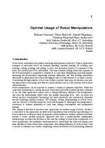
Fig. 2. Experimental setup.

of the ith joint. For an n-jointed manipulator, Eq. (4) can be rewritten as " # n n r X X X δx = Ki + Aqi cos(qθi ) + Bqi sin(qθi ) (5) i=1

q=1

i=1

where r is the number of harmonics. Similar expressions can be written for the position errors of δy, δz. Another alternative polynomial to approximate the error functions with is to employ an ordinary polynomial of the kth degree, which can be expressed as (δx)i = Q i +

k X

j

(Ai θi ).

(6)

j=1

For an n-jointed manipulator, Eq. (6) can be rewritten as " # n n k X X X j δx = Qi + (A ji θi ) . i=1

j=1

(7)

i=1

Again, similar expressions can be written for the position errors of δy, δz. 4. Experimental setup The key elements of the experimental setup depicted in Fig. 2 are the laser tracker unit, retroreflector and the robot manipulator Motoman SK120. The measurement technique used is based on a laser interferometry based tracker (Leica LT500 Laser Tracker) with an accuracy of ∓10 ppm (µm/m), a coordinate repeatability of ∓5 ppm (µm/m) and a distance resolution of 1.26 µm. After the laser tracker has been calibrated to measure the manipulator end point with respect to the manipulator base frame, the manipulator is commanded to 85 different well-spaced positions within the manipulator workspace, which have been determined heuristically to cover the range of motion of all the active joints of the manipulator. We have determined these positions based on the implications reported by Driels and Pathre [9], and Borm and Menq [5] for optimal identification configurations. In order to

G. Alıcı et al. / Robotics and Autonomous Systems 54 (2006) 956–966

959

sition are due to the inaccurate geometrical parameters in the kinematic model described by the entries of the overall transformation matrix in Eq. (2). As we have reported before [1,2], although the best estimates of the parameters are used in the kinematic model and more parameters are subjected to the identification process, there still exist some non-negligible residual positioning errors which need to be eliminated in order to further improve the accuracy of a robotic system. The conventional way of doing this is to consider the effects of all error sources in the identification model such that the resulting identification model is complete in every respect. However, while some of these sources can lead to reproducible systematic errors, many of them cause random errors that differ from one application to another. Therefore, rather than following the conventional way of improving the accuracy of robot manipulators through complete identification models, we suggest a more generic and practical technique to estimate the expected position errors using prediction functions generated by using a Swarm Intelligence based method: Particle Swarm Optimization. These error prediction functions can then be used for estimating the positioning errors without needing further experimental data. The method is systematic and requires four steps for implementation: 1. Choose the type of the polynomial such as a Fourier polynomial, an ordinary polynomial, or any other analytical function, 2. Decide on the size of the function, i.e., the number of coefficients, 3. Estimate the numerical values of the coefficients (by using the PSO method) and also verify the size of the function using experimental data, and 4. Generate a modified joint space or Cartesian space trajectory for error correction.

Fig. 3. The errors of the 85 positions of the manipulator. This identification data was used for generating the error prediction functions.

minimize the effects of measurement noise, the PC based data measurement and recording system of the laser tracker takes 100 measurements for the same configuration and provides the average of these measurements as the measurand. The positional errors of the manipulator for the 85 points are shown in Fig. 3. 5. Particle Swarm Optimization (PSO) method for error prediction Since the measurement system has a very high accuracy [20], it is assumed that the errors in the manipulator’s po-

PSO is a method proposed by Kennedy and Eberhart in 1995 [14]. Their algorithm is inspired by observation of animal foraging behavior, and is based on the metaphor of social interaction. The individuals, as they search the space, are influenced by their own previous behavior and by the successes of their neighbors. The approach to the problem is here similar to one used in genetic algorithms — the system maintains a population of potential solutions (called particles). However in PSO, instead of using genetic operators, the particles “fly” through the problem space following the current “best” particle with some stochastic uncertainty. In this work, we used the basic algorithm [7,14], which can be outlined in the following way. Each particle i is a potential solution xi to a problem in n-dimensional space X . The algorithm is initiated by placing all particles into randomly selected starting positions and the fittest particle ( pibest ) is determined. Each particle maintains a velocity vi as well as its current position xi in X . At every iteration, the best performing particle in the neighborhood is found ( pgbest ), and each particle i adjusts its velocity vi (t + 1) and new position xi (t + 1). Calculations are done for each dimension d (d = 1, . . . , n) by

960

G. Alıcı et al. / Robotics and Autonomous Systems 54 (2006) 956–966

using the following formulas: best vid (t + 1) = vid (t) + c1 × rand( ) × ( pid − xid (t)) best + c2 × rand( ) × ( pgd − xid (t))

the manipulator, the error functions are used to estimate the positioning errors in order to generate modified trajectories for error correction. The error correction procedure is presented in detail in [2].

xid (t + 1) = xid (t) + vid (t + 1) where vid (t) and xid (t) are the current velocity and position best ) is the best position so far, ( p best ) is of the particle i, ( pid gd the position of the best particle in the neighborhood, rand() is a function that returns a uniformly distributed random floating point number ϕ (0 ≤ ϕ ≤ 1) at each call, and c1 = c2 = 2.05 are constants. Calculations are repeated until a termination criterion is met. In our numerical calculations, we used a population size of 100. The fitness (evaluation) function was the RMS (root-mean-square) errors (the PSO algorithm was implemented here as a minimizer). In our case, we stop the iterations when the RMS errors of the generated best particle (over the identification trajectory data, see Fig. 3), drops below a threshold, or the number of iterations reach 200. Each dimension of the n-dimensional space represents the range of possible values a parameter could take. For example, one of our estimator functions, the first degree polynomials with constant coefficients has 15 parameters (Eqs. (15)–(17)) that we attempt to find the best fit values. Therefore, the solution space that our particles (possible solutions) “fly” through has 15 dimensions in this case. The major advantage of Particle Swarm Optimization over other methods such as neural networks, fuzzy interpolation method [26], and in particular genetic algorithms, is its fast convergence. The likelihood of overshooting is minimized because the PSO algorithm in each iteration merely modifies the position of a potential solution in the search hyperspace rather than replacing it with a new solution, as in genetic algorithms. The whole population of PSO moves towards the optimal area and the particles are likely to converge quickly to the best solution. Additionally, PSO is simple and robust, with a small number of parameters that need to be adjusted. 6. Estimation of coefficients of the error prediction functions The procedure of finding the numerical values of the coefficients and the order of the polynomials is to fit a model expressed by either Eq. (5) or Eq. (7) to the error vector 1pk associated with m number of measurements (k = 1 . . . m). 1pk is expressed by   δxk 1pk = δyk  = pr k − pnk (8) δz k where pr k is the kth measured (true), pnk is the corresponding nominal position vector of the kth measurement point, and δxk , δyk , δz k are the resulting position errors in the x, y, and z directions, respectively. The 85 measurements have been used to form the positioning errors and subsequently estimate the coefficients of the error prediction functions. For a given manipulator position or a Cartesian path to be followed by

6.1. Error prediction with angular data The First Degree Polynomials (FDP) with constant coefficients generated by using the PSO method are obtained as δx = 0.46 + 0.48θ1 − 1.25θ2 + 2.64θ3 + 0.86θ6

(9)

δy = 1.90 − 0.63θ1 − 1.32θ2 − 1.30θ3 + 0.46θ6

(10)

δz = −0.85 − 0.67θ1 + 1.08θ2 + 2.72θ3 − 1.50θ6 .

(11)

Similarly, Second Degree Polynomials (SDP) are δx = −0.03 + 0.22θ1 + 0.33θ12 − 1.90θ2 + 1.22θ22 + 3.00θ3 − 1.32θ32 + 0.09θ6 + 0.47θ62 δy = δz =

(12)

−0.28 + 0.47θ1 + 0.65θ12 − 0.58θ2 − 0.43θ22 − 2.35θ3 + 0.79θ32 − 0.34θ6 + 0.28θ62 −2.15 − 0.58θ1 + 0.32θ12 + 1.70θ2 − 0.53θ22 + 1.87θ3 + 0.54θ32 − 1.84θ6 + 0.42θ62 .

(13)

(14)

Since θ4 = θ5 = 0, they do not appear in Eqs. (9)–(14). 6.2. Error prediction with Cartesian data The first degree polynomials with constant coefficients generated by using the PSO method are obtained as δx = 0.73120 − 0.00130 px + 0.00089 p y − 0.00151 pz

(15)

δy = −0.41950 − 0.00130 px − 0.00126 p y + 0.00171 pz (16) δz = 3.00000 + 0.00134 px − 0.00183 p y − 0.00146 pz .

(17)

The second degree polynomials with constant coefficients generated by using the PSO method are obtained as δx = 1.34244 − 0.00126 px − 0.0000002 px2 + 0.00141 p y − 0.0000004 p 2y − 0.00108 pz − 0.0000003 pz2 δy =

−0.41293 − 0.00132 px + 0.00000004 px2 − 0.0000001 p 2y

(18)

− 0.00108 p y

+ 0.00201 pz − 0.0000002 pz2

(19)

δz = 2.06313 + 0.00104 px + 0.0000008 px2 − 0.00217 p y + 0.0000004 p 2y − 0.00221 pz + 0.0000002 pz2 .

(20)

6.3. Interpretation of results A quantitative comparison of the performance of the error prediction functions are presented in Table 2. As one can expect, the RMS errors of each function over the identification trajectory are small. A more reliable indicator of the estimation performance of the functions could be obtained by observing their RMS errors over the test trajectories (on which the functions were not trained on).

961

G. Alıcı et al. / Robotics and Autonomous Systems 54 (2006) 956–966

Table 2 Overall comparison of the prediction performance of the estimator functions: FDP(CI) (Eqs. (15)–(17)) and FDP (Angular Input (AI)) (Eqs. (9)–(11)) are first degree polynomials processing input data in Cartesian and angular formats, similarly SDP (Cartesian Input (CI)) (Eqs. (18)–(20)) and SDP(AI) (Eqs. (12)–(14)) are second degree polynomials, respectively

Uncompen. error FDP(CI) FDP(AI) SDP(CI) SDP(AI)

Root Mean Square (RMS) errors Identification trajectory X Y Z

Test trajectory 1 X Y

Z

Test trajectory 2 X Y

Z

Test trajectory 3 X Y

Z

8.0 2.3 2.0 2.3 1.8

16.2 1.9 4.0 1.5 3.5

16.6 2.9 1.5 2.4 1.3

54.3 2.6 4.9 2.5 5.2

60.9 4.5 0.9 4.2 0.9

11.8 1.8 2.7 1.2 3.0

2.0 1.0 0.6 0.6 1.0

7.5 1.9 1.5 1.9 2.2

17.9 3.3 3.6 3.6 3.6

19.1 1.3 1.0 1.1 1.9

5.4 0.3 0.7 0.3 2.0

19.4 0.5 1.0 0.5 1.8

Fig. 4. The error modeling performance of the error prediction functions over the identification trajectory in the y direction. This result is exemplary in the sense that the modeling performance in the x and z directions are quite similar.

Fig. 5. Test trajectory I: a rectangular path in three-dimensional Cartesian space (left plot), and resulting manipulator joint positions (right plot).

While both Cartesian space and joint space polynomials describe the positioning errors quite well, as seen in Fig. 4 and in Table 2, please bear in mind that the Cartesian space polynomials have the advantages of not needing the inverse kinematics solution, which is tedious and gives multiple solutions. With reference to the results presented in Fig. 4, the PSO method is an alternative to the classical least-square estimation algorithm [2] in determining the coefficients of the mathematical/polynomial models described in the joint space and in the Cartesian space.

The accuracy of the error prediction models can further be improved by dividing the manipulator workspace into subvolumes such that each region is precisely represented with different models/polynomials. For a given Cartesian space trajectory, the appropriate model or a combination of models, if the given trajectory falls into two neighboring sub-regions, is employed to estimate position errors. In principle, the greater number of models is established to estimate positioning errors in various regions of the manipulator workspace, the higher is the success of estimating positioning errors with some mathematical functions.

962

G. Alıcı et al. / Robotics and Autonomous Systems 54 (2006) 956–966

Fig. 6. Test trajectory I: error estimation performance. The first degree polynomial (graphs in the left hand column) and second degree polynomial (graphs in the right hand column) functions using data in Cartesian coordinates.

It must be noted that, instead of the summation of polynomials representing contribution of each joint or each Cartesian direction to the overall Cartesian positioning error, the multiplication of the same polynomials can be used to represent Cartesian positioning errors such that the resulting error model will contain the sum as well as the cross products of the position of all the joints and Cartesian directions. This issue will be investigated and reported later in another publication. We have compared the efficacy of Fourier polynomials and ordinary constant coefficient polynomials in estimating the positioning errors in our previous study based on a classical least-square estimation method [2]. It is found that the Fourier polynomials estimate the positioning errors more accurately than the ordinary polynomials. This outcome will not change with the algorithm employed to estimate the polynomial coefficients. 7. Verification of error prediction functions Three test trajectories have been employed to verify the error estimation method proposed.

This path, with respect to the base coordinate system of the robot, and corresponding joint space trajectory are shown in Fig. 5. It must be noted that the manipulator end point is initially at the location of (1100, 800, 600) mm. Each straight-line part of the path is divided into 50 target points, i.e., the path consists of 200 target points. The error estimation performances of the prediction functions over this rectangular trajectory are shown in Figs. 6 and 7. It must be noted that the Cartesian space polynomials perform better over the joint space polynomials in predicting the positioning errors. One explanation to this finding can be the input motion along the Cartesian directions (x, y, z trajectories) is given as already decoupled motions. On the other hand, the movement of each joint (θ1 · · · θ6 ) contributes to each of the Cartesian error components (δxk , δyk , δz k ) along the Cartesian directions. This results in highly coupled Cartesian error components, which require better approximation functions with many more coefficients. In our previous study, Fourier polynomials with double harmonics and fourth order polynomials, which contain 75 coefficients, have remedied this problem successfully [2].

7.1. Test trajectory I: Rectangular Cartesian path

7.2. Test trajectories II and III: Archimedes spirals

This is a rectangle-like Cartesian path in the threedimensional space of the experimental manipulator considered.

To further verify the validity of the PSO based error modeling technique, two more trajectories were considered.

G. Alıcı et al. / Robotics and Autonomous Systems 54 (2006) 956–966

963

Fig. 7. Test trajectory I: error estimation performance. The first degree polynomial (graphs in the left hand column) and second degree polynomial (graphs in the right hand column) functions using data in angular coordinates.

Fig. 8. Test trajectory II: Archimedes spiral in X –Y plane (left plot), and resulting manipulator joint positions (right plot).

Each of these Cartesian paths is based on an Archimedes spiral defined by r = φ in polar coordinates. The Cartesian coordinates of the spiral are calculated from x = W r cos φ y = W r sin φ

(21) (22)

where φ, the angular position of the radius r from a horizontal 5π axis, is varied from 0 to 5π with a step size of δφ = 200 , and W

is an enlargement factor, its value is chosen as 20. For the test trajectory II, it is assumed that the spiral is given in the X –Y plane, and the z coordinate is changed linearly for 200 target points. The starting coordinate for this trajectory is chosen to be at the point (1200, −600, 600) mm. The path, with respect to the base coordinate system of the robot, and corresponding joint space trajectory are shown in Fig. 8. For test trajectory III, the starting coordinate is decided to be at the point (500,

964

G. Alıcı et al. / Robotics and Autonomous Systems 54 (2006) 956–966

Fig. 9. Test trajectory III: Archimedes spiral in Y –Z plane (left plot), and resulting manipulator joint positions (right plot).

Fig. 10. Test trajectory II: error estimation performance. The first degree polynomial (graphs in the left hand column) and second degree polynomial (graphs in the right hand column) functions using data in Cartesian coordinates.

500, 1400) mm. It is now assumed that the spiral is given in the Y –Z plane, the x coordinate is changed linearly for 200 target points. This path, with respect to the base coordinate system of the robot, and corresponding joint space trajectories are shown in Fig. 9. The error estimation performance of the generated prediction functions over test trajectory II are shown in Figs. 10 and 11. Similar to the finding of test trajectory I, the

Cartesian space polynomials perform better over the joint space polynomials in predicting the positioning errors. By employing better approximation functions such as Fourier polynomials with multiple harmonics or higher-order ordinary polynomials, the error estimation based on the data provided in the joint space can be improved significantly [2]. When the Cartesian position errors estimated through the models presented above are compared to the experimental

G. Alıcı et al. / Robotics and Autonomous Systems 54 (2006) 956–966

965

Fig. 11. Test trajectory II: error estimation performance. The first degree polynomial (graphs in the left hand column) and second degree polynomial (graphs in the right hand column) functions using data in angular coordinates.

(true) errors, it is obvious that the PSO based error prediction technique is valid and can be utilized to estimate the positioning errors of any robot manipulator for the subsequent kinematic error correction process. One important feature of this methodology is that it does not require additional experimental data in order to generate modified joint position trajectories. 8. Conclusions In this paper, we present our study that uses the PSO method to generate functions for predicting expected positioning errors of a robot manipulator. We have generated and tested various estimator functions that use input data in angular space and Cartesian space. Experimental results have been given to demonstrate that the optimization (estimation) models are effective in finding the expected positioning errors without needing further experimental position data for every given trajectory. An overall prediction performance comparison of each function over training (identification) trajectory and test trajectories are given in Table 2. Based on the results, we can claim that the PSO method is a very efficient optimizer that demonstrates fast convergence with a relatively small computational cost, and as such it is a significant step towards the self-calibration of robot manipulators with minimum experimental data.

The results given in this research can further be improved dividing the manipulator workspace into sub-volumes such that each region is precisely represented with different models/polynomials. For a given Cartesian space trajectory, the appropriate model or a combination of models, if the given trajectory falls into two neighboring sub-regions, is employed to estimate position errors. This technique can also be extended to the manipulators with full pose (position and orientation) data available. References [1] G. Alıcı, B. Shirinzadeh, Kinematic identification of a closed-chain manipulator using a laser interferometry based sensing technique, in: Proceedings of the 2003 IEEE/ASME International Conference on Advanced Intelligent Mechatronics, Kobe, Japan, July 2003, pp. 332–337. [2] G. Alıcı, B. Shirinzadeh, A systematic technique to estimate positioning errors for robot accuracy improvement using laser interferometry based sensing, Mechanism and Machine Theory 40 (8) (2005) 879–906. [3] G. Alici, B. Shirinzadeh, Enhanced stiffness modelling, identification and characterisation for robot manipulators, IEEE Transactions on Robotics 21 (4) (2005) 554–564. [4] E. Bonabeau, G. Theraulaz, Swarm Smarts, Scientific American (March) (2000) 72–79. [5] J.H. Borm, C.H. Menq, Determination of optimal measurement configurations for robot calibration based on observability measure, International Journal of Robotics Research 10 (1) (1991) 51–63.

966

G. Alıcı et al. / Robotics and Autonomous Systems 54 (2006) 956–966

[6] H.M. Botee, E. Bonabeau, Evolving ant colony optimization, Advances in Complex Systems 1 (2–3) (1999) 149–159. [7] M. Clerc, J. Kennedy, The particle swarm-explosion, stability, and convergence in a multidimensional complex space, IEEE Transactions on Evolutionary Computation 6 (1) (2002) 58–73. [8] M. Dorigo, V. Maniezzo, A. Coloni, The ant system: optimization by a colony of cooperating agents, IEEE Transactions on Systems, Man and Cybernetics, Part B 26 (1) (1996) 29–41. [9] M.R. Driels, U.S. Pathre, Significance of observation strategy on the design of robot calibration experiments, Journal of Robotic Systems 7 (2) (1990) 197–223. [10] R.P. Dudd, A.B. Knasinski, A technique to calibrate industrial robots with experimental verification, IEEE Transactions on Robotics and Automation 6 (1) (1990) 20–30. [11] J.M. Hollerbach, C.W. Wampler, The calibration index and taxonomy for robot kinematic calibration methods, International Journal of Robotics Research 15 (6) (1996) 573–591. [12] D. Jackson, The Theory of Approximation, vol. XI, Colloquium Publications, American Mathematical Society, 1930. [13] J.H. Jang, S.H. Kim, Y.K. Kwak, Calibration of geometric and nongeometric errors of an industrial robot, Robotica 19 (2001) 311–321. [14] J. Kennedy, R.C. Eberhart, Particle swarm optimization. in: Proceedings of the 1995 IEEE International Conference on Neural Networks, Perth, Australia, 1995, pp. 1942–1948. [15] J. Kennedy, R.C. Eberhart, Swarm Intelligence, Morgan Kaufmann, 2001. [16] W.S. Newman, C.E. Birkhimer, R.J. Horning, A.T. Wilkey, Calibration of a Motoman P8 robot based on laser tracking, in: Proceedings of the 2000 IEEE International Conference on Robotics and Automation, San Francisco, USA, 2000, pp. 3597–3602. [17] J.M. Renders, E. Rossignol, M. Becquet, R. Hanus, Kinematic calibration and geometrical parameter identification for robots, IEEE Transactions on Robotics and Automation 7 (6) (1991) 721–732. [18] L. Sciavicco, B. Siciliano, Modeling and Control of Robot Manipulators, second edn, Springer-Verlag, 2000. [19] G. Szego, Orthogonal Polynomials, vol. XXIII, Colloquium Publications, American Mathematical Society, 1959. [20] P.L. Teoh, B. Shirinzadeh, C.W. Foong, G. Alıcı, The measurement uncertainties in laser interferometry-based sensing and tracking technique, International Journal of Measurement 32 (2) (2002) 135–150. [21] D.E. Whitney, C.A. Lozinski, J.M. Bourke, Industrial robot forward calibration method, ASME Journal of Dynamic Systems, Measurement and Control 108 (1986) 1–8. [22] G. Zak, B. Benhabib, R.G. Fenton, I. Saban, Application of the weighted least squares parameter estimation method to the robot calibration, ASME Journal of Mechanical Design 116 (1994) 890–893. [23] J.S. Shamma, D.E. Whitney, A method for inverse robot calibration, ASME Journal of Dynamic Systems, Measurement and Control 109 (1) (1987) 36–43. [24] B. Benhabib, R.G. Fenton, A.A. Goldenberg, Computer-aided joint error analysis of robots, IEEE Transactions on Robotics and Automation 3 (4) (1987) 317–322. [25] K. Schroer, S.L. Albright, A. Lisounkin, Modeling closed-loop mechanisms in robots for purposes of calibration, IEEE Transactions on Robotics and Automation 13 (4) (1997) 218–229. [26] Y. Bai, D. Wang, Improve the robot calibration accuracy using a dynamic online fuzzy error mapping system, IEEE Transactions on Systems, Man and Cybernetics, Part B (Cybernetics) 34 (1) (2004) 1155–1160.

¨ Dr. Gursel Alıcı received the B.Sc. degree with high honours from Middle East Technical University, Gaziantep, Turkey, in 1988 and the M.Sc. degree from Gaziantep University in 1990 (both degrees in mechanical engineering); and the Ph.D. degree in Robotics from Oxford University, UK, in 1993. He is currently a Senior Lecturer at the School of Mechanical, Materials and Mechatronic Engineering in the University of Wollongong, Australia, where he leads Mechatronic Engineering. His research interests are in the areas of mechanics, optimum design, control and calibration of mechanisms/robot manipulators/parallel manipulators, micro/nano manipulation systems, and modelling, analysis and characterisation of conducting polymer actuators and sensors for use in functional robotic devices. These researches have generated more than 100 fully-refereed international journal and conference papers. Dr. Romuald Jagielski was teaching and researching in a number of universities, among them Gdansk University (Poland) and recently Swinburne University of Technology (Australia) after obtaining his Ph.D. in computer science in 1976. He is now an Honorary Research Associate in the Department of Electrical and Computer Systems Engineering at Monash University. His research interest in artificial intelligence, and in particular in swarm intelligence, is reflected in his publications that comprise conference and journal papers, and two books. Dr. Y. Ahmet S¸ekercio˘glu is a researcher at the Centre for Telecommunications and Information Engineering (CTIE) and a Senior Lecturer in the Electrical and Computer Systems Engineering Department of Monash University. He also holds the position of Program Leader for the Applications Program of Australian Telecommunications Cooperative Research Centre (ATcrc – www.atcrc.com). He has completed his Ph.D. degree at Swinburne University of Technology, and B.Sc. and M.Sc. degrees (all in Electrical and Electronics Engineering) at Middle East Technical University. He has lectured at Swinburne University of Technology for 8 years, and has had numerous positions as a research engineer in private industry. He has published several journal articles, conference papers and two book chapters. His more recent work focuses on development of tools for simulation of large-scale telecommunication networks. He is also interested in application of intelligent control techniques for multiservice networks as complex, distributed systems. Dr. Bijan Shirinzadeh received his BE and MSE in Mechanical and Aerospace Engineering from the University of Michigan, USA, and his Ph.D. in Mechanical Engineering from the University of Western Australia. From 1990 through 1994, he was a senior research scientist in Commonwealth Scientific Industrial Research Organization (CSIRO), Australia. Dr. Bijan Shirinzadeh is currently an Associate Professor, and the Director of Robotics & Mechatronics Research Laboratory (RMRL) which he established in 1994 in the Department of Mechanical Engineering at Monash University, Australia. His current research interests include autonomous systems, sensorybased control, laser-interferometry-based tracking and guidance, micro-nano manipulation systems, virtual reality and haptics, systems kinematics and dynamics, and automated fabrication and manufacturing.