ing to rank, where the task is to learn a ranking model that takes a subset of alternatives as input and ..... The corresponding metric learning problem is formulated as a linear programming problem. 6 ...... IOS Press, 2010. [7] K. Brinker and E.
Preference Learning using the Choquet Integral: The Case of Multipartite Ranking Ali Fallah Tehrani, Weiwei Cheng, Eyke Hüllermeier Department of Mathematics and Computer Science University of Marburg, Germany {fallah, cheng, eyke}@mathematik.uni-marburg.de Draft of a paper to appear in IEEE Transactions on Fuzzy Systems
Abstract We propose a novel method for preference learning or, more specifically, learning to rank, where the task is to learn a ranking model that takes a subset of alternatives as input and produces a ranking of these alternatives as output. Just like in the case of conventional classifier learning, training information is provided in the form of a set of labeled instances, with labels or, say, preference degrees taken from an ordered categorical scale. This setting is known as multipartite ranking in the literature. Our approach is based on the idea of using the (discrete) Choquet integral as an underlying model for representing ranking functions. Being an established aggregation function in fields such as multiple criteria decision making and information fusion, the Choquet integral offers a number of interesting properties that make it attractive from a machine learning perspective, too. The learning problem itself comes down to properly specifying the fuzzy measure on which the Choquet integral is defined. This problem is formalized as a margin maximization problem and solved by means of a cutting plane algorithm. The performance of our method is tested on a number of benchmark datasets. Keywords: preference learning, Choquet integral, classification, monotonicity, attribute interactions
1
Introduction
Preference learning is an emerging subfield of machine learning that has received increasing attention in recent years [18]. Roughly speaking, the goal in preference learning is to induce preference models from observed data that reveals information about the preferences of an individual or a group of individuals in a direct or indirect way; these models
are then used to predict the preferences in a new situation. In this regard, predictions in the form of rankings, i.e., total orders of a set of alternatives, constitute an important special case [13, 30, 19, 16, 20]. A ranking can be seen as a specific type of structured output [3], and compared to conventional classification and regression functions, models producing such outputs require a more complex internal representation. In this paper, we propose a novel method for such kind of ranking problems, for the first time using the (discrete) Choquet integral [12] as an underlying model for representing rankings in a setting of supervised learning. The Choquet integral is an established aggregation function that has been used in various fields of application, including multiple criteria decision making and information fusion. It can be seen as a generalization of the weighted arithmetic mean that is not only able to capture the importance of individual features but also information about the interaction (e.g., redundancy or complementarity) between different features. Moreover, it obeys monotonicity properties in a rather natural way. Due to these properties, the Choquet integral appears to be very appealing for preference learning, especially for aggregating the evaluation of individual features in the form of interacting criteria. The learning problem itself comes down to specifying the fuzzy measure underlying the definition of the Choquet integral in the most suitable way. In this regard, we explore connections to kernel-based machine learning methods [48]. While a number of different types of ranking problems have been introduced in the literature in recent years, we specifically focus on a setting referred to as multipartite ranking [13, 20]. Roughly speaking, the task in multipartite ranking is to learn a ranking model that takes any set of alternatives as input, with each alternative typically represented in terms of a feature vector, and produces a ranking of these alternatives as output. Just like in the case of conventional classifier learning, training information is provided in the form of a set of labeled instances, with labels or, say, preference degrees taken from an ordered categorical scale (such as bad, good, very good). The remainder of this paper is organized as follows. In the next section, we give a brief overview of related work. In Section 3, we recall the basic definition of the (discrete) Choquet integral and related notions. The ranking problem we are dealing with and our method for tackling this problem are introduced in Sections 4 and 5, respectively. Experimental results are presented in Section 6, prior to concluding the paper in Section 7.
2
Related Work
In this section, we briefly review related work on preference learning and the use of the Choquet integral in machine learning.
2
2.1
Preference Learning
Methods for the automatic learning, discovery and adaptation of preferences have received increasing interest in machine learning, data mining and related research fields in recent years. Approaches relevant to this area range from preference elicitation where the utility function of a single agent is estimated by asking questions effectively [8, 27, 52] to collaborative filtering where a customer’s preferences are estimated from the preferences of other customers [44, 45]. Preference learning can be formalized within various settings, depending, e.g., on the underlying preference model and the type of information provided as an input to the learning system. There are two main approaches to modeling preferences that prevail in the literature on choice and decision theory: value functions and preference relations. From a machine learning point of view, these two approaches give rise to two kinds of learning problems: learning value functions and learning (binary) preference relations. The latter deviates more strongly than the former from conventional problems like classification and regression, as it involves the prediction of complex structures, such as rankings or partial order relations, rather than single values. Moreover, training input in preference learning will not, as it is usually the case in supervised learning, be offered in the form of complete examples but may comprise more general types of information, such as relative preferences or different kinds of indirect feedback and implicit preference information [36, 47]. In general, a preference learning system is provided with a set of items (e.g., products) for which preferences are known, and the task is to learn a function that predicts preferences for a new set of items (e.g., new products not seen so far), or for the same set of items in a different context (e.g., the same products but for a different user). Frequently, the predicted preference relation is required to form a total order, in which case we also speak of a ranking problem. In fact, among the problems in the realm of preference learning, the task of “learning to rank” has probably received the most attention in the literature so far, and a number of different ranking problems have already been introduced. Based on the type of training data and the required predictions, Fürnkranz and Hüllermeier [18] distinguish between the problems of object ranking [13, 38], label ranking [7, 29, 10, 51] and instance ranking [20, 46]. All of these basic learning tasks can be tackled by similar techniques. As with the distinction between using value functions and binary relations for modeling preferences, two general approaches to preference learning have been proposed in the literature, the first one being based on the idea of learning to evaluate individual alternatives by means of a value function, while the second one seeks to compare (pairs of) competing alternatives, that is, to learn one or more binary preference predicates. Making sufficiently restrictive model assumptions about the structure of a preference relation, one can also
3
try to use the data for identifying this structure. Finally, local estimation techniques à la nearest neighbor can be used, which mostly leads to aggregating preferences in one way or another. A value function assigns an abstract degree of utility to each alternative under consideration. Depending on the underlying utility scale, which is typically either numerical or ordinal, the problem of learning a (latent) value function from given training data becomes one of regression learning or ordinal classification. Both problems are well-known in machine learning. However, value functions often implicate special requirements and constraints that have to be taken into consideration such as, for example, monotonicity in certain attributes. Besides, as mentioned earlier, training data is not necessarily given in the form of input/output pairs, i.e., alternatives (instances) together with their utility degrees, but may also consist of qualitative feedback in the form of pairwise comparisons, stating that one alternative is preferred to another one and therefore has a higher utility degree. In general, this means that value functions need to be learned from indirect instead of direct training information [36, 47]. The learning of binary preference relations that compare alternatives in a pairwise manner is normally simpler, mainly because comparative training information (suggesting that one alternative is better than another one) can be used directly instead of translating it into constraints on a (latent) value function [19, 35]. On the other hand, the prediction step may become more difficult, since a binary preference relation learned from data is not necessarily consistent in the sense of being transitive and, therefore, does normally not define a ranking in a unique way. What is needed, therefore, is a ranking procedure that maps a preference relation to a maximally consistent ranking [33]. The difficulty of this problem depends on the concrete consistency criterion used, though many natural objectives (e.g., minimizing the number of object pairs whose ranks are in conflict with their pairwise preference) lead to NP-hard problems [13]. Fortunately, efficient techniques such as simple voting (known as the Borda count procedure in social choice theory) often deliver good approximations, sometimes even with provable guarantees [14, 34]. Another approach to learning ranking functions is to proceed from specific model assumptions, that is, assumptions about the structure of the preference relations. This approach is less generic than the previous ones, as it strongly depends on the concrete assumptions made. An example is the assumption that the target ranking of a set of objects described in terms of multiple attributes can be represented as a lexicographic order [17, 54, 6]. Another example is the assumption that the target ranking can be represented by a CP-net [11]. From a machine learning point of view, assumptions of the above type can be seen as an inductive bias restricting the hypothesis space. Provided the bias is correct, this is clearly an advantage, as it may simplify the learning problem considerably. 4
Yet another alternative is to resort to the idea of local estimation techniques as prominently represented, for example, by the nearest neighbor estimation principle [15, 32]: Considering the rankings observed in similar situations as representative, a ranking for the current situation is estimated on the basis of these “neighbored” rankings, typically using an averaging-like aggregation operator [7, 9]. This approach is in a sense orthogonal to the previous model-based one, as it is very flexible and typically comes with no specific model assumption (except the regularity assumption underlying the nearest neighbor inference principle).
2.2
The Choquet Integral in Machine Learning
Although the Choquet integral has been widely applied as an aggregation operator in multiple criteria decision making [23, 21, 50] and as a tool for preference elicitation [1, 2], it has been used much less in the field of machine learning so far. There are, however, a few notable exceptions. Methods for binary classification based on the Choquet integral were developed in [26] and [55]. In [26], Grabisch essentially employs the Choquet integral as a fusion operator (j) in this context. For an instance x = (x1 , . . . , xn ), let φi (x) express a measure of confidence (provided by feature i) that x belongs to class j ∈ {0, 1}. Grabisch defines the global confidence for class j as an aggregation of these confidence degrees: � � df (j) , φµ(j) (x) = Cµ(j) φ1 (x), . . . , φ(j) n (x) where Cµ denotes the discrete Choquet integral with respect to the fuzzy measure µ. Eventually, the class with the highest global confidence is predicted as an output. Here, the fuzzy measures µ(0) and µ(1) express the importance of the features and groups of (j) features in the classification process. The φi are assumed to be derived by means of a conventional parametric or nonparametric probability density estimation method, subsequent to suitable normalization. The identification of the fusion operator is then reduced to the identification (or learning) of the fuzzy measures µ(0) and µ(1) with 2(2n − 2) coefficients. To this end, Grabisch minimizes the empirical squared error loss J=
X�
�2 φµ(0) (x) − φµ(1) (x) − 1 +
x∈T0
X�
φµ(1) (x) − φµ(0) (x) − 1
�2
(1) ,
x∈T1
i.e., the sum of squared differences between predicted and given output values, using standard optimization routines (T0 and T1 denote, respectively, the set of observed negative and positive examples). Yan, Wang and Chen [55] tackle a quite similar problem, albeit using another optimization criterion (which can be seen as a kind of relaxed class 5
separability criterion). Besides, the authors define the Choquet integral based on a so-called signed non-additive measure [41]. Apart from binary classification, the Choquet integral was also used in ordinal classification, a special type of multi-class classification in which the class labels are linearly ordered (e.g., a paper submitted for publication can be labeled as accept, weak accept, weak reject, or reject). Grabisch [25, 24] considers input data of the following kind: A reference set of objects A = {1, . . . , l} and a set of criteria X = {1, . . . , n}; a table of individual scores (performances) zki (k ∈ A, i ∈ X); a partial preorder ≥A on A (partial ranking of the objects on a global basis); a partial preorder ≥X on X (partial ranking of the criteria); a partial preorder ≥P on the set of pairs of criteria (partial ranking of interaction); the sign of interaction between selected pairs of criteria, reflecting synergy, independence or redundancy. All this information can be translated into linear equalities or inequalities between the weights of the underlying fuzzy measure µ. This measure is then identified based on a constraint optimization problem, using as objective function a criterion that resembles very much the so-called margin principle in machine learning. The method itself, however, is more oriented towards decision making and less suitable for machine learning applications. In particular, it is not tolerant toward noise in the data and, in terms of complexity, does not scale well with the size of the data. In [4], Beliakov and James develop a method for classifying journals in the field of pure mathematics, which are rated on an ordinal scale with categories A+ , A, B and C. The classification is done on the basis of five criteria serving as input attributes, namely the number of citations per year, the impact factor, the immediacy index, the total number of articles published, and the cited half-life index (we shall use the same data set in our experiments later on). As a loss function, the authors use the absolute difference between the predicted class and the target (i.e., the loss is |i − j| if the i-th class is predicted although the j-th class would be correct). Although our focus in this paper is on the use of the Choquet integral in supervised learning, it is worth mentioning that it can also be used in other settings. In the recent paper [5] by Beliakov et al., the discrete Choquet integral is used for metric learning in semi-supervised clustering. The authors investigate necessary and sufficient conditions for the discrete Choquet integral to define a metric, and, as a special case, obtain analogous conditions for ordered weighted averaging (OWA) operators. The corresponding metric learning problem is formulated as a linear programming problem.
6
3
The Discrete Choquet Integral
In this section, we give a brief introduction to the (discrete) Choquet integral, starting with a reminder of non-additive measures. In contrast to other fields, such as decision making and aggregation operators, the Choquet integral is not widely known in machine learning so far, which is the main reason to recall its definition in some detail. Readers familiar with the Choquet integral and related notions can safely skip this section.
3.1
Non-Additive Measures
Let X = {x1 , . . . , xn } be a finite set and µ a measure 2X → [0, 1]. For each A ⊆ X, we interpret µ(A) as the weight or, say, the importance of the set of elements A. As an illustration, one may think of X as a set of criteria (binary features) relevant for a job, like “speaking French” and “programming Java”, and of µ(A) as the evaluation of a candidate satisfying criteria A (and not satisfying X \ A). The term “criterion” is indeed often used in the decision making literature, where it suggests a monotone “the higher the better” influence. A standard assumption on a measure µ(·), which is, for example, at the core of probability theory, is additivity: µ(A ∪ B) = µ(A) + µ(B) for all A, B ⊆ X such that A ∩ B = ∅. Unfortunately, additive measures cannot model any kind of interaction between elements: Extending a set of elements A ⊆ X by a set of elements B ⊆ X \ A always increases the weight µ(A) by the weight µ(B), regardless of A and B. Suppose, for example, that the elements of two sets A and B are complementary in a certain sense. For instance, A = {French, Spanish} and B = {Java} could be seen as complementary, since both language skills and programming skills are important for the job. Formally, this can be expressed in terms of a positive interaction: µ(A ∪ B) > µ(A) + µ(B). In the extreme case, when language skills and programming skills are indeed essential, µ(A ∪ B) can be high although µ(A) = µ(B) = 0 (suggesting that a candidate lacking either language or programming skills is completely unacceptable). Likewise, elements can interact in a negative way: If two sets A and B are partly redundant or competitive, then µ(A ∪ B) < µ(A) + µ(B). For example, B = {Java} and C = {C, C#} might be seen as redundant, since knowledge of one programming language does in principle suffice. The above considerations motivate the use of non-additive measures, also called capacities or fuzzy measures, which are simply normalized and monotone: µ(∅) = 0, µ(X) = 1, and µ(A) ≤ µ(B) for all A ⊆ B ⊆ X .
(2)
A useful representation of non-additive measures, that we shall explore later on for 7
learning Choquet integrals, is in terms of the Möbius transform: X µ(B) = m(A)
(3)
A⊆B
for all B ⊆ X, where the Möbius transform mµ of the measure µ is defined as follows: X mµ (A) = (−1)|A|−|B| µ(B) . (4) B⊆A
The value mµ (A) can be interpreted as the weight that is exclusively allocated to A, instead of being indirectly connected with A through the interaction with other subsets. A measure µ is said to be k-order additive, or simply k-additive, if k is the smallest integer such that m(A) = 0 for all A ⊆ X with |A| > k. This property is interesting for several reasons. First, as can be seen from (3), it means that a measure µ can formally be specified by significantly fewer than 2n values, which are needed in the general case. Second, k-additivity is also interesting from a semantic point of view: As will become clear in the following, this property simply means that there are no interaction effects between subsets A, B ⊆ X whose cardinality exceeds k.
3.2
Importance of Criteria and Interaction
An additive (i.e., k-additive with k = 1) measure µ can be written as follows: X X µ(A) = µ({xi }) = wi , xi ∈A
xi ∈A
with wi = µ({xi }) the weight of xi . Due to (2), these weights are non-negative and such P that ni=1 wi = 1. In this case, there is obviously no interaction between the criteria xi , i.e., the influence of an xi on the value of µ is independent of the presence or absence of any other xj . Besides, the weight wi is a natural quantification of the importance of xi . Measuring the importance of a criterion xi becomes obviously more involved when µ is non-additive. Besides, one may then also be interested in a measure of interaction between the criteria, either pairwise or even of a higher order. In the literature, measures of that kind have been proposed, both for the importance of single as well as the interaction between several criteria. Given a fuzzy measure µ on X, the Shapley value (or importance index) of xi is defined as a kind of average increase in importance due to adding xi to another subset A ⊂ X: � � X 1 ! µ(A ∪ {xi }) − µ(A) . (5) ϕ(xi ) = n − 1 A⊆X\{xi } n |A| 8
The Shapley value of µ is the vector ϕ(µ) = (ϕ(x1 ), . . . , ϕ(xn )). One can show that P 0 ≤ ϕ(xi ) ≤ 1 and ni=1 ϕ(xi ) = 1. Thus, ϕ(xi ) is a measure of the relative importance of xi . Obviously, ϕ(xi ) = µ({xi }) if µ is additive. The interaction index between criteria xi and xj , as proposed by Murofushi and Soneda [40], is defined as follows: � X ϑA · µ(A ∪ {xi , xj }) − µ(A ∪ {xi }) I(xi , xj ) = A⊆X\{xi ,xj }
� −µ(A ∪ {xj }) + µ(A) , with
1
ϑA =
n−2 |A|
(n − 1)
!.
This index ranges between −1 and 1 and indicates a positive (negative) interaction between criteria xi and xj if Ii,j > 0 (Ii,j < 0). The interaction index can also be expressed in terms of the Möbius transform: � � X 1 m {xi , xj } ∪ K . I(xi , xj ) = k+1 K⊆X\{xi ,xj },|K|=k
Furthermore, as proposed by Grabisch [22], the definition of interaction can be extended to more than two criteria, i.e., to subsets T ⊆ X: n−|T |
I(T ) =
X k=0
3.3
1 k+1
X
� � m T ∪K .
K⊆X\T,|K|=k
The Choquet Integral
So far, the criteria xi were simply considered as binary features, which are either present or absent. Mathematically, µ(A) can thus also be seen as an integral of the indicator function of A, namely the function fA given by fA (x) = 1 if x ∈ A and = 0 otherwise. Now, suppose that f : X → R+ is any non-negative function that assigns a value to each criterion xi ; for example, f (xi ) might be the degree to which a candidate satisfies criterion xi . An important question, then, is how to aggregate the evaluations of individual criteria, i.e., the values f (xi ), into an overall evaluation, in which the criteria are properly weighted according to the measure µ. Mathematically, this overall evaluation can be considered as an integral Cµ (f ) of the function f with respect to the measure µ. Indeed, if µ is an additive measure, the standard integral just corresponds to the weighted mean n n X X Cµ (f ) = wi · f (xi ) = µ({xi }) · f (xi ) , (6) i=1
i=1
9
which is a natural aggregation operator in this case. A non-trivial question, however, is how to generalize (6) in the case where µ is non-additive. This question, namely how to define the integral of a function with respect to a nonadditive measure (not necessarily restricted to the discrete case), is answered in a satisfactory way by the Choquet integral, which has first been proposed for additive measures by Vitali [53] and later on for non-additive measures by Choquet [12]. The point of departure of the Choquet integral is an alternative representation of the “area” under the function f , which, in the additive case, is a natural interpretation of the integral. Roughly speaking, this representation decomposes the area in a “horizontal” instead of a “vertical” manner, thereby making it amenable to a straightforward extension to the non-additive case. More specifically, note that the weighted mean can be expressed as follows: n X
= =
f (xi ) · µ({xi })
i=1 n � X i=1 n � X
� � � f (x(i) ) − f (x(i−1) ) · µ({x(i) }) + . . . + µ({x(n) }) � � � f (x(i) ) − f (x(i−1) ) · µ A(i) ,
i=1
where (·) is a permutation of {1, . . . , n} such that 0 ≤ f (x(1) ) ≤ f (x(2) ) ≤ . . . ≤ f (x(n) ) (and f (x(0) ) = 0 by definition), and A(i) = {x(i) , . . . , x(n) }. Now, the key difference between the left and right-hand side of the above expression is that, whereas the measure µ is only evaluated on single elements xi on the left, it is evaluated on subsets of elements on the right. Thus, the right-hand side suggests an immediate extension to the case of non-additive measures, namely the Choquet integral, which, in the discrete case, is formally defined as follows: Cµ (f ) =
n X
� f (x(i) ) − f (x(i−1) ) · µ(A(i) ) .
i=1
In terms of the Möbius transform of µ, the Choquet integral can also be expressed as
10
follows: Cµ (f ) = = =
n X i=1 n X i=1 n X
� f (x(i) ) − f (x(i−1) ) · µ(A(i) ) f (x(i) ) · (µ(A(i) ) − µ(A(i+1) )) f (x(i) )
X
m(R)
i=1
R⊆T(i)
X
m(T ) × min f (xi )
=
xi ∈T
T ⊆X
(7)
� where T(i) = S ∪ {x(i) } | S ⊂ {x(i+1) , . . . , x(n) } . Note that the expression (7) can also be written in terms of an inner product D E mϕ , ϕ(f (x)) , with the mapping ϕ : Rn → R2
n −1
defined as follows:
ϕ(x) = ϕ(x1 , . . . , xn ) � = x1 , . . . , xn , min{x1 , x2 }, . . . , min{xn−1 , xn }, � min{x1 , x2 , x3 }, . . . , min{x1 , . . . , xn } . Moreover, mϕ denotes the vector (m1 , . . . , mn , mn+1 , . . . , m2n −1 ) of values of the Möbius transform in the order determined by ϕ(x).
4
Multipartite Ranking
As mentioned earlier, different types of ranking problems have recently been studied in the machine learning literature. Here, we are specifically interested in the so-called multipartitle ranking problem [20]. In most ranking problems, the goal is to learn a ranking function that accepts a subset O ⊂ O of objects as input, where O is a reference set of objects (e.g., the set of all books or movies). As output, the function produces a ranking (total order) � of the objects O. Typically, a ranking function of that kind is implemented by means of a scoring function U : O → R, so that o � o0
⇔
U (o) ≥ U (o0 )
for all o, o0 ∈ O. Obviously, U (o) can be considered as a kind of utility degree assigned to the object o ∈ O. Seen from this point of view, the goal in multipartite ranking is to 11
learn a latent utility function on a reference set O. In the following, we shall also refer to U (·) itself as a ranking function. Moreover, we assume that this function produces a strict order relation �, i.e., ties U (o) = U (o0 ) do not occur or are broken at random. In order to induce a ranking function U (·), a learning algorithm (or “learner” for short) is provided with training information. In the case of multipartite ranking, the “ground truth” is supposed to be an ordinal categorization of objects. That is, each object o ∈ O belongs to one of the classes in L = {λ1 , λ2 , . . . , λk }, where the classes are sorted such that λ1 < λ2 < . . . < λk . Correspondingly, training data consists of a set of labeled objects (oi , `i ) ∈ O × L, just like in ordinal regression. The goal is to learn a ranking function U (·) that agrees well with the sorting of the classes in the sense that objects from higher classes are ranked higher than objects from lower classes. In [20], it was proposed to use the so-called C-index as a performance measure reflecting this goal in an adequate way: P P 0 1≤i k. In fact, choosing a k � n is not only interesting from an optimization but also from a learning point of view: Since the degree of additivity of µ offers a way to control the capacity of the underlying model class, selecting a proper k is crucial in order to guarantee the generalization performance of the learning algorithm. More specifically, the larger k is chosen, the more flexibly the Choquet integral can be fitted to the data. Thus, choosing k too large comes along with a danger of overfitting the data.
5.2
Dealing with Soft Margin Constraints
The number of soft margin constraints (11–12) may become quite large, too, as it scales quadratically with the size N of the training data. To cope with the complexity implied by these constraints, we refer to the idea underlying cutting plane algorithms, which originates from linear optimization theory and has already been used successfully in learning support vector machines for classification [37]. The key idea of cutting plane algorithms is to solve the problem by considering only a subset of all constraints, hoping that the rest will be satisfied, too. If this is not the 14
Algorithm 1 Cutting plane algorithm 1: Input: training set S = {(fi1 j1 , y1 ), ..., (fiK jK , yK )} ⊂ [−1, +1]n × {−1, +1}, ζ, � 2: W = ∅ 3: repeat 4: (w, ξ) ← arg minw,ξ≥0 12 w> w + ζξ s.t. 5: ∀(y 1 , . . . , y K ) ∈ W : P PK w> · K k=1 ∆(yk , y k ) [ψ(fik jk , yk ) − ψ(fik jk , y k )] ≥ k=1 ∆(yk , y k ) − Kξ Pn ∗ ∗ ∗ ∗ ∗ 6: w · (φ(Z ) − φ(Z)) ≤ 0 for all Z ∈ Sl−1 , Z ∈ Sl s. t. k=1 zk − zk = 1 (1 ≤ l ≤ n) 7: for k = 1 to K do � � 8: y˜k ← arg maxy˜∈{−1,+1} ∆(yk , y˜) 1 − w> · [ψ(fik jk , yk ) − ψ(fik jk , y˜)] 9: end for 10: W ← W ∪ {(˜ y1 , . . . , y˜K )} 11: until P PK ˜k )[ψ(fik jk , yk ) − ψ(fik jk , y˜k )] ≤ Kξ + K� ˜k ) − w> · K k=1 ∆(yk , y k=1 ∆(yk , y 12: return(w,ξ) 1 13: mφ = P2n −1 ·w k=1
wk
case, then more constraints are added. More concretely, most algorithms start with an empty set of constraints and successively add the constraint that is maximally violated by the current solution. The pseudo-code of the cutting plane approach is shown in Algorithm 1. For each pair of objects (oi , oj ) ∈ D with oi � oj , we denote by fij the difference foi − foj , to which we assign the class label +1; conversely, fji = foj − foi is assigned the class label −1. The function ψ is defined as ψ(x, y) = φ(x)y, where y ∈ {−1, +1}. Moreover, ∆ is a loss function defined as ( 0 y=y , (16) ∆(y, y) = L otherwise where L is a rescaling parameter that can be set to 1 without loss of generality. Roughly speaking, the lower L, the stronger the slack ξ is penalized; the importance of the slack in the objective function is controlled by the parameter ζ. Finally, Sl∗ = {(z1 , . . . , zn ) ∈ P {0, 1}n | ni=1 zi = l }, where n is the number of features and l ∈ {1, . . . , n}. As can be seen, the algorithm iteratively constructs a working set W = W1 ∪ . . . ∪ Wr of constraints, starting with an empty set W = ∅. In each step, the algorithm finds the constraint that is mostly violated by the current solution w, ξ and adds it to the working set. Additionally, it guarantees the monotonicity constraints; the formulation in line 6 is provably equivalent to the inequality constraints (15). The algorithm terminates as soon as no further constraints are violated by more than the predefined precision �. 15
Table 1: Data sets and their properties data set Color (CLR) 1–7 Scientific Journals (SCJ) CPU Auto MPG Employee Selection (ESL) Mamographic (MMG) Lecturers Evaluation (LEV) Concrete Compressive Strength (CCS) Car Evaluation (CEV)
6
#instances 120 172 209 398 488 830 1000 1030 1728
#attributes 3 5 6 8 4 5 4 8 6
#classes 3 4 2 6 9 2 5 6 4
source [43] [4] UCI UCI WEKA UCI WEKA UCI UCI
Experimental Results
6.1
Data
Preference learning data meeting the requirements of our setting is by far not as abundant as data for standard machine learning problems such as classification and regression. In particular, note that we require data in which the output is measured on an ordered categorical scale. Moreover, since the Choquet integral is a monotone aggregation operator, the data should be monotone in the sense that the output can be expected to increase with each input attribute. In total, we managed to collect 15 data sets meeting these requirements, mainly from the UCI repository1 and the WEKA machine learning framework [28]. These are all benchmark data sets commonly used for experimental purposes in machine learning. Besides, we collected a number of real-world data sets from other sources, namely data from an industrial polyester dyeing process [42] and data about the evaluation of mathematical journals [4]. Table 1 provides a summary of all data sets, which can be downloaded from our website.2 In what follows, we give a brief description of these data sets. • Color: The first data set is color yield. It originates from an industrial polyester dyeing process that was also analyzed in [43]. Here, the output variable is the color yield, which has been measured as a function of three important factors of the production process: disperse dyes concentration, temperature and time of dyeing. Corresponding experiments have been made for seven different colors, giving rise to seven data sets. Since the output variable is actually numeric, we turn it into an ordinal class variable with three values; to this end, two thresholds are defined in such a way that the class distribution is uniform. 1 2
http://archive.ics.uci.edu/ml/ http://www.uni-marburg.de/fb12/kebi/research/
16
• Scientific Journals: This data set is comprised of journals in the field of pure mathematics, which are rated on a scale with categories A+ , A, B and C [4]. Each journal is moreover scored in terms of 5 criteria serving as input attributes, namely, cites (the total number of citations per year), the impact factor (average number of citations per article within two years after publication), the immediacy index (cites to articles in current calendar year divided by the number of articles published in that year), articles (the total number of articles published), and cited half-life (median age of articles cited). • CPU: This is a standard benchmark data set from the UCI repository. It contains nine attributes, three of which were removed since they are obviously of no predictive value (vendor name, model name, ERP). • Auto MPG: This data set contains eight attributes and one output. The attributes are cylinders, displacement, horsepower, weight, acceleration, model year, origin, car name. The last attribute (car name) was removed because it has no predictive value. The output is fuel consumption in miles per gallon (MPG). In order to obtain an ordinal class structure, the MPG value was discretized into six consecutive intervals. • Employee Selection: This data set contains profiles of applicants for certain industrial jobs. The values of the four input attributes were determined by psychologists based upon psychometric test results and interviews with the candidates. The output is an overall score on an ordinal scale between 1 and 9, corresponding to the degree of suitability for each candidate to this type of job. • Mammographic: This data set is about breast cancer screening by mammography. The goal is to predict the severity (benign or malignant) of a mammographic mass lesion from BI-RADS attributes (mass shape, mass margin, density) and the patient’s age. • Lecturers Evaluation: This data set contains examples of anonymous lecturer evaluations, taken at the end of MBA courses. Students were asked to score their lecturers according to four attributes such as oral skills and contribution to their professional/general knowledge. The output was a total evaluation of each lecturer’s performance, measured on an ordinal scale from 0 to 4. • Concrete Compressive Strength: This data set comprises 8 quantitative input variables, namely the following features of concrete: cement, blast furnace slag, fly ash, water, superplasticizer, coarse aggregate, fine aggregate, age. The output set is the concrete compressive strength measured in megapascal. We turned it into an ordinal attribute using equi-width binning with 6 bins.
17
• Car Evaluation: This data set contains 6 attributes describing a car: buying price, price of the maintenance, number of doors, capacity in terms of persons to carry, the size of luggage boot, estimated safety of the car. The output is the overall evaluation of the car: unacceptable, acceptable, good, very good.
6.2
Comparison with Linear and Polynomial Kernel Methods
We compared our approach (subsequently referred to as CI) with kernel-based methods for ranking, using the spider implementation3 of the RankSVM approach with a linear and a polynomial kernel [31]. A comparison with this class of methods is interesting for several reasons. First, kernel-based methods belong to the state-of-the-art in the field of learning to rank. Second, they make use of the same type of learning algorithm (large margin maximization). Third, the use of a polynomial kernel leads to a model that bears some resemblance with a Choquet integral. In fact, using a polynomial kernel of degree d on the original feature representation of objects, i.e., a kernel of the form K(o, o0 ) = (hfo , fo0 i + λ)d ,
(17)
essentially comes down to fitting a linear model in an expanded feature space, in which the original features f (x1 ), . . . , f (xn ) are complemented by all monomials of order ≤ d. Thus, a polynomial kernel of degree d captures the same level of interactions between criteria as a Choquet integral on a k-additive fuzzy measure, when k = d. Note, however, that it does not guarantee monotonicity in the input attributes. Moreover, we compared with the weighted mean (WM), which does indeed assure monotonicity, but which is not able to capture any interaction between variables. This model was implemented as a special case of our method, namely the case of the Choquet integral based on a 1-additive measure.
6.3
Experimental Setup
In order to assure commensurability [39], all features were normalized to the range 0 and 1 before learning, thereby turning them into a criterion, i.e., a “the higher the better” attribute. To this end, the transformation fo (xi ) = (xi − mi )/(Mi − mi ) was used, where mi and Mi are, respectively, the lower and upper bounds for xi (estimated from the data); if the influence of xi is actually negative, the mapping fo (xi ) = (Mi − xi )/(Mi − mi ) is used instead. We randomly split the data into two parts, one half for training and one half for testing. In order to find the trade-off parameter γ, we conducted a 5-fold cross validation on the training data, selecting an optimal γ from {10−4 , 10−3 , 10−2 , 10−1 , 1, 10, 102 , 103 }. The 3
http://people.kyb.tuebingen.mpg.de/spider/
18
Table 2: Performance in terms of the average C-index ± standard deviation. Additionally, the rank of each method it shown in brackets. data set CLR 1 CLR 2 CLR 3 CLR 4 CLR 5 CLR 6 CLR 7 SCJ CPU MPG ESL MMG LEV CCS CEV average rank
WM .9663±.0148(4) .8740±.0293(4) .9343±.0204(4) .9357±.0171(4) .9518±.0194(3) .9046±.0202(4) .8880±.0312(4) .8168±.0105(4) .9965±.0027(3) .8887±.0176(4) .9497±.0162(2) .8961±.0230(2) .8710±.0289(2) .8650±.0068(4) .8981±.0066(4) 3.47
PL d=1 .9506±.0155(5) .8601±.0294(5) .9268±.0219(5) .9228±.0247(5) .9485±.0179(5) .8923±.0205(5) .8797±.0256(5) .8098±.0112(5) .9950±.0093(5) .8850±.0143(5) .9559±.0071(1) .8536±.0168(4) .8620±.0320(3) .8586±.0102(5) .8804±.0076(5) 4.53
PL d=2 .9674±.0129(3) .8876±.0200(3) .9375±.0156(3) .9431±.0189(3) .9565±.0142(2) .9127±.0201(3) .8892±.0219(3) .8270±.0241(3) .9978±.0012(2) .8912±.0078(3) .9465±.0104(4) .8714±.0181(3) .8713±.0250(1) .8862±.0184(3) .9118±.0059(3) 2.8
PL d=3 .9700±.0141(2) .9341±.0244(2) .9633±.0143(2) .9659±.0166(2) .9516±.0171(4) .9460±.0191(2) .9258±.0237(2) .8313±.0109(2) .9955±.0005(4) .8967±.0093(2) .9491±.0126(3) .7813±.0350(5) .8527±.0300(5) .8962±.0203(2) .9585±.0090(2) 2.73
CI .9828±.0090(1) .9804±.0128(1) .9878±.0150(1) .9915±.0056(1) .9682±.0140(1) .9825±.0121(1) .9688±.0167(1) .8450±.0201(1) .9986±.0014(1) .9060±.0111(1) .9424±.0098(5) .9015±.0210(1) .8610±.0320(4) .9050±.0038(1) .9771±.0039(1) 1.47
model induced from the training data is then evaluated on the test data, measuring performance in terms of the C-index. This procedure was repeated 100 times, and the results were averaged.
6.4
Results
An overview of the results is given in Table 2. Moreover, Table 3 provides a summary in terms of win-loss statistics, showing, for each pair of methods, on how many data sets the first one is better than the second one. The overall picture conveyed by the results is clearly in favor of our method. In fact, the superiority of CI can also be corroborated statistically, noting that 12 wins is enough to reject the null-hypothesis of equal performance according to a simple (two-tailed) sign test at the 5% significance level. Statistically, the results thus suggest that CI is signifiantly better than the competitor methods. Table 4 shows results for our method when restricting the Choquet integral to k-additive measures, for different values of k. A restriction of this kind is interesting for several reasons. First, since less parameters need to be estimated, it reduces complexity and, therefore, increases the efficiency of our learning algorithm. Second, as already explained earlier, a restriction to k-additive measures is also interesting from a learning (induction) point of view, as it allows for controlling the capacity of the underlying hypothesis space: The larger the value of k, the richer the model space becomes. In other words, k can be used to control the flexibility (non-linearity) of the model class. If k is too small, the model is not able to fit the data sufficiently well. On the other hand, if k is too large,
19
Table 3: Win statistics (number of data sets on which the first method was better than the second one) WM PL d=1 PL d=2 PL d=3 CI WM – 14 2 5 2 PL d=1 1 – 1 3 2 PL d=2 13 14 – 4 2 PL d=3 10 12 11 – 1 CI 13 13 13 14 –
Table 4: C-index for restriction to k-additive measures (best result highlighted in bold). data set CLR 1 CLR 2 CLR 3 CLR 4 CLR 5 CLR 6 CLR 7 SCJ CPU MPG ESL MMG LEV CCS CEV
CI k=2 .9825±.0103 .9803±.0095 .9874±.0101 .9921±.0063 .9683±.0141 .9867±.0120 .9665±.0162 .8459±.0245 .9986±.0009 .9038±.0136 .9486±.0172 .8941±.0290 .8667±.0216 .9149±.0131 .9411±.0082
CI k=3 .9828±.0090 .9804±.0128 .9878±.0150 .9915±.0056 .9682±.0140 .9825±.0121 .9688±.0167 .8447±.0201 .9985±.0016 .9044±.0111 .9457±.0176 .8960±.0217 .8635±.0241 .9123±.0155 .9660±.0066
CI k=4 ——– ——– ——– ——– ——– ——– ——– .8458±.0191 .9988±.0010 .9049±.0104 .9424±.0098 .8964±.0172 .8610±.0320 .9120±.0184 .9670±.0053
CI k=5 ——– ——– ——– ——– ——– ——– ——– .8450±.0201 .9984±.0011 .9058±.0093 ——– .9015±.0210 ——– .9104±.0104 .9678±.0041
CI k=6 ——– ——– ——– ——– ——– ——– ——– ——– .9986±.0014 .9060±.0111 ——– ——– ——– .9050±.0038 .9771±.0039
there is a danger of over-fitting the data, which may lead to poor generalization. Ideally, k is chosen so as to avoid both problems, namely under- and over-fitting the data. As can be seen in Table 4, the ideal value does indeed depend on the data set and is often smaller than the largest possible value (namely k = #attributes). The question of how to determine an optimal value of k in an efficient way (i.e., without simply trying all alternatives) is an important topic of future work. As one of the key features of our approach, we already mentioned the aspect of interpretability. In particular, the Choquet integral (or, more specifically, the underlying fuzzy measure) provides natural measures of the importance of individual and the interaction between pairs (or even groups) of attributes. As an illustration, Fig. 1 visualizes the (pairwise) interaction between attributes for the car evaluation data, for which CI performs significantly better than WM. Recall that, in this data set, the evaluation of 20
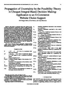
a car (output attribute) depends on a number of criteria, namely (a) buying price, (b) price of the maintenance, (c) number of doors, (d) capacity in terms of persons to carry, (e) size of luggage boot, (f) safety of the car. These criteria form a natural hierarchy: (a) and (b) form a subgroup PRICE, whereas the other properties are of a TECHNICAL nature and can be further decomposed into COMFORT (c–e) and safety (f). Interestingly, the interaction in our model nicely agrees with this hierarchy: Interaction within each subgroup tends to be smaller (as can be seen from the darker colors) than interaction between criteria from different subgroups, suggesting a kind of redundancy in the former and complementarity in the latter case. In addition, Fig. 2 visualizes the interaction between the three attributes in the color yield data sets, namely for CLR-1 and CLR-7. The interaction is not very strong in the case of CLR-1, but more pronounced for CLR-7. This is in agreement with the improvement achieved by CI in comparison with a simple linear model (WM), which is relatively small in the former but much higher in the latter case. In fact, it is plausible that a complex, non-linear model like CI is not needed unless the attributes are strongly interacting. Or, stated differently, if there is (almost) no interaction between the attributes, a simple linear model will generally be enough.
Figure 1: Visualization of the interaction index for the car evaluation data (numerical values are shown in terms of level of gray, values on the diagonal are set to 0). Groups of related criteria are indicated by the black lines.
7
Summary and Conclusions
In this paper, we have advocated the use of the discrete Choquet integral in the context of preference learning. More specifically, we have used the Choquet integral for representing a latent utility function in multipartite ranking, a specific type of preference 21
1
1 TE
TE 0.5
TI
0.5
0
0
TI
−0.5
−0.5
CO
CO TI
TE
CO
−1 TI
TE
CO
−1
Figure 2: Visualization of the interaction index for data sets CLR-1 (left) and CLR-7 (right). The reduction of prediction error is about twice as much as for CLR-7. For the ease of representation, the values on the diagonal are set to 0. learning problem. This idea is motivated by several appealing properties offered by the Choquet integral, making it quite attractive from a preference learning point of view. This includes its ability to capture dependencies between criteria (attributes) and to obey natural monotonicity conditions, as well as its interpretability. In fact, in preference learning, one is often not only interested in the prediction of preferences. Instead, it may also be important to get an explanation of a prediction, i.e., a reason for why an alternative A is (presumably) preferred to another alternative B. The measures of importance and interaction between attributes, which can directly be derived from the fuzzy measure underlying the Choquet integral, provide extremely valuable information in this regard. The proper specification of this measure, i.e., the adaptation of the fuzzy measure to the data at hand, is the main challenge from a machine learning point of view. We formalized this problem as a (soft) margin maximization problem and solved it by means of a cutting plane algorithm. Our algorithm was compared to state-of-the-art ranking methods on a number of benchmark datasets. The results of these experiments are very promising and clearly in favor of our approach. Needless to say, the method proposed in this paper can be refined in several directions. Especially interesting in this regard is the idea of restricting the model class to kadditive measures, connected with the use of k as a kind of regularization parameter (cf. Section 6). Moreover, going beyond the specific problem of multipartite ranking, one may of course also think of applying the Choquet integral to other types of preference learning problems. Indeed, being convinced of the high potential of this idea, we consider this paper as a first step toward establishing the Choquet integral as an important mathematical tool of preference learning, and a precursor for research along similar lines.
22
Acknowledgments: This work was supported by the German Research Foundation (DFG). We thank Maryam Nasiri (University of Siegen, Germany) and Gleb Beliakov (Deakin University, Australia) for providing us the color yield data and the journal data, respectively.
References [1] Silvia Angilella, Salvatore Greco, and Benedetto Matarazzo. Non-additive robust ordinal regression with Choquet integral, bipolar and level dependent Choquet integrals. In Joao Paulo Carvalho, Didier Dubois, Uzay Kaymak, and Joao Miguel da Costa Sousa, editors, Proceedings of the Joint International Fuzzy Systems Association World Congress and European Society of Fuzzy Logic and Technology Conference, pages 1194–1199. IFSA/EUSFLAT, 2009. [2] Silvia Angilella, Salvatore Greco, and Benedetto Matarazzo. Non-additive robust ordinal regression: A multiple criteria decision model based on the Choquet integral. European Journal of Operational Research, 201:277–288, 2010. [3] G. Bakir, T. Hofmann, B. Schölkopf, A. Smola, B. Taskar, and S. Vishwanathan, editors. Predicting Structured Data. The MIT Press, 2007. [4] Gleb Beliakov and Simon James. Citation-based journal ranks: the use of fuzzy measures. Fuzzy Sets and Systems, 167(1):101–119, 2011. [5] Gleb Beliakov, Simon James, and Gang Li. Learning Choquet-integral-based metrics for semisupervised clustering. IEEE Transactions on Fuzzy Systems, 19(3):562– 574, 2011. [6] R. Booth, Y. Chevaleyre, J. Lang, J. Mengin, and C. Sombattheera. Learning conditionally lexicographic preference relations. In H. Coelho, R. Studer, and M. Wooldridge, editors, Proceedings of the 19th European Conferece on Artificial Intelligence, pages 269–274. IOS Press, 2010. [7] K. Brinker and E. Hüllermeier. Case-based label ranking. In Johannes Fürnkranz, Tobias Scheffer, and Myra Spiliopoulou, editors, Proceedings of the European Conference on Machine Learning and Principles and Practice of Knowledge Discovery in Databases, pages 566–573. Springer, 2006. [8] U. Chajewska, L. Getoor, J. Norman, and Y. Shahar. Utility elicitation as a classification problem. In Gregory Cooper and Serafin Moral, editors, Proceedings of the 14th Conference on Uncertainty in Artificial Intelligence, pages 79–88. Morgan Kaufmann, 1998.
23
[9] W. Cheng, K. Dembczyński, and E. Hüllermeier. Label ranking based on the Placket-Luce model. In J. Fürnkranz and T. Joachims, editors, Proceedings of the 27th International Conference on Machine Learning, pages 215–222. Omnipress, 2010. [10] W. Cheng, J. Hühn, and E. Hüllermeier. Decision tree and instance-based learning for label ranking. In Andrea Pohoreckyj Danyluk, Léon Bottou, and Michael L. Littman, editors, Proceedings of the 26th International Conference on Machine Learning, pages 161–168. Omnipress, 2009. [11] Y. Chevaleyre, F. Koriche, J. Lang, J. Mengin, and B. Zanuttini. Learning ordinal preferences on multiattribute domains: the case of CP-nets. In J. Furnkranz and E. Hüllermeier, editors, Preference Learning, pages 273–296. Springer, 2010. [12] Gustave Choquet. Theory of capacities. Annales de l’institut Fourier, 5:131–295, 1954. [13] William Cohen, Robert Schapire, and Yoram Singer. Learning to order things. Journal of Artificial Intelligence Research, 10(1):243–270, 1999. [14] D. Coppersmith, L. Fleischer, and A. Rudra. Ordering by weighted number of wins gives a good ranking for weighted tournaments. ACM Transactions on Algorithms, 6(3):55:1–55:13, 2010. [15] T.M. Cover and P.E. Hart. Nearest neighbor pattern classification. IEEE Transactions on Information Theory, IT-13:21–27, 1967. [16] Ofer Dekel, Christopher Manning, and Yoram Singer. Log-linear models for label ranking. In Sebastian Thrun, Lawrence Saul, and Bernhard Schölkopf, editors, Advances in Neural Information Processing Systems, volume 16. The MIT Press, 2003. [17] P. Flach and T. Matsubari. A simple lexicographic ranker and probability estimator. In Joost Kok, Jacek Koronacki, Ramon López de Mántaras, Stan Matwin, Dunja Mladenic, and Andrzej Skowron, editors, Proceedings of the European Conference on Machine Learning and Principles and Practice of Knowledge Discovery in Databases, pages 575–582. Springer, 2007. [18] J. Fürnkranz and E. Hüllermeier, editors. Preference Learning. Springer, 2010. [19] Johannes Fürnkranz and Eyke Hüllermeier. Pairwise preference learning and ranking. In Nada Lavrac, Dragan Gamberger, Ljupco Todorovski, and Hendrik Blockeel, editors, Proceedings of the European Conference on Machine Learning and Principles and Practice of Knowledge Discovery in Databases, pages 145–156. Springer, 2003. 24
[20] Johannes Fürnkranz, Eyke Hüllermeier, and Stijn Vanderlooy. Binary decomposition methods for multipartite ranking. In Wray Buntine, Marko Grobelnik, Dunja Mladenic, and John Shawe-Taylor, editors, Proceedings of the European Conference on Machine Learning and Principles and Practice of Knowledge Discovery in Databases, pages 359–374. Springer, 2009. [21] Michel Grabisch. Fuzzy integral in multicriteria decision making. Fuzzy Sets and Systems, 69(3):279–298, 1995. [22] Michel Grabisch. k-order additive discrete fuzzy measures and their representation. Fuzzy Sets and Systems, 92(2):167–189, 1997. [23] Michel Grabisch. Fuzzy integral for classification and feature extraction. In Michel Grabisch, Toshiaki Murofushi, and Michio Sugeno, editors, Fuzzy Measures and Integrals: Theory and Applications, pages 415–434. Physica, 2000. [24] Michel Grabisch, Ivan Kojadinovic, and Patrick Meyer. A review of methods for capacity identification in Choquet integral based multi-attribute utility theory: Applications of the Kappalab R package. European Journal of Operational Research, 186(2):766–785, 2008. [25] Michel Grabisch, Toshiaki Murofushi, and Michio Sugeno, editors. Fuzzy Measures and Integrals: Theory and Applications. Physica, 2000. [26] Michel Grabisch and Marc Roubens. Application of the Choquet integral in multicriteria decision making. In Michel Grabisch, Toshiaki Murofushi, and Michio Sugeno, editors, Fuzzy Measures and Integrals: Theory and Applications, pages 348–374. Physica, 2000. [27] P. Haddawy, V. Ha, A. Restificar, B. Geisler, and J. Miyamoto. Preference elicitation via theory refinement. Journal of Machine Learning Research, 4:317–337, 2003. [28] Mark Hall, Eibe Frank, Geoffrey Holmes, Bernhard Pfahringer, Peter Reutemann, and Ian H. Witten. The WEKA data mining software: an update. ACM SIGKDD Explorations Newsletter, 11(1):10–18, 2009. [29] S. Har-Peled, D. Roth, and D. Zimak. Constraint classification: a new approach to multiclass classification. In Nicolò Cesa-Bianchi, Masayuki Numao, and Rüdiger Reischuk, editors, Proceedings of the 13th International Conference on Algorithmic Learning Theory, pages 365–379. Springer, 2002. [30] Sariel Har-Peled, Dan Roth, and Dav Zimak. Constraint classification for multiclass classification and ranking. In Suzanna Becker, Sebastian Thrun, and Klaus Ober-
25
mayer, editors, Advances in Neural Information Processing Systems, volume 15, pages 785–792. The MIT Press, 2003. [31] Ralf Herbrich, Thore Graepel, and Klaus Obermayer. Large margin rank boundaries for ordinal regression. In Alexander Smola, Peter Bartlett, Bernhard Schölkopf, and D. Schuurmans, editors, Advances in Large Margin Classifiers, pages 115–132. The MIT Press, 2000. [32] E. Hüllermeier. Similarity-based inference as evidential reasoning. International Journal of Approximate Reasoning, 26:67–100, 2001. [33] E. Hüllermeier and J. Fürnkranz. Comparison of ranking procedures in pairwise preference learning. In IPMU–04, 10th International Conference on Information Processing and Management of Uncertainty in Knowledge-Based Systems, Perugia, Italy, 2004. [34] E. Hüllermeier and J. Fürnkranz. On predictive accuracy and risk minimization in pairwise label ranking. Journal of Computer and System Sciences, 76(1):49–62, 2010. [35] Eyke Hüllermeier, Johannes Fürnkranz, Weiwei Cheng, and K. Brinker. Label ranking by learning pairwise preferences. Artificial Intelligence, 172:1897–1917, 2008. [36] T. Joachims. Optimizing search engines using clickthrough data. In Proceedings of the 8th ACM SIGKDD International Conference on Knowledge Discovery and Data Mining, pages 133–142. ACM, 2002. [37] Thorsten Joachims, Thomas Finley, and Chun-Nam John Yu. Cutting-plane training of structural SVM. Machine Learning, 77(1):27–59, 2009. [38] T. Kamishima, H. Kazawa, and S. Akaho. A survey and empirical comparison of object ranking methods. In J. Fürnkranz and E. Hüllermeier, editors, Preference Learning, pages 181–202. Springer, 2010. [39] Francois Modave and Michel Grabisch. Preference representation by a Choquet integral: commensurability hypothesis. In Bernadette Bouchon-Meunier and Ronald Yager, editors, Proceedings of the 7th International Conference on Information Processing and Management of Uncertainty in Knowledge-Based Systems, pages 164–171. Editions EDK, 1998. [40] Toshiaki Murofushi and S. Soneda. Techniques for reading fuzzy measures (III): interaction index. In Proceedings of the 9th Fuzzy Systems Symposium, pages 693– 696, 1993.
26
[41] Toshiaki Murofushi, Michio Sugeno, and Motoya Machida. Non-monotonic fuzzy measures and the Choquet integral. Fuzzy Sets and Systems, 64(1):73–86, 1994. [42] Maryam Nasiri. Fuzzy regression modeling of colour yield in dyeing polyester with disperse dyes. Master’s thesis, Textile Engineering Department, Isfahan University of Technology, 2003. [43] Maryam Nasiri and Stefan Berlik. Modeling of polyester dyeing using an evolutionary fuzzy system. In Joao Paulo Carvalho, Didier Dubois, Uzay Kaymak, and Joao Miguel da Costa Sousa, editors, Proceedings of the Joint International Fuzzy Systems Association World Congress and European Society of Fuzzy Logic and Technology Conference, pages 1246–1251. IFSA/EUSFLAT, 2009. [44] M.J. Pazzani. A framework for collaborative, content-based and demographic filtering. Artificial Intelligence Review, 13(5–6):393–408, 1999. [45] P. Perny and J.D. Zucker. Preference-based search and machine learning for collaborative filtering: the “film-conseil” movie recommender system. Information, Interaction, Intelligence, 1(1):9–48, 2003. [46] J.R. Quevedo, E. Montanes, O. Luaces, and J.J. del Coz. Adapting decision DAGs for multipartite ranking. In José Balcázar, Francesco Bonchi, Aristides Gionis, and Michèle Sebag, editors, Proceedings of the European Conference on Machine Learning and Principles and Practice of Knowledge Discovery in Databases, pages 115–130. Springer, 2010. [47] F. Radlinski and T. Joachims. Query chains: learning to rank from implicit feedback. In Robert Grossman, Roberto Bayardo, and Kristin Bennett, editors, Proceedings of the 11th ACM SIGKDD International Conference on Knowledge Discovery and Data Mining, pages 239–248. ACM, 2005. [48] Bernhard Schölkopf and Alexander Smola. Learning with Kernels: Support Vector Machines, Regularization, Optimization, and Beyond. The MIT Press, 2001. [49] A. Fallah Tehrani, W. Cheng, K. Dembczynski, and E. Hüllermeier. Learning monotone nonlinear models using the Choquet integral. In Proceedings of the European Conference on Machine Learning and Principles and Practice of Knowledge Discovery in Databases. Springer, 2011. [50] Vicenc Torra. Learning aggregation operators for preference modeling. In Johannes Fürnkranz and Eyke Hüllermeier, editors, Preference Learning, pages 317–333. Springer, 2011. [51] S. Vembu and T. Gärtner. Label ranking: a survey. In J. Fürnkranz and E. Hüllermeier, editors, Preference Learning, pages 45–64. Springer, 2010. 27
[52] P. Viappiani, P. Pu, and B. Faltings. Preference-based search with adaptive recommendations. AI Communications - Recommender Systems, 21(2–3):155–175, 2008. [53] Giuseppe Vitali. Sulla definizione di integrale delle funzioni di una variabile. Annali di Matematica Pura ed Applicata, 2(1):111–121, 1925. [54] F. Yaman, T.J. Walsh, M.L. Littman, and M. des Jardins. Democratic approximation of lexicographic preference models. In William W. Cohen, Andrew McCallum, and Sam T. Roweis, editors, Proceedings of the 25th International Conference on Machine Learning, pages 1200–1207. ACM, 2008. [55] Nian Yan, Zhenyuan Wang, and Zhengxin Chen. Classification with Choquet integral with respect to signed non-additive measure. In G. Jagannathan and R. Wright, editors, Proceedings of the 7th IEEE International Conference on Data Mining Workshops, pages 283–288. IEEE, 2007.
28