PRELIMINARY GOODNESS-OF-FIT TESTS FOR NORMALITY DO NOT VALIDATE THE ONE-SAMPLE STUDENT t
William R. Schucany and H. K. Tony Ng Department of Statistical Science Southern Methodist University Dallas, Texas 75275-0332
[email protected] Key Words: adaptive procedure, nonparametric, permutation, Monte Carlo simulation, pretest, robustness, Shapiro-Wilk. Running head: Preliminary Goodness-of-fit Tests. AMS Classification: Primary 62F03; Secondary 62A01. ABSTRACT One of the most basic topics in many introductory statistical methods texts is inference for a population mean, µ. The primary tool for confidence intervals and tests is the Student t sampling distribution. Although the derivation requires independent identically distributed normal random variables with constant variance, σ 2 , most authors reassure the readers about some robustness to the normality and constant variance assumptions. Some point out that if one is concerned about assumptions, one may statistically test these prior to reliance on the Student t. Most software packages provide optional test results for both (a) the Gaussian assumption and (b) homogeneity of variance. Many textbooks advise only informal graphical assessments, such as certain scatterplots for independence, others for constant variance, and normal quantile-quantile plots for the adequacy of the Gaussian model. We concur with this recommendation. As convincing evidence against formal tests of (a), such as the Shapiro-Wilk, we offer a simulation study of the tails of the resulting conditional sampling distributions of the Studentized mean. We analyze the results of systematically screening all samples from normal, uniform, exponential, and Cauchy populations. This 1
pretest does not correct the erroneous significance levels and makes matters worse for the exponential. In practice we conclude that graphical diagnostics are better than a formal pretest. Furthermore, rank or permutation methods are recommended for exact validity in the symmetric case. 1. INTRODUCTION Is it ever a good idea to test for normality before using a sample X1 , X2 , . . . , Xn to make inferences about a mean, µ, relying upon the Student t sampling distribution? Most software packages provide optional test results for (a) the Gaussian assumption (e.g. SAS, PROC UNIVARIATE) and (b) homogeneity of variance (e.g. SAS, PROC TTEST; SPSS, The Independent-Samples t Test procedure). Good textbooks on statistical methodology, e.g. Ramsey and Shafer (2002), argue against formal preliminary tests and favor informal graphical diagnostics. These applied statistics texts advise only graphical assessments, such as certain scatterplots for independence, others for constant variance, and normal quantilequantile plots for the adequacy of the Gaussian model. We support this recommendation with concrete evidence for the case that formal tests of (a), as recommended by Romeu (2003), are actually flawed. In teaching beginning courses we find it useful to address this basic point directly. For paired data and multiple samples the issues are different. Suppose this random sample of size n is from a distribution F with population mean, µ. A statistical practice that is possible in many packages is to first use a goodness-of-fit (GOF) test for normality, i.e. H0∗ : The true F is normal against H1∗ : F is not normal
(1)
at the level of significance αg before making inference based on the t-statistic. If one does not reject H0∗ , one treats the sample as coming from a normal distribution and uses the Student t-statistic T =
n n ¯ − µ0 X 1 X X ¯ = 1 ¯ 2, √ , where X Xi and s2 = (Xi − X) s/ n n i=1 n − 1 i=1
2
to test the hypothesis H0 : µ = µ0 against H1 : µ 6= µ0
(2)
at the level of significance αt . In order to assess the adequacy of the preliminary GOF tests for normality, we compare the true Type-I error rate given that the sample passed this pretest, i.e. α = Pr(Reject H0 |do not reject H0∗ and H0 is true),
(3)
to the pre-specified nominal Type-I error rate, αt . Thoughtful readers recognize a logical problem here. The nominal level, αt , requires that H0∗ be true but in (3) one is only given that H0∗ was not rejected. Consequently, hoping for this two-stage procedure to work puts one in the ill-advised position of accepting a narrow null hypothesis. Strictly speaking, this null of normality is not simple, but it is one quite special family in the space of all continuous distributions. On the parallel issue (b) of common variance, preliminary testing of σ12 = σ22 has a more extensive literature. The Behrens-Fisher problem has been troublesome for decades. A fresh approach that does not pretest (b) is given by Sprott and Farewell (1993). Their position agrees well with ours that “a procedure, based on accepting the null hypothesis, seems logically flawed.” They give a collection of confidence intervals for a difference between two means that adapt to the statistical evidence on the ratio σ22/σ12 . There is a sizable literature on GOF and much of it pertains to tests for normality or a few other specific families. There is a growing consensus that neither the chi-square (Moore, 1986, p.91) nor the Kolmogorov-Smirnov can be recommended due to the superiority of many others based on moments, probability plots, or other empirical distribution function (EDF) tests. Tukey (1993, p.31) stated that “The Kolmogoroff-Smirnov construction . . . is logically correct, but practically almost useless.” He cited Michael (1983) for a transformation better suited to the sup norm. For this reason we concentrate only on the Shapiro-Wilk statistic, W (Shapiro and Wilk, 1965) and the EDF Anderson-Darling statistic, A2 (Stephens, 1974) 3
for normality. See D’Agostino and Stephens (1986) for definitions, theory, and efficiency comparisons in finite samples. Because we find the results using these two pretests to be very similar, we only report those for W , which essentially tests for linearity in normal quantile-quantile plots. 2. A SIMULATION OF THE EFFECTS OF A PRELIMINARY TEST The algorithm for our Monte Carlo study follows. Step 1. Simulate a random sample of size n from a distribution F . Step 2. Use the Shapiro-Wilk statistic, W , to test for normality (1), at the level of significance αg with the International Mathematical and Statistical Libraries (IMSL) function DSPWLK (Visual Numerics, Inc., 1994). Step 3. If H0∗ is not rejected in Step 2, treat the sample as coming from a normal distribution and use the t-test of the hypothesis (2) at the level of significance αt. If H0∗ is rejected in Step 2, then return to Step 1. In this simulation experiment we consider sample sizes n = 10, 20, 30, and 50; and the following underlying distributions F , (i) uniform (0, 1), µ0 = 0.5, (ii) standard exponential, µ0 = 1.0, (iii) Cauchy, median = 0.0, (iv) standard normal, µ0 = 0.0. There are four fixed levels of significance for the preliminary GOF test αg = 10%, 5%, 1%, and 0.5% and crossed with four levels of significance for the t-test αt = 10%, 5%, 1%, and 0.5%. For each combination of n, αg , αt and F , we independently repeat Steps 1 through 3 until H0∗ is not rejected M = 100, 000 times. Hence this inverse sampling yields 100,000 samples that have passed our normality screening. Then the Type-I error rate in (3) for the t-test is estimated by α ˆ=
number of times H0 (2) is rejected . M
(4)
Easterling and Anderson (1978) report a similar Monte Carlo study of n = 10, 20, αg = 10%, and M = 1000. They employ the chi-square (12 bins for deciles and 5th and 4
95th percentiles) to assess the resulting agreement with the entire Student t sampling distributions. We focus on the relevant feature of the quantiles for inference at four conventional levels, e.g. 90% confidence. Our greater precision allows us to reach stronger conclusions. We also gain some valuable insight on the sensitivity to pretest levels down to αg = 0.5%. Even though the t-test is not justifiable for the Cauchy, it is useful to assess its performance. 3. RESULTS OF SCREENING OUT NONNORMAL SAMPLES Tables 1 - 5 in the Appendix summarize the Type-I error rates for four pretest levels αg and without any pretest, four conventional levels of significance, αt , and four different underlying distributions in our experiment. These Type-I error rates are estimated from 100,000 replications of the Student t-statistic. The standard errors (SE) at each of the nominal levels are at the head of each respective column. This final power column has a maximum SE = 0.12% because of the negative binomial stopping rule to produce 100,000 acceptable samples. The number of simulated samples to produce 100,000 samples passing Shapiro-Wilk pretest can be obtained from this final power column. For example in Table 3 (αg = 1%), when F is the exponential and n = 10, the simulated power of Shapiro-Wilk test is 23.4%, implying implies 100000/(1 - 0.234) = 130,548 samples to produce 100,000 passing the GOF pretest. When F is Gaussian, as one might hope, the preliminary GOF test does no harm whenever the data are truly normally distributed. When the underlying distributions are nonnormal, one might hope that the preliminary goodness-of-fit tests screen out the blatantly non-normal samples and correct the Type-I error rates for the t-test. However, our results show this not to be the case in general. To demonstrate the effect of the pretest on the Type-I error rate for the t-test, Figure 1 plot the independent estimates (4) for the t-test at αt = 5% after passing Shapiro-Wilk tests at αg = 10%, 5%, 1%, 0.5%, and also with no GOF test. Some interesting interactions are apparent. From Figure 1a, when F is Cauchy, we see that for sample sizes from 10 to 50 the GOF screens yield somewhat better results (simulated Type-I error rates closer to the nominal level) than applying the t-test without any pretest. For example, at n = 30 and αt = 5%, 5
the true Type-I error rate improved from 2.0% to 3.7% (SE =0.07%). However, the simulated Type-I error rates are still significantly less than the nominal αt for every n is our study. The absence of any effect of n is consistent with the theory for the Cauchy. Multiple comparisons are protected at each n. The vertical bars at each plotting symbol are 95% family-wise Tukey-corrected intervals for the 10 pairwise differences among the five rates. For displays of such intervals see Mason, Gunst and Hess (2003) Section 6.5. [Figure 1 about here] The genuinely noteworthy effect is that the pretest actually makes matters worse for both the uniform and the exponential. That is, for these two populations the true Type-I error rates are closer to the nominal αt when one uses the t-test on every sample, rather than selectively using only those samples with acceptable preliminary GOF statistics. From Figure 1b, when the underlying distribution is uniform, GOF tests at αg = 1% and 0.5% corrected the problem for small sample sizes (n = 10 and 20). However, for large sample sizes, the true Type-I error rates for the t-test without the GOF pretest are closer to the nominal αt . For example at n = 50 and αt = 5% the estimated Type-I error rates with preliminary GOF tests are around 4.2% to 4.4%, while the rate without any pretest is 5.0% (from Table 5, SE =0.07%). This can be explained by the rapid convergence to normality of the mean of samples from the symmetric short-tailed uniform distribution. The degradation of the conditional test is due to increasing power and corresponding greater selectivity for samples with relatively long tails. From Figure 1c when the underlying distribution is exponential, preliminary GOF tests not only do not help bring the conditional Type-I error rates closer to the nominal level, they actually makes matters worse than no pretest. This is especially so when the sample sizes are large. This is our “smoking gun” evidence. For example at n = 50 and αt = 5% the estimated Type-I error rate with preliminary goodness-of-fit tests at αg = 0.5% is 16.2% (from Table 4) while the estimated rate without is 6.5% (from Table 5, SE =0.07%). Somewhat surprisingly, when the sample size increases, the conditional Type-I error rates increase, getting further away from the nominal rate, αt . It appears to be quite detrimental to use the GOF test of
6
normality before applying the t-test, because they yield actual Type-I error rates that are much greater than the nominal level. The reason is subtle. What is being detected is a changing selection effect on the conditional mean value. Even though we are likely to detect these skewed distributions in large samples, for small n = 10 the αg = 5% level tests let about 56% of the samples be treated as normal. Graphical evidence that even Anderson-Darling pretests do no harm to the normal may be seen in Figure 2a. Using A2 at αg = 10% for n = 10 selects about 90% of normal samples with relatively light tails. Consequently, one might suspect a distortion of some features of the subsequent t(9) sampling distribution. There is no evidence of any such selection bias in Q-Q plots of 10,000 Student t with 9 degrees of freedom. On the other hand in Figure 2b, the disparity is quite obvious, when we subject the exponential to the same process. [Figure 2 about here] 4. OTHER VALID INFERENCE PROCEDURES In practice, reliable inference on means, when there is convincing evidence of nonnormality, takes two or more non-Student paths. The issues are different for skewed and symmetric alternatives. Our symmetric nonnormals, the Cauchy and the uniform, represent relatively heavier- and lighter-tailed symmetric alternatives, respectively. For both of these, one might consider using the Wilcoxon signed-rank or a permutation distribution (Ernst, 2004) either (i) on the rejected samples or (ii) on all samples from the outset. We offer a portion of a larger simulation study that strongly suggests that (ii) is the recommended strategy. Table 6 summarizes two analyses of M = 100, 000 samples of size n = 10 for only one nominal level αt = 5%. The empirical levels in the table for both distributions are subject to a simulation SE = .07%. In contrast to the approach in Section 3, we assess the Type-I error rates incurred by the adaptive procedure with the t-test on “accepted” samples and distribution-free procedures on the “rejected” ones. The two-sided Wilcoxon-signed rank is exact of size 4.88% (see Lehmann, 1998). The exact conditional permutation distribution has 210 = 1, 024 points. Thus, its true level can be closer to 5%. What is evident in Table 6 is that the validity of the t-test is not repaired for the Cauchy 7
and the uniform by resorting to either of these distribution-free tests on the significantly non-normal samples. As we know, it does control Type-I error rates exactly to use either Wilcoxon or permutation tests on every sample with no pretesting. However, the net result of the two stages in (i) can be significantly different than the nominal level. For instance the Shapiro-Wilk at αg = 1% yields a combined level for the t/Wilcoxon of 4.52% (t/Permutation of 4.58%) for the Cauchy, which is detected about 48% of the time. These are significantly less than 5% with exact binomial two-sided p-values < 10−9 . The corresponding results for the uniform, t/Wilcoxon of 5.42%, (t/Permutation of 5.48%) are significantly greater with p-values < 10−9 . The effect of αg is in the anticipated direction. That is, larger αg yield greater power, which improves the approximation to αt . However, the important conclusion is that none of these two-stage procedures have the desired validity, which is present in the appropriate rank or permutation test with no pretest (option (ii)). On the other hand more refined adaptive tests can produce satisfactory increases in power for paired samples, see Freidlin, Miao and Gastwirth (2003). We analyzed these same procedures at n = 20, 30 and 50 as well as for other levels αt = .10, .01 and .005. The patterns were consistent with the ones for n = 10 and αt = 5%; although the effect of αg was less pronounced at n = 50 for the Cauchy, where the corresponding powers were .996, .993, .987, and .984. The proper handling of skewed alternatives is much more difficult. If conditions are right for the lognormal, then the log transformation is ideal. However, other right-skewed families, such as exponential, gamma, Weibull, Gumbel, inverse Gaussian, and Pareto, are not perfectly symmetrized by the logs, reciprocals, or square roots, which tend to be used in practice. The fundamental problem comes from trying to make inference on the mean of any skewed distribution. When these are paired differences, symmetry is a natural result. When there are two independent samples, permutation tests permit inference on shift parameters without requiring normality or even symmetry. Therefore, the one-sample location problem
8
for skewed families is not as well posed as when µ is the center of symmetry. All of the other inferences about comparisons are reasonably well handled by permutation tests. We recommend that they be used in parallel with t-tools and not only whenever the sample appears to be nonnormal. 5. CONCLUSIONS AND DISCUSSIONS There are some apparently counterintuitive results in Section 3. If one does any preliminary test of H0∗ , it appears best to use a very small level, e.g., αg = 0.5%. This may seem to refute many analysts’ experience with GOF tests, which have notoriously low power in small to moderate sample sizes. Hence, it may seem that one would argue for αg = 10% to have any chance of screening out the Cauchy or the exponential. Even though our intuition may be right about the power of these tests, it fails us whenever we imagine that the Student t approximation is conditionally better, when one rejects more of the exponential samples. This can be seen in Figure 1c that the exponential is best with no preliminary tests. The pretest’s selection effect on the conditional mean depends on both αg and n. Based on the results here, we recommend that one use formal GOF tests of normality before applying the t-test with great caution, especially when the underlying population distribution is suspected to be skewed. This precaution holds for any other tests like F tests, that are sensitive to nonnormality. When the sample size is reasonably large, say n ≥ 50, the central limit theorem supports the Student t approximation and any pretest is ill-advised. If one wishes to use the GOF test of normality, we suggest fixing the level of significance at a very low level, say αg = 0.1%. Diagnostic plots and tests should guide us to transform clearly nonnormal data. When nonnormality is blatant in such graphics, it may be a surrogate for p < .001 in a test. Obviously, the same conclusion holds for confidence intervals. The inaccuracies that we demonstrate in each tail of the conditional sampling distributions have precisely the same effect on the coverage probabilities of one- or two-sided intervals for µ. Easterling (1976) described a simultaneous inferential procedure for both the distributional model and its parameters. In practice for the one-sample problem our recommendation is to use t-tests and intervals 9
along with permutation methods. As a standard part of the diagnostics, the next stage should include normal quantile-quantile or log density (Hazelton, 2003) plots. Whenever these (or GOF tests) have strong evidence of obvious nonnormality, one should rely on the tests and intervals from rank-based and permutation distributions or look for satisfactory transformations for improved inference on µ. This seems to be a better strategy over many data analyses, than one of screening all samples with a pretest for normality. We find this point to be helpful for beginning students. ACKNOWLEDGMENT We would like to thank Ian Harris and Lynne Stokes for their comments on a preliminary version of the paper. We greatly appreciate the issues raised by Pat Carmack, Mike Ernst, and Rob Easterling. BIBLIOGRAPHY D’Agostino, R. B. and Stephens, M. A. (Eds.) (1986). Goodness-of-Fit Techniques, Marcel Dekker: New York. Easterling, R. G. (1976). Goodness of Fit and Parameter Estimation, Technometrics, 18, 1-9. Easterling, R. G. and Anderson, H. E. (1978). The Effect of Preliminary Normality Goodness of Fit Tests on Subsequent Inference, Journal of Statistical Computation and Simulation, 8, 1-11. Ernst, M. D. (2004). Permutation Methods: A Basis for Exact Inference, Statistical Science, 19, 676-685. Freidlin, B., Miao, W. and Gastwirth, J. L. (2003). On the Use of the Shapiro-Wilk Test in Two-Stage Adaptive Inference for Paired Data from Moderate to Very Heavy Tailed Distributions. Biometrical Journal, 45, 887-900. Hazelton, M. L. (2003). A Graphical Tool for Assessing Normality, The American Statisti-
10
cian, 57, 285-288. Comment by Jones and reply, The American Statistician, 58, 176-177. Lehmann, E. L. (1998). Nonparametrics: Statistical Methods Based on Ranks, 2nd edition, McGarw-Hill: New York, 1975. Mason, R. L., Gunst, R. F. and Hess, J. L. (2003). Statistical Design and Analysis of Experiments With Applications to Engineering and Science, 2nd edition, Wiley: New York. Michael, J. R. (1983). The Stabilized Probability Plot, Biometrika, 70, 11-17. Moore, D. S. (1986). Tests of Chi-squared Type, in Goodness-of-Fit Techniques (R. B. D’Agostino and M. A. Stephens, eds.), pp. 63-96. Marcel Dekker: New York. Ramsey, F. L. and Shafer, D. W. (2002). The Statistical Sleuth: A Course in Methods of Data Analysis, 2nd edition, Duxbury Press. Romeu, J. L. (2003). Anderson-Darling: A Goodness of Fit Test for Small Samples Assumptions, Reliability Analysis Center, Selected Topics in Assurance Related Technologies, Volume 10, Number 5. Shapiro, S. S. and Wilk, M. B. (1965). An analysis of variance test for normality, Biometrika, 52, 591-611. Sprott, D. A. and Farewell, V. T. (1993). The difference between two normal means, The American Statistician, 47, 126-128. Stephens, M. A. (1974). EDF Statistics for Goodness of Fit and Some Comparisons, Journal of the American Statistical Association, 69, 730-737. Tukey, J. W. (1993). Graphic Comparisons of Several Linked Aspects: Alternatives and Suggested Principles (with discussion), Journal of Computational and Graphical Statistics, 2, 1-49. Visual Numerics, Inc. (1994). IMSL/LIBRARY: FORTRAN subroutines for statistical applications. Houston, Texas. 11
APPENDIX Table 1. Simulated Type-I error rates (in %) of the t-test after acceptable Shapiro-Wilk tests of normality with αg = 10% αt = 10
αt = 5
αt = 1
αt = 0.5
Power of
distribution
Underlying n
SE=0.10
SE=0.07
SE=0.03
SE=0.02
Shapiro-Wilk test
Uniform
10
8.8
4.7
1.3
0.8
16.2
20
8.5
4.2
0.9
0.5
36.0
30
8.2
4.0
0.8
0.4
61.8
50
8.8
4.3
0.9
0.5
95.1
10
19.6
13.4
6.5
5.0
56.5
20
22.9
15.4
7.2
5.6
90.3
30
25.7
17.7
8.2
6.2
98.6
50
29.8
21.4
10.3
7.5
99.9
10
8.8
3.8
0.5
0.2
66.3
20
8.5
3.9
0.6
0.2
89.4
30
8.3
3.8
0.6
0.3
96.6
50
8.0
3.8
0.6
0.3
99.6
10
10.1
5.1
1.0
0.5
9.9
20
10.0
5.0
1.0
0.5
9.8
30
10.1
5.1
1.1
0.5
9.7
50
10.1
5.0
1.0
0.5
10.0
Exponential
Cauchy
Normal
Table 2. Simulated Type-I error rates (in %) of the t-test after acceptable Shapiro-Wilk tests of normality with αg = 5% αt = 10
αt = 5
αt = 1
αt = 0.5
Power of
distribution
Underlying n
SE=0.10
SE=0.07
SE=0.03
SE=0.02
Shapiro-Wilk test
Uniform
10
9.2
4.9
1.4
0.8
7.5
20
8.8
4.4
0.9
0.5
20.4
30
8.5
4.2
0.9
0.4
42.8
Exponential
Cauchy
Normal
50
8.8
4.2
0.8
0.4
88.1
10
18.5
12.7
6.1
4.6
44.3
20
21.2
14.0
6.5
4.9
83.5
30
23.9
16.2
7.3
5.5
96.8
50
27.2
19.3
8.9
6.2
99.9
10
8.8
3.8
0.4
0.2
60.1
20
8.5
3.9
0.5
0.2
86.4
30
8.3
3.7
0.5
0.3
95.3
50
8.3
3.8
0.7
0.3
99.4
10
10.1
5.1
1.0
0.5
5.0
20
10.0
5.0
1.0
0.5
5.0
30
10.0
5.1
1.1
0.5
4.9
50
10.1
5.0
1.0
0.5
5.1
12
Table 3. Simulated Type-I error rates (in %) of the t-test after acceptable Shapiro-Wilk tests of normality with αg = 1% αt = 10
αt = 5
αt = 1
αt = 0.5
Power of
distribution
Underlying n
SE=0.10
SE=0.07
SE=0.03
SE=0.02
Shapiro-Wilk test
Uniform
10
10.0
5.3
1.4
0.8
1.0
20
9.6
4.9
1.1
0.6
3.5
30
9.3
4.7
1.0
0.5
12.2
Exponential
Cauchy
Normal
50
8.8
4.2
0.8
0.5
59.6
10
16.7
11.5
5.4
4.0
23.4
20
18.2
11.7
5.2
3.9
64.0
30
20.6
13.4
5.7
4.2
88.5
50
24.7
17.0
7.7
5.4
99.7
10
8.7
3.5
0.3
0.1
48.1
20
8.5
3.8
0.5
0.2
79.5
30
8.4
3.8
0.6
0.3
92.0
50
8.0
3.6
0.5
0.2
98.8
10
10.2
5.1
1.1
0.5
1.0
20
10.0
5.0
1.0
0.5
1.1
30
10.0
5.1
1.0
0.5
0.9
50
10.1
5.0
1.0
0.5
1.1
Table 4. Simulated Type-I error rates (in %) of the t-test after acceptable Shapiro-Wilk tests of normality with αg = 0.5% Underlying
αt = 10
αt = 5
αt = 1
αt = 0.5
Power of
distribution
n
SE=0.10
SE=0.07
SE=0.03
SE=0.02
Shapiro-Wilk test
Uniform
10
10.1
5.4
1.5
0.8
0.4
20
9.8
5.0
1.1
0.6
1.4
30
9.6
4.9
1.0
0.5
6.0
50
9.0
4.4
0.8
0.5
45.4
10
16.2
11.1
5.1
3.8
17.4
20
17.3
11.1
4.9
3.7
55.1
30
19.5
12.5
5.3
3.9
83.1
50
23.9
16.2
7.1
5.2
99.3
10
8.6
3.3
0.3
0.1
43.6
20
8.6
3.8
0.5
0.2
76.5
30
8.4
3.7
0.6
0.2
90.4
50
8.0
3.6
0.6
0.3
98.5
10
10.2
5.1
1.1
0.5
0.5
20
10.0
5.0
1.0
0.5
0.6
30
10.0
5.1
1.0
0.5
0.5
50
10.1
5.0
1.0
0.5
0.6
Exponential
Cauchy
Normal
13
Table 5. Simulated Type-I error rates (in %) of the t-test without pretest αt = 10
αt = 5
αt = 1
αt = 0.5
distribution
Underlying n
SE=0.10
SE=0.07
SE=0.03
SE=0.02
Uniform
10
10.3
5.5
1.5
0.9
20
10.0
5.2
1.2
0.7
30
10.0
5.2
1.1
0.6
50
10.1
5.0
1.0
0.5
10
14.8
10.0
4.6
3.4
20
13.0
8.2
3.5
2.5
30
12.2
7.5
2.9
2.1
50
11.6
6.5
2.3
1.5
10
5.8
2.0
0.2
0.1
20
6.1
2.0
0.2
0.0
30
6.1
2.0
0.2
0.1
50
6.2
2.1
0.2
0.1
10
10.1
5.1
1.0
0.5
20
10.0
5.0
1.0
0.5
30
10.0
5.1
1.0
0.5
50
10.0
5.0
1.0
0.5
Exponential
Cauchy
Normal
14
Table 6. Simulated Type-I error rates (in %) for several inference procedures with 5% nominal levels at n = 10 Without preliminary test Procedure
Cauchy
Uniform
Student t
1.99
5.50
4.96
4.96
5.01
5.07
Wilcoxon
∗∗
Permutation
With preliminary test αg = 10%
Power = 66.4%
Power = 16.1%
t/Wilcoxon
t/Permutation
t/Wilcoxon
t/Permutation
1.30
1.30
3.94
3.94
H0∗ is rejected
3.56
3.62
1.29
1.39
Combined
4.86
4.92
5.23
5.33
H0∗
is not rejected
αg = 5%
Power = 60.1% t/Wilcoxon
t/Permutation
t/Wilcoxon
t/Permutation
1.54
1.54
4.53
4.53
3.26
3.32
0.78
0.86
4.80
4.86
5.31
5.39
H0∗ is not rejected H0∗
Power = 7.5%
is rejected
Combined αg = 1%
Power = 48.1%
Power = 1.0%
t/Wilcoxon
t/Permutation
t/Wilcoxon
t/Permutation
H0∗ is not rejected
1.82
1.82
5.21
5.21
H0∗ is rejected
2.70
2.76
0.21
0.26
Combined
4.52
4.58
5.42
5.47
αg = .5%
Power = 43.6%
Power = .39%
t/Wilcoxon
t/Permutation
t/Wilcoxon
t/Permutation
1.90
1.90
5.34
5.34
H0∗ is rejected
2.45
2.51
0.10
0.14
Combined
4.35
4.42
5.44
5.48
H0∗
is not rejected
∗∗
- exact type-I error rate = 4.88%
15
(a) Cauchy distribution 5.0
Estimated Type-I error rates (in %) of t-test
4.5
4.0
3.5
3.0
2.5
2.0
1.5 n=10
n=20
n=30
n=50
Sample Size
(b) Uniform distribution
(c) Exponential distribution
6.0
23.0 22.0 21.0 Estimated Type-I error rates (in %) of t-test
Estimated Type-I error rates (in %) of t-test
5.5
5.0
4.5
4.0
3.5
20.0 19.0 18.0 17.0 16.0 15.0 14.0 13.0 12.0 11.0 10.0 9.0 8.0 7.0 6.0
3.0
5.0 n=10
n=20
n=30
n=50
n=10
n=20
Sample Size
n=30
n=50
Sample Size
Figure 1. Conditional Type-I error rates (in %) of t-test for αt = 5% at different αg (―♦― αg = 10%, ―■― αg = 5%, ―▲― αg = 1%, ― × ― αg = 0.5%,―○― without GOF test), the underlying distribution is (a) Cauchy, (b) uniform and (c) exponential. (b) Exponential distribution 8
6
6
4
4
2
2
Expected Student t Value
Expected Student t(9) Value
(a) Normal distribution 8
0
-2 -4
-6 -8 -8
-6
-4
-2
0
2
4
6
8
0
-2 -4
-6 -8 -30
Observed Value
-20
-10
0
10
Observed Value
Figure 2. Student t(9) Q-Q plot of 10,000 simulated samples of size n = 10 passing the Anderson-Darling GOF pretest at αg=10% when the underlying distribution is (a) normal and (b) exponential. 16