Preliminary version, to appear in J. of Computational ...

Preliminary version, to appear in J. of Computational Biology.

1

Computing Atom Mappings for Biochemical Reactions without Subgraph Isomorphism Markus Heinonen1∗ Sampsa Lappalainen1 Taneli Mielik¨ainen2 Juho Rousu1

1

Department of Computer Science, University of Helsinki, Finland 2 Nokia Research Center, Palo Alto, USA.

Abstract The ability to trace the fate of individual atoms through the metabolic pathways is needed in many applications of systems biology and drug discovery. However, this information is not immediately available from the most common metabolome studies and needs to be separately acquired. Automatic discovery of correspondence of atoms in biochemical reactions is called the atom mapping problem. We suggest an efficient approach for solving the atom mapping problem exactly – finding mappings of minimum edge edit distance. The algorithm is based on A* search equipped with sophisticated heuristics for pruning the search space. This approach has clear advantages over the commonly used heuristic approach of iterative maximum common subgraph (MCS) algorithm: we explicitly minimize an objective function, we produce solutions that typically require less manual curation. The two methods are similar in computational resource demands. We compare the performance of the proposed algorithm against several alternatives on data obtained from the KEGG LIGAND and RPAIR databases: greedy search, bi-partite graph matching and the MCS approach. Our experiments show that alternative approaches often fail in finding mappings with minimum edit distance.

1

Introduction

Metabolic modeling of a cell is a fundamental part of systems biology (Kell, 2004), where structure, properties and dynamics of cellular and organismal systems are studied. Advances in system level biology will have an impact on the future of medicine and understanding of organisms (Kitano, 2002). Metabolism ∗ Corresponding author. email: [email protected]. Address: Department of Computer Science, PO Box 68, FI-00014 University of Helsinki, Finland

2

is modeled with chemical reactions catalyzed by enzymes that process and transform the compounds of the cell to produce energy and building blocks, with additional functions of information transfer. Information on pathways, reactions and metabolites are gathered on databases, such as KEGG/LIGAND (Kanehisa and Goto, 2000; Goto et al., 2002) and BioCyc/EcoCyc (Karp et al., 2004). Currently, however, metabolic databases do not contain comprehensive information on atom correspondences across chemical reactions. KEGG RPAIR database (Kotera et al., 2004) contains such correspondences between single metabolite pairs. However, these are difficult to extend to mappings concerning the whole reaction without extensive manual work. In most other databases, atom mapping information is missing altogether. Atom mappings of reactions have various uses and potential applications. Reconstruction of metabolic networks, cf. (Duarte et al., 2007; Pitk¨anen et al., 2008, 2010), is typically only done in metabolite level, whereas atom-level representation (cf. ARM Arita, 2003) of the pathways would facilitate better understanding of metabolic networks (Pitk¨anen et al., 2009). Reaction atom maps are a requisite to do consistency checking of pathways (Arita, 2005). Another application of the atom mappings is the global analysis of metabolic networks by computation of conservation ratios of atoms in metabolic reactions (Hogiri et al., 2008). Reactions can be classified based on their chemical transformations (Yamanishi et al., 2009; Astikainen et al., 2010). In drug design predicting the fate of all parts and atoms of the candidate drug through the transformation pathways of the drug is useful for optimizing drug design. Tracer experiments, where a set of atoms is labeled chemically or isotopically, enable the tracing of atoms across reaction network (Arita, 2003; Menk¨ uc et al., 2008). In the 13C flux analysis an isotopically labeled substrate is fed to the cell and its pathways are traced by measuring the concentration of 13C in different parts of the metabolic network. To be able to trace single atoms in the network, one must have knowledge of single atom’s locations across the reactions (Rantanen et al., 2008, 2006; Rousu et al., 2003). Atom mapping information can be also used to deduce the relevant pathways a metabolite or drug is following (Blum and Kohlbacher, 2008). The computational atom mapping problem has been tackled using mainly iterative maximum common substructure approach, which has been extensively researched (Raymond and Willett, 2002). MCS is one of the well-established methods of graph matching (Bunke, 2000), which has been often applied towards chemical structures in the graph matching community (Sussenguth, 1965; Lynch, 1968; Levi, 1972; Cone et al., 1977; Tarjan, 1977; Lynch and Willett, 1978; McGregor and Willett, 1981; Xu, 1996; Wang and Zhou, 1997). The MCS approaches concentrate on finding largest intact substructures from the reactants and products of a reaction. These substructures are determined to undergo the reaction intact. Thus, a greedy series of maximal common substructure searches are made to deduce the corresponding atom regions of the reactants and products, producing the atom mapping. Akutsu (2004) was the first to formalize the atom correspondences across chemical reactions and prove that the problem of atom mapping is NP-hard in 3

general case. They concentrated on a special case where a single cut is made in the reaction, i.e. reactions are of type X-A + Y-B ↔ X-B + Y-A, where X, Y, A and B are chemical species. They used Morgan’s algorithm (Wipke and Dyott, 1974) to approximate the graph isomorphism algorithm on all 2-partitions of the reactant and product graphs. Arita used a modified Morgan’s algorithm and an exhaustive search to find the approximated maximum common substructures without restrictions on the number of cuts (Arita, 2000). The ARM database of up to 3000 reactions was assembled with heavy curation containing mappings of carbon, phosphorus and nitrogen atoms only (Arita, 2003). The SIMCOMP program (Hattori et al., 2003a) computes pairwise reactantproduct mappings. They used maximum common substructure algorithm by first transforming the reactants and products into an association graph and by finding maximum cliques, which correspond to maximal common substructures in the original graphs, in the association graph (Hattori et al., 2003a,b). A modified Bron-Kerbosch maximal clique algorithm was used (Bron and Kerbosch, 1971; Koch, 2001; Cazals and Karande, 2005, 2008). SIMCOMP program was ran against KEGG LIGAND database and an RPAIR database of the pairwise mappings was generated for roughly 7000 reactant-product pairs (Kotera et al., 2004; Kanehisa et al., 2006). SIMCOMP doesn’t take reaction information into account, and thus the pairwise mappings can’t easily be extended to whole reaction mappings. Mu et al. used SIMCOMP to produce an updated set of atom mappings (Mu et al., 2007). The MCS approach has several drawbacks. First, computing MCS is computationally hard, and the state-of-the-art methods either employ a cut-off limit (Hattori et al., 2003a) or approximated methods (Arita, 2003; Akutsu, 2004). Thus, it can be shown that MCS approach fails to find maximal subregions (Arita, 2003). Second, the MCS approach leaves the optimization criteria undefined and in practise heuristically approximates the minimum graph edit distance function. Very recently, Crabtree and Mehta (2009) presented an atom-mapping method that is not based on subgraph isomorphism but on graph isomorphism. They formulated the atom-mapping problem as minimization of bonds broken and formed to realize the chemical reaction. They presented both exact and heuristic combinatorial algorithms to solve the problem. In this paper, we adopt the same optimization-based philosophy. We present an efficient A∗ based algorithm (Hart et al., 1968; Dechter and Pearl, 1985) for automatic mapping of reaction atoms. No constraints on the reaction type or size is imposed. The algorithm’s objective function is to find an atom mapping minimizing the graph edit distance. The algorithm directly maps individual atoms according to a set of constraints by a search procedure that is bounded by upper and lower bound functions of the edit distance. The search is guided by atom’s topological context feature information, which was in a smaller and more restricted scale introduced by Hattori et al. (2003a). The objective function of the algorithm can be easily extended or altered to e.g. include information on thermodynamic energies of reactions (Mavrovouniotis, 1991; Blanskby and Ellison, 2003).

4

2

Atom mapping via Graph Edit Distance Minimization

In this section we formally define the atom mapping problem that is to be solved by the algorithms presented in later sections. A molecule graph G = (V, E, L, W ) is a (possibly disconnected) graph with nodes i ∈ V labeled by chemical elements L(i) ∈ {H, C, N, O, . . .} and edges1 (i, j) ∈ E corresponding to covalent bonds, with integer weights W (i, j) = 0, 1, 2, 3 corresponding to the bond order (no bond, single, double, triple). Throughout this article, hydrogen atoms are omitted from the molecular graphs for simplicity. The atom spectrum of G is the vector α(G) = (αl (G))l , where αl (G) is the number of atoms i ∈ V with label L(i) = l. The bond type of a pair of atoms with W (i, j) > 0 is the triplet T (i, j) = (L(i), L(j), W (i, j)) denoting the adjacent atom labels and the bond order. A bond spectrum β(G) = (βl (G))t is a vector where βt (G) denotes the number of bonds of type t in molecule graph G (see Table 1). A reaction is a triplet ρ = (R, P, M ), where the R (resp. P ) is a molecule graph called the reactant graph (resp. product graph), representing the set of reactant (resp. product) molecules. The atom mapping M for a pair (R,P ) is a relation M ⊂ VR × VP , where (i, j) ∈ M denotes that a reactant atom i is mapped onto product atom j. The domain of M is denoted dom(M ) = {v|(v, u) ∈ M } ⊂ VR and the range ran(M ) = {u|(v, u) ∈ M } ⊂ VP . An atom mapping is complete if dom(M ) = VR and if ran(M ) = VP , that is, every reactant atom is mapped to at least one product atom and vice versa. An atom mapping is valid if the node labels of all mapped atoms agree: for all (i, j) ∈ M , LR (i) = LP (j). A reaction ρ = (R, P, M ) is valid if M is valid and complete and the graphs R and P have equal atom spectra. A partial atom mapping M ∗ ⊂ M induces a partition of the both reactant and product graphs into mapped and residual subgraphs. The mapped reactant graph R(M ∗ ) consists of reactant edges ER,M ∗ = ER ∩ dom(M ∗ )2 for which both end points have been mapped, and the nodes induced by the edges. The ∗ ¯ residual reactant graph R(M ) consists of remaining edges ER − ER,M ∗ and the nodes induced by them. The set of nodes belonging to both the mapped and the residual graphs are called the boundary. The complementary residual graph ∗ ¯ C (M ∗ ) consists of unmapped nodes R(M ∗ ) − R(M ¯ R ) and the edges between them. The partition of the product graph into the mapped P (M ∗ ) and residual part P¯ (M ∗ ) is defined in analogous manner (see Figure 2). In general, an atom mapping does not need to be bijective, i.e. a reactant atom can be mapped onto several product atoms (or vice versa), for example when the participating molecules have symmetric orientations. Here, however, we restrict our attention to bijective atom mappings. For bijective mappings, we use the function/inverse function shorthands M (i) = j and M −1 (j) = i for 1 all edges are considered undirected, thus the order of stating the nodes of an edge does not matter, (i, j) ≡ (j, i).

5

(i, j) ∈ M . For example, see Table 1 for atom and bond spectra of cysteine. O O–

HS NH+ 3

Figure 1: Amino acid cysteine.

α(G)

=

[

C 3,

O 2,

N 1,

S 1

]

β(G)

=

[

C-C 2,

C-O 1,

C=O 1,

C-N 1,

C-S 1

]

Table 1: Atom and bond spectra of cysteine with hydrogens omitted (see Figure 1) The atom mapping problem is defined as follows. Definition 1. (Atom mapping problem) Given a pair (R, P ) of molecule graphs that have equal atom spectra, return all atom mappings M ⊂ VR × VP such that (R, P, M ) is a valid reaction and the mapping cost is minimal, i.e. f (M ) ≤ f (M 0 ) for any valid and complete atom mapping M 0 ⊂ VR × VP . Ideally, the cost f (M ) assigned to an atom mapping M should correlate with the difficulty of making certain reaction to happen, or the probability of the reaction happening by chance. Accurate quantitative modelling of this kind is, however, computationally very demanding, as they require modelling of the energy landscapes of chemical reactions, which at the extreme case require quantum chemistry techniques (Gao et al., 2006). In systems biology applications, where thousands of enzymatic reactions need to be handled, such models are not tractable. Instead, simple heuristic cost functions needs to be used. In this paper, we use a version of graph edit distance named edge edit distance: Definition 2. (Edge edit distance) Given a pair of graphs G1 , G2 the edge edit distance dEE (G1 , G2 ) is the minimum number of edge edit operations that is required to transform G1 to G2 . An easy extension of edge edit distance is to assign weights to edges, so as to indicate which edges might be more difficult to cut than others.

6

Definition 3. (Weighted Edge Edit Distance) Given a pair of graphs G1 , G2 the weighted edge edit distance dW E (G1 , G2 ) is the minimum sum of weights of inserted, deleted and renamed edges that is required to transform G1 to G2 . The weights could, for example, correspond to bond order W (i, j) or some other measure that correlates with the difficulty of editing the bond. It should be clear that computing either edge edit distance variant is no easier than solving graph isomorphism: dEE (G1 , G2 ) = 0 if and only if G1 and G2 are isomorphic (resp. for dW E ). As there is no known polynomial algorithm for graph isomorphism (Uehara et al., 2005), we will not look for such for the edge edit distance in this paper, but the focus is on general search algorithms that behave well in practice. If the edit operations are restricted to insertions and deletions, given an optimal atom mapping M , the edge edit distance can be expressed as fEE (M ) = dEE (R, P ) = |EP ∆EM |, where EM is a set images of the reactant graph edges under the mapping M , that is, e = (M (i), M (j)) for some (i, j) ∈ ER . Similarly, the weighted edit distance is given by X fW E (M ) = dW E (R, P ) = W (e). e∈EP ∆EM

Here, the edges in the set EM inherit their weights from the reactant graph W (M (i), M (j)) = W (i, j).

3

Atom Mapping Algorithm

In this section we will describe a fast algorithm for computing atom mappings minimizing the edit distance based costs fEE (M ) and fW E (M ). Our algorithm is made of the following ingredients, which we will detail subsequently: • An A* type total path cost estimate to guide the search in the space of partial atom mappings. • An extension operator for partial mappings that maintains the path cost estimates in constant time per edge. • Pruning of A* search space by computing upper bounds on the optimal cost via fast greedy search.

3.1

Total path cost estimates for partial atom mappings

We solve the atom mapping problem via search in the space of partial mappings. Thus the states correspond to valid partial mappings M ∗ ⊂ M , where some atoms are already mapped and the rest are not. A state transition corresponds 7

to augmenting a partial mapping by mapping one unmapped reactant atom to an unmapped product atom. Here we derive an A* type path cost estimate for this partial mapping space. The estimate is divided into two components fˆ(M ∗ ) = g(M ∗ ) + h(M ∗ ), the accumulated cost g(M ∗ ) so far is the cost to arrive at the partial mapping M ∗ , and the future cost estimate, a lower bound for the cost that will still be accumulated to complete the mapping. The consequence of h(M ∗ ) being a lower bound on the future cost is that fˆ(M ∗ ) is a lower bound for the total path cost f (M ): Lemma 1. If M ∗ ⊂ M then f (M ) ≥ g(M ∗ ) + h(M ∗ ) = fˆ(M ∗ ). In this paper, the accumulated cost will be given as the edge edit distance of the mapped reactant and product subgraphs: g(M ∗ ) = fEE (R(M ∗ ), P (M ∗ )) For the future cost estimate, two properties are essential: First, it should be tight enough to prune sub-optimal branches from the search space. Second, it should be fast to evaluate so that benefits of search space pruning will realize. We will give three alternatives for future cost estimate in the following. For bijective atom mappings, it turns out that practical future cost estimates can be obtained by using the information contained either in the bond spectra or in the atom spectra of the reactant and product graphs. For the first estimate, the bond spectrum difference ∆β(R, P ) = β(R) − β(P ) of the reactant and product graphs is the key concept. We set the future cost estimate X ¯ hβ (M ) = |∆βt (R(M ), P¯ (M ))| t

to be the bond spectrum difference of the residual graphs of M . The following lemma established the lower bound property Lemma 2. If M is a valid bijective partial atom mapping, then ¯ fEE (R(M ), P¯ (M )) ≥ hβ (M ) Proof. The result follows from the simple observation that one edit operation can change the bond spectrum difference by at most one, and that both sides of the inequality are non-negative by definition. Any possible looseness in the above bound is caused by situations where some extra edit operations that do not decrease bond spectrum difference are needed to make the mapping topologically feasible. We note that this bound 8

can be evaluated efficiently: for each partial mapping, we keep track of the bond spectra of the residual graphs in a hash table and their current bond spectrum difference. Both can be updated in near constant time when expanding the partial mapping. Another lower bound can be obtained by examining the neighborhoods of atoms in the reactant and product graphs. Let γ(G) denote the neighborhood spectrum of molecule graph G, defined by γ(G) = (γt (G)), where γt (G) is the count of atom neighborhoods of type t in G. Atom neighborhood type is defined as a pair t = (l, s), where l is an atom type and s ∈ Lk(l) is a string of alphabetically ordered atom type labels and k(l) is the maximum number of neighbors for atom type l. For example, t = (C, COO) describes a carbon connected to one carbon and two oxygen atoms, and γ(C,COO) (G) represented the number of such arrangements in G. The future cost estimate hγ (M ∗ ) =

1X ¯ C (M ∗ ), P¯ C (M ∗ ))| |∆γt (R 2 t

is given as the sum of absolute differences in the neighborhood spectra of the complementary residual graphs, that is, in the unmapped regions of reactant and product graphs. The lower bound property is given by Lemma 3. If M is a valid bijective partial atom mapping, then ¯ fEE (R(M ), P¯ (M )) ≥ hγ (M ) Proof. The lemma follows from the observation that one edge edit operation changes exactly two atom neighborhoods and hence can change the neighborhood difference by at most two, and from the non-negativity of both sides of the inequality. The future cost estimate hγ is similarly efficient to evaluate: we can incrementally update the neighborhood spectra of the residual graphs and the current neighborhood spectrum difference in near constant time. The two lower-bound can be combined to a single bound by taking the maximum. Thus, the final future cost estimate used in our algorithm is given by h(M ∗ ) = max{hβ (M ∗ ), hγ (M ∗ )}.

Example. The KEGG reaction R01289 serine + homocysteine cystathione + H2O is part of the cysteine synthesis pathway (see Fig 2). A partial mapping M ∗ is highlighted in the figure. The partial mapping’s accumulated cost is g(M ∗ ) = 0 as the partially mapped regions of reactant and product sides are equal. The future cost estimate based on bond spectrum is hβ (M ∗ ) = 2, as the bond spectrum’s of residual graphs differ by an extra C-S and a missing C-O on the reactant side (see Table 2). The future cost estimate based on atom neighborhoods is hγ (M ∗ ) = 2 (see Table 3). The cost is thus 9

fˆ(M ∗ ) = g(M ∗ ) + h(M ∗ ) = 0 + 2 = 2. NH2

O SH

O

HO

HO

NH2

R01289 OH

S

OH

HO

NH2

NH2

O

H2 O

O

Figure 2: KEGG Reaction R01289: serine + homocysteine cystathione + H2O. Gray regions show the partial mapping M ∗ . Unhighlighted areas together with dashed nodes indicate the residual reactant and the residual product graphs. The unhighlighted areas only form the complementary residual graphs.

∗ ¯ β(R(M )) β(R(M ∗ )) β(R)

= = =

[ [ [

C-C 2, 3, 5,

C-O 3, 0, 3,

C=O 2, 0, 2,

C-N 1, 1, 2,

C-S 0 1 1

] ] ]

β(P¯ (M ∗ )) β(P (M ∗ )) β(P )

= = =

[ [ [

C-C 2, 3, 5,

C-O 2, 0, 2,

C=O 2, 0, 2,

C-N 1, 1, 2,

C-S 1 1 2

] ] ]

∗ ¯ ∆β(R(M ), P¯ (M ∗ )) ∗ hβ (M )

= =

[ 2

0,

+1,

0,

0,

-1

]

Table 2: Bond spectra of the mapped graph, residual graph, whole graph and their difference.

¯C ) γ(R γ(P¯ C ) ¯ C , P¯ C ) ∆γ(R hγ (M ∗ )

= = = =

[ [ [ 2

(C,CO) 1, 0, +1,

(C,CS) 0, 1, -1,

(C,CCN) 1, 1, 0,

(C,COO) 1, 1, 0,

(O,C) 5, 4, +1,

(O,) 0 1, -1,

(N,C) 1 1 0

] ] ]

Table 3: The atom neighborhoods of residual graphs of partial mapping M ∗ indicated in Fig 2. The atom neighborhoods differ at four locations, and thus we need at least two bond changes to equalize them. Finally, we note that a lower bound can be derived by performing a minimum weight bipartite matching between the reactant and product atoms in the residual graph of a partial mapping. We construct a bipartite graph G =

10

(V¯R (M ), V¯P (M ), E, W ) taking the nodes of the residual reactant and product graphs and connecting nodes with edges E = {(r, p)|r ∈ V¯R (M ), p ∈ V¯P (M ), L(r) = L(p)}, edge weights given by W . Any bipartite matching, given by a subset B ⊂ E of edges that define a oneto-one in V¯R (M ), directly gives a valid atom mapping. However, in general it does not need to be the one with minimum edge edit distance. The suboptimality arises from the fact that the edges are matched independently, disregarding the fact that mapping a pair of adjacent reactant atoms to a pair of non-adjacent product atoms necessarily induces at least one edge edit. However, by setting the bipartite weights appropriately, we can guarantee the bipartite matching cost bound the edit distance from below. This is achieved as follows. For each edge (r, p) we examine the bond spectrum differences in the neighborhood graphs GN (r) and GN (p) induced by the bonds adjacent to r, and p, respectively. We keep P separately track of the positive and negative differences, ∆β (r, p) = N + t max(0, βt (GN (r)) − βt (GN (p))) and ∆βN (r, p)− = P max(0, β (G (r)) − β t N t (GN (p))). The sum is set as the edge weight in the t bipartite graph: W (r, p) =

1 (∆βN (r, p)+ + ∆βN (r, p)− ) . 2

The coefficient 1/2 comes from the fact that neighborhood differences are divided equally among the two end points of a bond. The bipartite matching cost is then X hBP M (M ) = W (r, p). (r,p)∈B

We have the following lemma: Lemma 4. If M is a valid bijective atom mapping, then ¯ fEE (R(M ), P¯ (M )) ≥ hBP M (M ) (1) P P t t Proof. We can equivalently write fEE (R, P ) = r∈R t∈T fEE (r), where fEE (r) = 1 0 0 0 |{r ∈ R|(r, r ) ∈ EE, L(r ) = t}| is the number of edit operations in the bonds 2 1 t adjacent to r divided by two, and fBP M (r, p) = 2 |∆γt (r, p)| is the contribution of the atom type t to the cost of the edge (r, p) in the bipartite mapping. Assume now contrary to the claim that fEE (R, P ) < fBP M (R, P ). Then we t t t can find a such atom r and atom type t that fEE (r) < fBP M (r, p), fBP M (r, p) > t 0, and (r, p) ∈ M . Thus there is a surplus of k = fF BM (r, p) neighbors of type t in the reactant neighborhood as compared to the product neighborhood. As M is a valid mapping, k atoms of type t cannot be mapped to the neighbors of p, instead the bonds should be cleaved by edit operations. However, by our t assumptions in the neighborhood of r there are only fEE (r) < k edit operations. Hence, after using all edit operations, there will be fBP M (r, p) − fE E t (r) neighbors remaining that have not been cleaved and cannot be mapped to neighbors of p. This is a contradiction and hence our claim is proven. 11

Although (1) gives a relatively tight lower bound for the future cost, it comes with a price: computing the bipartite matching takes O(V 3 ) time (Munkres, 1957; Riesen et al., 2007). Hence, it is believed to be too slow to be used within the A* algorithm.

3.2

Efficient expansion of partial mappings

Given an arbitrary partial mapping M , how do we efficiently choose the next pair of atoms to be mapped? There are two issues to consider: • We do not want to revisit a state that we have already visited. Blindly letting any unmapped atom to be a candidate would make us, at the worst case, visit each partial mapping M as many times as there are different permutations. • We wish to maintain the total path cost estimate efficiently. This means that the effect of the newly mapped atom to both the accumulated cost and the future cost estimate should be fast to compute. In our approach the above is achieved by numbering the reactant atoms consecutively using breadth-first search. We start from an extreme atom of the largest reactant and iteratively process the rest of the reactants in the order of their size. On the product side, no ordering for the atoms is imposed but any correctly labeled unmapped atom can be paired with the next reactant atom. Thus, the search tree only branches on the choice of the product atoms, not on the choice of reactant atoms (see Figure 3). This approach ensures that the same states are not revisited. The efficient maintenance of the total path cost estimate is as follows: when the atom pair (r, p) is added to the partial mapping M , the incurred edge edit distance is given by the sum of mapped neighbors r0 of r whose images M (r0 ) are not neighbors of r and the mapped neighbors p0 of p that are not neighbors of r, that is the symmetric difference of the neighbor sets. Computation of this number entails single traversal of the neighbor sets of the newly mapped atoms that takes constant asymptotic time as the neighbor sets have size at most four due to chemical valence rules.

3.3

Pruning the search

The A* algorithm (see Algorithm 1) despite its theoretical appeal, has one practical weakness: the priority queue of partial solutions can grow very large and the available main memory will become a limiting factor on how complex reactions can be mapped. Fortunately, it is possible to prune the priority queue by a simple strategy: we can use a fast heuristic algorithm to complete any partial solution. This procedure will give us a complete, valid atom mapping M with some cost f (M ). The obtained cost f (M ) is obviously an upper bound for the optimal cost and

12

O

g(M*) = 0 h(M*) = 2

OH HO

S NH2

O

O O

O

O

OH

HO

SH

HO NH2

NH2

O

OH

S

HO

O

OH

S NH2

g(M*) = 0 h(M*) = 2 s(i,j) = 0.40

HO

O

NH2

g(M*) = 0 h(M*) = 2 s(i,j) = 0.525

OH

S

HO

S

O

NH2

O

g(M*) = 0 h(M*) = 2 s(i,j) = 0.525

g(M*) = 0 h(M*) = 2 s(i,j) = 0.40

O

SH

O OH

OH

OH HO

HO

S NH2

NH2

O

O

O

HO

NH2

O

g(M*) = 1 h(M*) = 3 s(i,j) = 0.25

HO

S

NH2

O

g(M*) = 1 h(M*) = 3 s(i,j) = 0.275

OH

S

HO

S

O

NH2

O

g(M*) = 0 h(M*) = 2 s(i,j) = 0.45

g(M*) = 0 h(M*) = 2 s(i,j) = 0.45

O O

O

HO

g(M*) = 0 h(M*) = 2

SH

OH

OH HO

HO

S NH2

NH2

S NH2

O

g(M*) = 1 h(M*) = 3

O

O O

O

O

OH

HO

SH

HO

S NH2

NH2

g(M*) = 1 h(M*) = 3

O

OH HO

S NH2

HO

OH

g(M*) = 0 h(M*) = 2

OH

g(M*) = 0 h(M*) = 2

OH

g(M*) = 0 h(M*) = 2

OH

g(M*) = 0 h(M*) = 2

S

O

NH2

O

NH2

O

NH2

O

NH2

O

g(M*) = 1 h(M*) = 3

O O

HO

SH

HO

S

NH2

O O

HO

SH

HO

S

NH2 O O

HO

SH

HO

S

NH2

O

O

O

g(M*) = 1 h(M*) = 1 s(i,j) = 0.275

O OH

HO

S NH2

OH HO

O

g(M*) = 3 h(M*) = 0 s(i,j) = 0.275

NH2

O

NH2

O

g(M*) = 1 h(M*) = 1 s(i,j) = 0.275

O

O

O

S

O

OH

OH HO

S NH2

O

HO

S

g(M*) = 3 h(M*) = 0 s(i,j) = 0.275

Figure 3: Search tree of the A∗ algorithm on R00893: cysteine:oxygen oxidoreductase (cysteine + oxygen 3-sulfino-alanine). The left column indicates with circles the reactant graph atom ordering, which is fixed. The tree 13 step starting from the empty mapping shows possible partial mappings at each ∗ and progression of the A . The algorithm chooses always the partial mapping which minimizes the cost function and find two optimal mappings fast. On the first row similarity function is used to distinguish better candidate. After the two complete mappings are found, the algorithm continues from the root to another candidate with f = 2 to ensure that all remaining optimal mappings are found. This path is now shown and leads to a symmetrical mapping.

Algorithm 1 S ← AstarMap(R, P ) Inputs: Reactant graph R, product graph P Outputs: Set S of optimal atom mappings (r1 , r2 , . . . , rk ) ← Order the reactant atoms using BFS S ← ∅; ub ← ∞ Priority queue Q ← {(r1 , p)|L(r1 ) = L(p), p ∈ P } while Q is not empty do M ← removeBest[Q] {minimizing fˆ(M ) = g(M ) + h(M )} if fˆ(M ) > ub then return S {only worse solutions left in Q, we can finish} end if if M is complete then ub ← f (M ) S ← S ∪ {M } {this is an optimal mapping} else M 0 ← expandM apping(M ) insertQueue(Q, M 0 ); end if end while return S

all partial solutions whose lower bound is already higher than the upper bound can be pruned from the priority queue. Here we present a pruning strategy based on two heuristic algorithms, greedy search and bipartite matching. The greedy algorithm augments the partial mapping by always mapping the pair of atoms with least increase in total path cost (see Algorithm 2). The bipartite matching algorithm, on the other hand, matches the atoms independently, guided by a similarity score for atoms. 3.3.1

Atom Features

Both our heuristic mapping algorithms benefit from a similarity score s for atoms: in the greedy algorithm, atom similarity guides the selection of which atom pair to map the next. In the bipartite matching algorithm, the similarity score is used in defining the weight of the individual atom matchings. The simplest similarity score is to only allow matching of atoms of equal label L. In practise it is useful to also compare the neighborhoods of atoms i and j to be matched. The neighborhoods differ if the atoms lie at the chemical reaction’s site-of-modification (SOM), but usually a major part of the molecule is not immediately touched by the chemical transformations. In these areas the neighborhoods of matched atoms are equivalent up to the distance to the closest SOM. An similarity score based on atom’s k-neighborhoods is presented. It is composed of four atom features.

14

1. Atom distribution adk (i) defines the distribution of atoms up to distance k around the atom i. Particularly ad0 (i) = L(i) identifies the label of the atom itself. 2. Wiener index (Bereg, 2008) wienerk (i) is the sum of distances between all vertex pairs in a graph spanned by distance k from atom i. Wiener index is an invariant related to the branching properties of the graph. 3. Morgan index (Bereg, 2008; Wipke and Dyott, 1974) morgank (i) is an iteratively computed topological invariant of the molecule graph computed for a submolecule spanned by distance k from atom i. 4. Finally, the fourth atom feature ringk (i) tells whether atom i is part of a k-sized ring for k ∈ {4, 5, 6}. The similarity score indicates how far from the i and j the neighborhoods are equivalent according to different atom features. Each feature has an equal amount of weight in the similarity score sk , where k is the size of the neighborhood: k

sk (i, j) =

1X [adl (i) = adl (j)] 4 l=1

k

+

1X [wienerl (i) = wienerl (j)] 4 l=1

+

k 1X

4

[morganl (i) = morganl (j)]

l=1 6

+

1X [ringl (i) = ringl (j)]. 4 l=4

Above, [·] denotes the indicator function. The value of k was set to 10 to differentiate the large intact regions of large molecules. We have precomputed the atom features for the whole KEGG LIGAND database and thus the computation of similarity score is made in constant time during the A∗ search. The similarity function is used in greedy algorithm to differentiate between all candidate atom-pairs to be added to the partial mapping, if there are several atom-pairs which have the minimal effect on the cost estimate fˆ(M ∗ ). In bipartite graph matching, the similarity function serves as the edge weight. In the A∗ algorithm similarity function is also used to differentiate between partial mappings with equally lowest estimated score fˆ(M ∗ ). Each partial mapping in the A∗ queue represents an addition of atom pair to the previous partial mapping and the similarity function tells which of the candidate atom pairs are most similar with respect to their extended neighborhoods (see Figure 3). We note that the MCS approach by Hattori et al. also use a similarity function by labeling the atoms into 68 groups based on their immediate or ring surroundings (Hattori et al., 2003a,b). 15

Algorithm 2 GreedyM ap(R, P ) M ← empty map reacAtoms ← VR prodAtoms ← VP while VR \ dom(M ) 6= ∅ do minV al ← ∞ minP air ← N IL for all (r, p) ∈ reacAtoms × prodAtoms do if fc (r, p) < minV al then minV al ← fc (r, p) minP air ← (r, p) end if end for M ← M ∪ minP air remove p from reacAtoms remove r from prodAtoms end while

4

Experiments

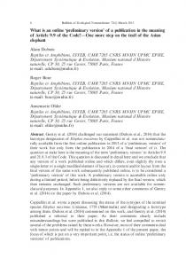
The experiments were done on KEGG/Ligand database version 49 (1.9.2008) containing a set of 7781 common biotransformation reactions. A total of 6015 reactions contained full and complete definition of the biotransformation. Rest of the reactions had missing, erroneous, ambiguous or unbalanced reaction definitions. These valid reactions were mapped using four algorithms: A*, maximum common subgraph (MCS) algorithm used by Hattori et al. (2003a) (with iteration cutoff parameter R = 100, 000), Bi-partite graph matching algorithm (implementation by Hungarian algorithm (Munkres, 1957; Riesen et al., 2007)) and naive greedy algorithm. All algorithms were implemented using Java and computed with 4 Gb of memory and Intel Xeon X5355 cpu running at 2.66 GHz. The A∗ algorithm managed to compute 5802 reactions, and our MCS implementation 5934 reactions, of the 6015 valid KEGG reactions in less than one hour per reaction. BPM and greedy algorithms computed all reactions. A total of 5624 reactions were computed with all algorithms and are comparable. As the A* algorithm finds an optimal atom mapping with respect to the edit distance, the main result is to compare how often MCS-based approach errs from this on real biochemical reactions represented by KEGG. We also analyze the performance of greedy and BPM procedures, and RPAIR pairwise mappings with respect to their edit distances. Figure 4 shows the count of reactions with respect to their difference from optimal edit distance. MCS algorithm optimally maps 5119 (91.0%) reactions. The difference is +2 for 359 reactions (6.4%), +4 for 66 (1.2%) and larger for 80 (1.4%) reactions. The two procedures suggested as pruning algorithms are of comparable accuracy. BPM and greedy algorithms achieve 63.3% and 54.4% optimal accuracy, 16

5500 MCS BPM Greedy

5000 4500 4000

Reaction count

3500 3000 2500 2000 1500 1000 500 0 0

2

4

6

8

10

12

14

16

18

20

22

24

26

28

30

Edit distance from optimal

Figure 4: Count of reactions with edit distance difference from optimal.

respectively. They differ from MCS by having a longer and wider tail. Both procedures are highly dependent on the performance of the similarity function and atom features. Both algorithms work well as pruning procedures where they are used numerous times during the A∗ search. Figure 5 shows the performance of the four algorithms. The reaction mappings are sorted by edit distance individually for each algorithm. The greedy and BPM algorithm’s results rise fast, while the MCS algorithm is effective for the majority of the reactions. The MCS also has a high tail indicating mappings where MCS procedure gives results of high edit distance. The MCS fails especially on reactions with high minimum edit distance. These reactions are often large and have complex reaction mechanism. The running times of A∗ and MCS algorithms are comparable (Figure not shown). Both algorithms suffer from high memory requirements, but in the A∗ algorithm smart pruning strategies can alleviate the problem. Also, because A∗ maintains both lower and upper bounds on the optimal solutions, insight into the optimality of the result achieved after early termination is acquired. KEGG RPAIR database contains a total of 10124 reactant-product mappings. We reconstructed reaction level mappings by combining the pairwise mappings of all reactant-product pairs of each reaction. Most of the reconstructed mappings only partially cover the reactants and products, or are not bijective. A total of 6851 reactions mappings can be at least partially reconstructed and 4364 of those are complete mappings. However, RPAIR entries use internal molecular definitions which differ from the standard definitions used in KEGG LIGAND. We couldn’t automatically match these two sources of molecular definitions, and hence only 2161 of the reconstructed mappings are consistent with KEGG LIGAND. These mappings are generated with SIMCOMP

17

50

50 A* MCS BPM Greedy

Edit distance

45

45

40

40

35

35

30

30

25

25

20

20

15

15

10

10

5

5

0

0 0

1000

2000

3000 Reactions

4000

5000

6000

Figure 5: Performance distributions of the four algorithms.

MCS algorithm and are manually curated (Kotera et al., 2004). 1932 of these mappings have the optimal edit distance, while only 16 are nonoptimal (all differing by 2). This is due to the manual curation of KEGG RPAIR. When these 2161 mappings are compared against the direct MCS mappings, 13 % of the reconstructed mappings have different edit distance compared to direct MCS mappings, signifying manual curation. 3% of the curated mappings have larger edit distance than uncurated mappings, while 97% have smaller edit distance. This indicates that domain experts almost always prefer the mappings with low edit distances.

5

Discussion and future work

Little is known about the process of enzymatic reactions with respect to the resulting atom mapping. In general the enzyme doesn’t need to minimize the edit distance – or to maximize the size of common subgraphs. The reaction mechanism is the result of chemical and physical interactions and laws, which in turn produce the atom mapping pattern. An interesting approximation of more realistic cost function is to use bond dissociation energies (Blanskby and Ellison, 2003), approximated with e.g. group contribution theory (Mavrovouniotis, 1991). An example of a reaction which does more work than needed is R00652 methionine:glyoxylate aminotransferase (see Figure 6). Here, the real transformation is thought to happen as shown on top (Glover et al., 1988), which requires a total of four operations: two cuts and two new bond formations. This 18

O

CH3

HO

MCS cost = 4

HO

NH2

O

O

O S

S HO

CH3

HO

O

O

NH2

R00652

O

O

O

S CH3

HO NH2

A* cost = 2

HO

O S

HO

CH3 O

O

HO NH2

Figure 6: Competing atom mappings of methionine:glyoxylate aminotransferase reaction. The MCS algorithm results in mapping of cost 4, while A∗ achieves a mapping of cost 2. However, the MCS mapping exhibits the correct reaction mechanism according to biochemical knowledge.

is the mapping the MCS algorithm finds. The A∗ algorithm finds the mapping shown on bottom, which includes only two operations. Here, the simpler mapping is unrealistic probably because of the high cost of cutting the methionine at the middle. In the MCS mapping only easily modifiable oxygen and nitrogen atoms are operated at the edges of the molecules. The A∗ cost function could be extended to take this into account. Enzymes catalyzing reactions can be classified into groups such as transferases or isomerases according to e.g. enzyme classification (EC) system. This contextual information could be used to infer the type of reaction and the likely type of transformation of the reaction. The structural information of the enzymes and substrates of a reaction could be used for 3D modeling and prediction of the likely site-of-modification. 3D modeling has been actively researched in drug design (de Graaf et al., 2005). An interesting development to the framework presented here would be to explicitly model the symmetry classes of optimal atom mappings. That is, all mappings which are automorphic. As seen in Figure 3, symmetrical atoms lead to duplication of the number of optimal mappings. Handling of automorphic mappings can be either designed into an mapping algorithm or be done afterwards to classify the resulting mappings into symmetry classes. We have implemented an VF2-based isomorphism algorithm which can answer whether two bi-graph mappings (i.e. atom mappings) are isomorphic (Cordella et al., 1999, 2004). To our knowledge, no current method deals with symmetries directly in the mapping algorithm itself. In a setting where only one optimal mapping is sufficient, the upper bound can be optimized. Instead of setting the upper bound to the cost of current best 19

mapping, it can be set to f (M ) − 1 as we are only interested in mappings which are better than the current best mapping. This leads to more effective pruning of the search space. This strategy is especially effective as the cost function f is discrete and often small (see Figure 5).

6

Conclusions

This article describes a novel A∗ algorithm for atom mapping problem. The proposed method isn’t based on the the maximum common substructures, but utilizes a sophisticated cost function to determine the atom mapping which incurs the minimum number of edge operations. The algorithm uses smart heuristics to guide itself through the space of atom mappings and guarantees an optimal result. The A∗ algorithm is well-defined and can be modified to use any cost function to determine a good atom mapping. We also propose a novel set of atom features, which are used to distinguish between similar atoms. The algorithm was used against KEGG database and the resulting mappings agree well with the RPAIR database mappings, which are manually curated.

Author contributions MH, TM and JR designed the algorithms. SL and MH implemented the algorithms. MH conducted the experiments. JR and MH designed the experiments and co-wrote the manuscript.

Acknowledgements This work was supported by Academy of Finland grant 118653 (ALGODAN) and in part by the IST Programme of the European Community under PASCAL2 Network of Excellence, IST-2007-216886. This publication only reflects the authors’ views.

References T. Akutsu. Efficient extraction of mapping rules of atoms from enzymatic reaction data. J. Computational Biology, 11:449–462, 2004. M. Arita. Graph modeling of metabolism. Journal of Japan Society of Artificial Intelligence, 15:703–710, 2000. M. Arita. In silico atomic tracing by substrate-product relationships in escherichia coli intermediary metabolism. Genome Res., 13:2455–2466, 2003. M. Arita. Introduction to the arm database: Database on chemical transformation in metabolism for tracing pathways. In Metabolomics, The Frontier of Systems Biology, volume 4, pages 193–210. Springer Tokyo, 2005.

20

K. Astikainen, E. Pitk¨ anen, and J. Rousu. Structured output prediction approaches for novel enzyme function. In First international conference on Bioinformatics, Valencia, Spain, January, page to appear, 2010. S Bereg. Topological indices in combinatorial chemistry. In Bioinformatics Algorithms: Techniques and Applications, pages 419–463. John Wiley & Sons, Inc., 2008. S. Blanskby and G. Ellison. Bond dissociation energies of organic molecules. Acc. Chem. Res, 36:255–263, 2003. T. Blum and O. Kohlbacher. Using atom mapping rules for an improved detection of relevant routes in weighted metabolic networks. J. Computational Biology, 15:565–576, 2008. C. Bron and J. Kerbosch. Finding all cliques of an undirected graph. Communications of the ACM, 16:575–577, 1971. H. Bunke. Graph matching: Theoretical foundations, algorithms, and applications. In Proc. Vision Interface, pages 82–88, 2000. F. Cazals and C. Karande. An algorithm for reporting maximal c-cliques. Theoretical Computer Science, 349:484–490, 2005. F. Cazals and C. Karande. A note on the problem of reporting maximal cliques. Theoretical Computer Science, 407:564–568, 2008. M. Cone, R. Venkataraghaven, and F. McLafferty. Molecular structure comparison program for the identification of maximal common substructures. J. Am. Chem. Soc., 99:7668–7671, 1977. L. Cordella, P. Foggia, C. Sansone, and M. Vento. A (sub)graph isomoprhism algorithm for matching large graphs. IEEE Transactions on Pattern Analysis and Machine Intelligence, 26:1367–1372, 2004. L. P. Cordella, P. Foggia, C. Sansone, and M. Vento. Performance evaluation of the vf graph matching algorithm. In ICIAP ’99: Proceedings of the 10th International Conference on Image Analysis and Processing, page 1172. IEEE Computer Society, 1999. J.D. Crabtree and D.P. Mehta. Automatic reaction mapping. ACM Journal of Experimental Algorithms, 13, 2009. C. de Graaf, N.P.E. Vermeulen, and K.A. Feenstra. Cytochrome p450 in silico: An integrative modeling approach. Journal of Medicinal Chemistry, 48:2725– 2755, 2005. R. Dechter and J. Pearl. Generalized best-first search strategies and the optimality of a∗ . Journal of the ACM, 32:505–536, 1985.

21

N.C. Duarte, S.A. Becker, N. Jamshidi, I. Thiele, M.L. Mo, T.D. Vo, R. Srivas, and B.O. Palsson. Global reconstruction of the human metabolic network based on genomic and bibliomic data. Proceecings of the National Academy of Sciences, 104, 2007. J. Gao, S. Ma, D.T. Major, K. Nam, J. Pu, and D.G. Truhlar. Mechanisms and free energies of enzymatic reactions. Chem. Rev., 106:3188–3209, 2006. J.R. Glover, C.C.S. Chapple, S. Rothwell, I. Tober, and B.E. Ellis. Allylglucosinolate biosynthesis in brassica carinata. Phytochemistry, 27:1345–1348, 1988. S. Goto, Y. Okuno, M. Hattori, Nishioka T., and Kanehisa M. LIGAND: A database of chemical compounds and reactions in biological pathways. Nucleic Acids Research, 30:402–404, 2002. P.E. Hart, N.J. Nilsson, and B. Raphael. A formal basis for the heuristic determination of minimum cost paths. IEEE Transactions on Systems Science and Cybernetics, 4:100–107, 1968. M. Hattori, Y. Okuno, S. Goto, and M. Kanehisa. Heuristics for chemical compound matching. Genome Inform., 14:144–153, 2003a. M. Hattori, Y. Okuno, S. Goto, and M. Kanehisa. Development of a chemical structure comparison method for integrated analysis of chemical and genomic information in the metabolic pathways. J. American Chemical Society, 125: 11853–65, 2003b. T. Hogiri, C. Furusawa, Y. Shinfuku, N. Ono, and H. Shimizu. Analysis of metabolic network based on conservation of molecular structure. BioSystems, 95:175–178, 2008. M. Kanehisa and S. Goto. KEGG: Kyoto Encyclopedia of Genes and Genomes. Nucleic Acids Research, 28:27–30, 2000. M. Kanehisa, S. Goto, M. Hattori, K. Aoki-Kinoshita, M. Itoh, S. Kawashima, T. Katayama, M. Araki, and M. Hirakawa. From genomics to chemical genomics: new developments in kegg. Nuclead Acids Research, 34:354–357, 2006. P. D. Karp, M. Arnaud, J. Collado-Vides, J. Ingraham, I. T. Paulsen, and M. H. Saier Jr. The E. coli EcoCyc Database: No Longer Just a Metabolic Pathway Database. ASM News, 70(1):25–30, 2004. Douglas Kell. Metabolomics and systems biology: Making sense of the soup. Current Opinion in Microbiology, 7:296–307, 2004. H. Kitano. Systems biology: A brief overview. Science, 295:1662–1664, 2002. I. Koch. Enumerating all connected maximal common subgraphs in two graphs. Theoretical Computer Science, 250:1–30, 2001. 22

M. Kotera, M. Hattori, M-A. Oh, R. Yamamoto, T. Komeno, J. Yabuzaki, K. Tonomura, S. Goto, and M. Kanehisa. Rpair: a reactant-pair database representing chemical changes in enzymatic reactions. Genome Inform., 15: P062, 2004. G. Levi. A note on the derivation of maximal common subgraphs of two directed or undirected graphs. Calcolo, 9:1–12, 1972. M. Lynch. Storage and retrieval of information on chemical structures by computer. Endeavour, 27:68–73, 1968. M. Lynch and P. Willett. The automatic detection of chemical reaction sites. J. Chem. Inf. Comp. Sci., 18, 1978. M. Mavrovouniotis. Estimation of standard gibbs energy changes of biotransformations. Journal of Biological Chemistry, 266:14440–14445, 1991. J. McGregor and P. Willett. Use of a maximal common subgraph algorithm in the automatic identification of the ostensible bond changes occurring in chemical reactions. J. Chem. Inf. Comp. Sci., 21, 1981. B. Menk¨ uc, C. Gille, and H. Holzh¨ utter. Computer aided optimization of carbon atom labeling for tracer experiments. Genome Inform., 20:270–276, 2008. F. Mu, R. Williams, C. Unkefer, P. Unkefer, J. Faeder, and W. Hlavacek. Carbon-fate maps for metabolic reactions. Bioinformatics, 23:3193–3199, 2007. J. Munkres. Algorithms for the assignment and transporation problems. J. Society for Industrial and Applied Mathematics, 5:32–38, 1957. E. Pitk¨ anen, A. Rantanen, J. Rousu, H. Maaheimo, and E. Ukkonen. A computational method for reconstructing gapless metabolic networks. In Bioinformatics Research and Development, Communications in Computer and Information Science, pages 288–302. Springer, 2008. E. Pitk¨ anen, P. Jouhten, and J. Rousu. Inferring branching pathways in genome scale metabolic networks. BMC Systems Biology, 3, 2009. E. Pitk¨ anen, J. Rousu, and E. Ukkonen. Computational methods for metabolic reconstruction. Current Opinion in Biotechnology, page to appear, 2010. A. Rantanen, T. Mielik¨ ainen, J. Rousu, H. Maaheimo, and E. Ukkonen. Planning optimal measurements of isotopomer distributions for estimation of metabolic fluxes. Bioinformatics, 22:1198–1206, 2006. A. Rantanen, J. Rousu, P. Jouhten, N. Zamboni, H. Maaheimo, and E. Ukkonen. An analytic and systematic framework for estimating metabolic flux ratios from 13c tracer experiments. BMC Bioinformatics, 9:266–285, 2008.

23

J. Raymond and P. Willett. Maximum common subgraph isomorphism algorithms for the matching of chemical structures. J. Computer-Aided Molecular Design, 16:521–533, 2002. K. Riesen, M. Neuhaus, and H. Bunke. Bipartite graph matching for computing the edit distance of graphs. Graph-Based Representations in Pattern Recognition, pages 1–12, 2007. J. Rousu, A. Rantanen, H. Maaheimo, E. Pitk¨anen, K. Saarela, and E. Ukkonen. A method for estimating metabolic fluxes from incomplete isotopomer information. In Computational Methods in Systems Biology, volume 2602 of Lecture Notes in Computer Science, pages 88–103. Springer, 2003. E. Sussenguth. A graph-theoretical algorithm for matching chemical structures. J. Chem. Doc., 5:36–43, 1965. R. Tarjan. Graph algorithms in chemical computation. In R. Christofferson, editor, Algorithms for Chemical Computations, pages 1–20. American Chemical Society, 1977. R. Uehara, S. Toda, and T. Nagoya. Graph isomorphism completeness for chordal bipartite graphs and strongly chordal graphs. Discrete Applied Mathematics, 145:479–482, 2005. T. Wang and J. Zhou. Emcss: A new method for maximal common substructure search. J. Chem. Inf. Comp. Sci., 37:828–834, 1997. W. Wipke and T. Dyott. Stereochemically unique naming algorithm. Journal of American Chemical Society, 96:4834–4842, 1974. J. Xu. Gma: A generic match algorithm for structural homomorphism, isomorhism, and maximal common substructure match and its applications. J. Chem. Inf. Comp. Sci., 36:25–34, 1996. Y. Yamanishi, M. Hattori, M. Kotera, S. Goto, and M. Kanehisa. E-zyme: predicting potential ec numbers from the chemical transformation pattern of substrate-product pairs. Bioinformatics, 25:179–186, 2009.

24