Geosci. Model Dev., 4, 419–433, 2011 www.geosci-model-dev.net/4/419/2011/ doi:10.5194/gmd-4-419-2011 © Author(s) 2011. CC Attribution 3.0 License.
Geoscientific Model Development
PREP-CHEM-SRC – 1.0: a preprocessor of trace gas and aerosol emission fields for regional and global atmospheric chemistry models S. R. Freitas1 , K. M. Longo2 , M. F. Alonso1 , M. Pirre3 , V. Marecal4 , G. Grell5 , R. Stockler1 , R. F. Mello1 , and M. S´anchez G´acita1 1 Center
for Weather Forecasting and Climate Studies, INPE, Cachoeira Paulista, Brazil System Science Center, INPE, S˜ao Jos´e dos Campos, Brazil 3 Laboratoire de Physique et Chimie de l’Environnement et de l’Espace, CNRS-Universit´ e d’Orl´eans, Orl´eans, France 4 Centre National de Recherches M´ et´eorologique/Groupe d’´etude de l’Atmosph`ere M´et´eorologique, M´et´eo-France and CNRS, Toulouse, France 5 Cooperative Institute for Research in Environmental Sciences (CIRES) and NOAA Earth Systems Research Laboratory (ESRL), USA
2 Earth
Received: 24 May 2010 – Published in Geosci. Model Dev. Discuss.: 23 June 2010 Revised: 12 April 2011 – Accepted: 5 May 2011 – Published: 10 May 2011
Abstract. The preprocessor PREP-CHEM-SRC presented in the paper is a comprehensive tool aiming at preparing emission fields of trace gases and aerosols for use in atmosphericchemistry transport models. The considered emissions are from the most recent databases of urban/industrial, biogenic, biomass burning, volcanic, biofuel use and burning from agricultural waste sources. For biomass burning, emissions can be also estimated directly from satellite fire detections using a fire emission model included in the tool. The preprocessor provides emission fields interpolated onto the transport model grid. Several map projections can be chosen. The inclusion of these emissions in transport models is also presented. The preprocessor is coded using Fortran90 and C and is driven by a namelist allowing the user to choose the type of emissions and the databases.
1
Introduction
Atmospheric chemistry composition studies with numerical simulations are widely conducted due to the increasing availability of atmospheric-chemistry transport models and computational resources. Emission inventories of trace gases and aerosols provide surface as well as upper level mass fluxes Correspondence to: S. R. Freitas (
[email protected])
for the mass continuity equation (MCE), which are crucial needed information for these numerical studies. To provide this information, several international programs and groups have been developing emission inventories of the most relevant primary atmospheric trace gases and aerosols. For example, we can cite the Global Fire Emissions Database (GFED, van der Werf et al., 2006) for biomass burning and the “REanalysis of the TROpospheric chemical composition over the past 40 yr” (RETRO, http://retro.enes.org) for urban emissions. The numerical simulation of atmospheric chemistry composition is done with advanced models where the MCE is solved on- or off-line (Zhang, 2008) with several spatial resolutions and geographical projections, on either regional or global scales. In this paper, we introduce a software tool, named PREP-CHEM-SRC, version 1.0, developed to provide gridded emissions of trace gases and aerosols with a flexible spatial resolution, several projections and suitable for regional and global models. Emission fields generated by this system have been used with CCATT-BRAMS (Freitas et al., 2009, Longo et al., 2011), WRF-CHEM (Grell et al., 2005), and the Flow-following finite-volume Icosahedral Model (FIM, Bleck et al., 2010). The emission preprocessor was also implemented for use with the Brazilian Center for Weather Forecasting and Climate Studies (CPTEC) global circulation model. This paper is organized as follows. Section 2 covers all available inventories of emissions from anthropogenic and biogenic sources as well as the chemical species available in
Published by Copernicus Publications on behalf of the European Geosciences Union.
420
S. R. Freitas et al.: PREP-CHEM-SRC – 1.0
the database of this software tool. In Sect. 3, we briefly describe a possible way to introduce the emission contribution in the MCE. Section 4 describes the system and its functionalities. Our conclusions are discussed in Sect. 5.
2
Emission inventories
This section is devoted to describe all types of emissions currently available within the PREP-CHEM-SRC system. This covers emissions of gases and aerosols from urban/industrial, biogenic, biomass burning, volcanic sources and from biofuel use and burning of agricultural waste. For urban/industrial and biogenic emissions from several databases are available and may be chosen by the user. For biomass burning, it is possible to use the Global Fire Emissions Database with a 8 days or a one month resolution or the Brazilian biomass burning emission model tool (Longo et al., 2010). This model provides emissions with very high temporal and spatial resolutions from satellite fire detection. Volcanic emissions include ashes for erupting periods and SO2 degassing for both eruptive and non-eruptive periods. Depending on the modeling system the user may select all emission options (anthropogenic, biogenic, biomass burning, etc) or select only part of the entire available set. WRFCHEM, for example, has several other emission preprocessors, depending on the location of the domain in which the model will be run. The user may choose to combine his or her own anthropogenic emission preprocessor with only the biomass burning emissions from our system. 2.1
Urban-industrial emissions
For the urban/industrial emissions, three alternative emission datasets are available, which include different time horizons, resolutions and set of species. One of the anthropogenic emission inventories used within the PREP-CHEM-SRC system is provided by the “REanalysis of the TROpospheric chemical composition over the past 40 yr” (RETRO, http://retro.enes.org), a long-term global modeling study of tropospheric chemistry funded by the 5th European Commission Framework Programme. The emission data has a 0.5◦ × 0.5◦ spatial resolution and global coverage, with monthly temporal resolution, and is based on the year 2000. The emission units are kg [species] m−2 dy−1 . The Table 1 provides a list of chemical species available in the anthropogenic inventory. The second database proposed for anthropogenic emissions is provided by the “Emission Database for Global Atmospheric Research” (EDGAR, http://edgar.jrc.ec.europa. eu, Olivier et al., 1996, 1999). This program provides past and present global anthropogenic emissions of greenhouse gases and air pollutants. The available species are N2 O, CO2 , CO, CH4 , SO2 , SF6, NOx and NMVOC with a 1◦ × 1◦ spatial resolution. The emissions do not vary in time and are Geosci. Model Dev., 4, 419–433, 2011
based on the year 2000. A recently released new version of EDGAR, version 4, will be included in the database of the PREP-CHEM-SRC system in an upcoming version. Additionally, for the South American continent, a regional urban emission inventory suitable either for local and regional scale applications is also available. This database integrates information from local vehicle emission inventories using socio-economic data, extrapolation of emissions for cities lacking local inventories, and the geographic distribution of emissions at different spatial resolutions (Alonso et al., 2010). For aerosols, emissions of organic carbon (OC), black carbon (BC), SO2 and DMS at a 1◦ × 1◦ resolution on a monthly basis from the Goddard Chemistry Aerosol Radiation and Transport (GOCART) model database are provided. 2.2 2.2.1
Biogenic emissions Biogenic emissions from GEIA Activity
The first database proposed for biogenic or natural emissions is the GEIA/ACCENT Activity on Emission Databases, http://www.aero.jussieu.fr/projet/ACCENT/ description.php). Emission sources from land, vegetation and oceans are provided with a 1◦ × 1◦ spatial resolution and monthly temporal resolution. Emissions for Acetone, C2 H4 , C2 H6 , C3 H6 , C3 H8 , CO, CH3 OH, DMS, NO, Isoprene, Terpenes and NVOC are available. The emission units are kg [species] m−2 dy−1 . 2.2.2
Biogenic emissions from MEGAN
The alternative biogenic emission database is derived by the Model of Emissions of Gases and Aerosols from Nature (MEGAN, Guenther et al., 2006). MEGAN is a modeling system for estimating the net emission of gases and aerosols from terrestrial ecosystems into the atmosphere. Driving variables used by MEGAN to calculate the fluxes include land cover, weather, and atmospheric chemical composition. The data was provided by the GEIA/ACCENT Activity on Emission Databases, http://www.aero.jussieu.fr/ projet/ACCENT/description.php. The data covers the entire world with a 0.5◦ × 0.5◦ spatial resolution. The temporal coverage is from January to December 2002 with a monthly time resolution. Emission rates are provided for the following species: CO, CH4 , C2 H4 , C2 H6 , C3 H6 , C3 H8 , CH3 OH, Formaldehyde, Acetaldehyde, Acetone, other Ketones, Toluene, Isoprene, Monoterpenes and Sesquiterpenes. The emission units are kg [species] m−2 dy−1 . 2.3
Biomass burning emissions and the smoke plume rise model
Emissions from wild- or deforestation fires are provided using two methodologies.
www.geosci-model-dev.net/4/419/2011/
S. R. Freitas et al.: PREP-CHEM-SRC – 1.0
421
Table 1. List of chemical species available in the anthropogenic inventory developed by the RETRO program.
2.3.1
Acids
C4 H10
Ethene
Alcohols
C5 H12
Ethers
Other VOC
Benzene
C6 H14 plus higher alkanes
Ethyne
Toluene
C2 H2
Chlorinated Hydrocarbons
Ketones
Trimethylbenzene
C2 H4
CO
Methanal
Xylene
C2 H6
Esters
NOx
C3 H8
Ethane
Other Alkanals
Brazilian biomass burning emission model
The first option is based on the Brazilian Biomass Burning Emission Model (3BEM, Longo et al., 2010) which is included in this software tool. In this methodology, for each fire pixel detected by remote sensing, the mass of the emitted tracer is calculated by the following expression, which takes into consideration the estimated values for the amount of above-ground biomass available for burning (α), the combustion factor (β), the emission factor (EF) for a certain species (η) from the appropriate vegetation type, and the burning area (afire ) for each burning event. M [η] = αveg · βveg · EF[η] veg · afire
(1)
In this model, a hybrid remote-sensing fire product is used to minimize missing remote sensing observations. The fire database actually used is a combination of the Geostationary Operational Environmental Satellite – Wildfire Automated Biomass Burning Algorithm (GOES WF ABBA) product (cimss.ssec.wisc.edu/goes/burn/wfabba.html; Prins et al., 1998), the Brazilian National Institute for Space Research (INPE) fire product, which is based on the Advanced Very High Resolution Radiometer (AVHRR) aboard the NOAA polar orbiting satellites series (www.cptec.inpe. br/queimadas; Setzer and Pereira, 1987), and the Moderate Resolution Imaging Spectroradiometer (MODIS) fire product (modis-fire.umd.edu; Giglio et al., 2003). The three fire product databases are combined using a filter algorithm to avoid double counting of the same fire, by eliminating additional fires within a circle with a radius of 1 km. The burnt area of fires detected in the GOES WF ABBA product is estimated from the instantaneous fire size for each non-saturated and non-cloudy fire pixel, from which it is possible to retrieve sub-pixel fire characteristics. For GOES WF ABBA detected fires that have no information about the instantaneous fire size, a mean instantaneous fire size of 0.14 km2 (calculated from the GOES ABBA database of the previous years) is used. For fires detected by the MODIS and AVHRR systems, a mean value of 0.22 km2 of burnt area is used (Longo et al., 2010). The fire detection maps with latitude and longitude are merged with 1 km resolution land cover data (Belward, 1996, www.geosci-model-dev.net/4/419/2011/
Other Aromatics
Sestini et al., 2003) to provide the associated emission (EF) and combustion (β) factors through a look-up table. The corresponding aboveground carbon density (α) is defined from the carbon in live vegetation data, estimated using Olson et al. (2000) and updated by Gibbs (2006) and Gibbs et al. (2007) using the Global Land Cover Database (GLC2000). For the Amazon basin and neighboring areas, the estimation of aboveground carbon density done by Saatchi et al. (2007) with 1 km spatial resolution is used. The land cover map for the Amazon basin was updated with data provided by the PROVEG project (Sestini et al., 2003) and it is based on the year 2000. The emission and combustion factors for each biome are based on Andreae and Merlet (2001) and Longo et al. (2009). In particular, Andreae and Merlet (2001) provides emission factors for 110 chemical species emitted during burning of tropical forest, extratropical forest, savanna, pasture, charcoal production andagricultural waste, as well as emission factors measured in controlled laboratory experiments. The mean combustion factor for each biome cited above is also provided. See Table 2 for a complete list of species available within the PREP-CHEM-SRC system. The total emitted mass of each chemical species per grid box is calculated by summing the individual mass (given by Eq. 1) over all fires in that grid box. The emission units are kg [species] m−2 dy−1 . 2.3.2
The Global Fire Emissions Database
The second methodology available for biomass burning emissions is based on Giglio et al. (2006) and van der Werf et al. (2006). These authors use burnt-area estimates from remote sensing, a biogeochemical model, and emission factors from the literature to estimate fire emissions during the 8yr period from 1997 to 2004. This dataset, called the Global Fire Emissions Database (GFEDv2), has a 1◦ ×1◦ spatial resolution and a 8-day or one-month temporal resolution. In this case, the GFEDv2 emissions are interpolated to the model grid and the same list of species described in the Table 2 is available. The emission units are kg [species] m−2 dy−1 . Figure 1 illustrates the typical output of the PREP-CHEMSRC system for biomass burning. It shows the spatial Geosci. Model Dev., 4, 419–433, 2011
422
S. R. Freitas et al.: PREP-CHEM-SRC – 1.0
Table 2. List of species available within the PREP-CHEM-SRC system for biomass burning emissions. CO2
n butane
n hexane
Butanols
CO
i-butane
isohexanes
cyclopentanol
CH4
1 pentene
heptane
phenol
NHMC
2 pentene
octenes
Formaldehyde
C2 H2
n pentane
terpenes
Acetald
C2 H4
2 Me Butene
benzene
Hydroxyacetaldehyde
C2 H6
2 Me butane
toluene
Acrolein
C3 H4
pentadienes
xylenes
Propanal
C3 H6
Isoprene
ethylbenzene
Butanals
C3 H8
cyclopentene
styrene
Hexanals
1 butene
cyclopentadiene
PAH (polycyclic aromatichydrocarbons )
Heptanals
i-butene
4 me 1 pentene
Methanol
Acetone
tr 2 butene
2 me 1 pentene
Ethanol
2 Butanone
cis 2 butene
1 hexene
1 Propanol
2 3 Butanedione
butadiene
hexadienes
2 propanol
Pentanones
Hexanones
Acrylonitrile
NH3
Heptanones
Heptanones
Propionitrile
HCN
Octanones
Octanones
pyrrole
cyanogen
Benzaldehyde
Benzaldehyde
trimethylpyrazole
SO2
Furan
Furan
methylamine
DMS
H2
2 Me Furan
dimethylamine
COS
NOx
3 Me Furan
ethylamine
CH3 Cl
NOy
2 ethylfuran
trimethylamine
CH3 Br
N2 O
2 4 dime furan
n pentylamine
CH3 I
benzofuran
2 5 Dime furan
2 me 1 butylamine
Hg
Propanoic
Tetrahydrofuran
PM2.5 (particulate matter 1 (above) where 1z1 is the vertical thickness of the first physical model layer where the tracer η will be released and k denotes the vertical layer. If the emission source is located above the first model vertical layer, as would be the case for tall chimneys with a height greater than the thickness of this layer, Eq. (4) must be changed accordingly. The unit of the emission rate E¯ η in Eq. (4) is kg [η] (kg [air] dy)−1 . To express the emission rate per second instead of per day, the user has two choices. If the diurnal cycle of the process that is emitting the tracer is constant, Eq. (4) must be divided by 86 400 s dy−1 . However, several processes release tracers at non-homogenous rates during the day. Consequently, the user should develop a diurnal cycle function r(t) which obeys the following constraint Z 86400 r(t)dt = 1, (5) 0
Geosci. Model Dev., 4, 419–433, 2011
Fig. 2. A double Gaussian function used to determine the diurnal cycle of urban emission.
In this case, the instantaneous emission rate will be given by ( F η r(t), k = 1 (surface) ¯ 1 ) 1z1 E¯ η (k,t) = ρ(k , (6) 0, k > 1 (above) with units of kg [η] (kg [air] s)−1 . For emissions from mobiles sources in urban areas, r(t) could, for example, be represented by a double Gaussian function with one peak in the morning and another one in the late afternoon, representing the typical rush hours in the cities, as illustrated in Fig. 2. In case of a constant daily emission, r(t) is simply given by 1/86400. 3.2
Hot/high buoyancy emissions
One important example of hot and high buoyancy emissions are those from vegetation fires. This process emits hot gases and particles which are quickly transported upward due the positive buoyancy produced by the combustion. The entire fire process can be split in two main phases: – smoldering with most of the emission released just above the surface, – flaming with most of the emission directed injected in the PBL, free troposphere or even stratosphere. In the methodology proposed by Freitas et al. (2006, 2007, 2010), a 1-D plume rise model is embedded in each column of the 3-D low resolution atmospheric chemistry-transport models (the hosts) to interactively provide the smoke injection height, the actual region where the trace gases and aerosols emitted during the flaming phase of vegetation fires are released in the atmosphere. Following this approach, the total emission flux (Fη , in units of kg [η] m−2 dy−1 ) is first determined, followed by www.geosci-model-dev.net/4/419/2011/
S. R. Freitas et al.: PREP-CHEM-SRC – 1.0
425
Fig. 3. (A)3. An(A) example a simulatedof vertical cross sectionvertical of biomass burning CO source on 18:00 UTC 02CO September 2002 Figure An ofexample a simulated cross section ofemission biomass burning source at latitude 5.4◦ S (adapted from Freitas et al., 2007). It shows the surface emission associated to the smoldering phase as well as elevated emission layers associated to the flaming The panel (B) depictsat a Gaussian function at 15:00 LT used toFreitas determineet theal., diurnal emission on 1800 UTC 02phase. September 2002 latitude 5.4 centered S (adapted from cycle of biomass burning emissions on South America.
2007). It shows the surface emission associated to the smoldering phase as well as elevated theemission partitioninglayers of massassociated emitted during reported by Prins al. (1998).a Figure 3b shows the diurnal to the thesmoldering flaming and phase.asThe panel (B)etdepicts Gaussian function flaming phases. Finally, the plume rise model determines the cycle function r(t) as used by the CCATT-BRAMS model. smoke injection of the flaming phase. Fromthe the above, For other tropical areas of the world, Giglio on (2007) reports centered at layer 15 LT used to determine diurnal cycle of biomass burning emissions South the emission term of Eq. (2) can be expressed as the diurnal fire cycles for 15 regions which can be used to America. describe the corresponding diurnal cycle functions r(t). ( Fη λ ,k = 1 ρ(k ¯ 1 ) 1z1 E¯ η (k) = (7) Fη 1zh 1zh (1 − λ) ρ(k) ¯ 1zk ,h − 2 < z(k) < h + 2 4 System description and functionalities where 1zh is thei vertical thickness of the smoke layer, h 4.1 Chemical mechanisms available, grid projection 1zh h − 2 , h + 1z2 h is the vertical domain of the injection and interpolation methods layer prescribed by the smoke plume rise model and λ is the PREP-CHEM-SRC is ready to provide emissions for the fraction (between 0 and 1) of the total mass released to the chemical mechanisms RADM2 (Chang et al., 1989), RACM atmosphere during the smoldering phase. An example of the (Stockwell et al., 1997), CB07 (Yarwood et al., 2005) and spatial distribution of biomass burning CO source emissions RELACS (Crassier et al., 2000). The chemical mechanism is given by Fig. 3a. It shows a vertical cross section of CO is determined during the code compilation by providing the emissions at 18:00 UTC on 2 September 2002 along latitude corresponding chem1 list.f90 file (see the README file for 5.4◦ S (see Freitas et al., 2007 for more details), with surfurther instructions). face emission associated with smoldering phase as well as Several options of map projection types (Polarelevated emission layers associated with flaming phase. Stereographic, Gaussian, Lambert Conformal, Rectangular, To convert the time unit of emission to seconds, it is conFIM model Icosahedral horizontal grid ) for regional and venient to introduce a diurnal cycle for the biomass burnglobal grids are available with flexible spatial resolution. ing emissions. The burning diurnal cycle typically shows The interpolation routines to create the emission fields on a peak between approximately 13:00 and 18:30 local time, the model grid box can use either nearest-neighbor interpolawith the fire activity peaking earlier for heavily forested retion (when the model grid spacing is finer than the database gions. The diurnal fire cycle is dictated primarily by the digrid spacing) or box averaging (when the model resolution urnal cycle of human activity; however, for high fractional is coarser). Both methods are approximately mass conservatree cover, the diurnal meteorological conditions limit ignitive. tion to a relatively brief period of the day (Giglio, 2007). For South American fires, a single Gaussian function centered at The code is modular, user friendly, and self-explanatory Figure 4. Carbon monoxide generated by the source PREP-CHEM-SRC ∼18:00 UTC is normally used. Thisanthropogenic curve is based onemission the on field how each kind of emission is treated. A regular typical diurnal cycle of fire occurrence over South America user should be able to easily include new emission databases,
program: Panel (A) for a regional grid with 15 km horizontal resolution, Panel (B) for a
nested grid with 3 km. The black www.geosci-model-dev.net/4/419/2011/ in the coarse domain.
box on Panel (A) represents theGeosci. location ofDev., the 4, nested grid Model 419–433, 2011
426
S. R. Freitas et al.: PREP-CHEM-SRC – 1.0
Fig. 4. Carbon monoxide anthropogenic emission field generated by the PREP-CHEM-SRC program: Panel (A) for a regional grid with 15 km horizontal resolution, Panel (B) for a nested grid with 3 km. The black box on Panel (A) represents the location of the nested grid in the coarse domain.
such as aircraft emissions, for example. Feedback to the developers is welcome. 4.2
The software
The PREP-CHEM-SRC emissions tool is coded using Fortran90 and C and requires HDF and NetCDF libraries. The code package is comprised of Fortran90 and C routines and a README file for further instructions. We make intensive use of derived type data and modules, functionalities of Fortran90, to provide clear, safe and easy understanding of the data structure. The desired grid configuration and emission inventories to provide trace gases and aerosol fluxes are defined in a Fortran namelist file called “prep-chem-src.inp”. The Appendix A provides a description of the parameters in the namelist. The software has been tested with Intel and Portland Fortran compilers under the UNIX/LINUX operating system. 4.3
Some examples of regional and global emissions
For regional models with nested grid capability, emissions for both coarse and fine grids are provided. Local updates for megacities or inclusion of point and line sources can easily be implemented. The product of this tool is a set of files with gridded daily emission fluxes (kg m−2 dy−1 ) and emission related information fields. Figure 4 introduces the first example of the model output. In this case it is related to the anthropogenic emission of CO (described at Sect. 2.1) in the southeast region of Brazil. The system was configured with 2 grids, the coarse one (showed in panel a) with a 15 km horizontal resolution Geosci. Model Dev., 4, 419–433, 2011
covering mostly of S˜ao Paulo State with Paran´a State in the south and Rio de Janeiro and Minas Gerais states in the north. The second and nested grid (panel b) has a 3 km horizontal resolution and covers the more densely urbanized areas of the Brazil, S˜ao Paulo and Rio de Janeiro Metropolitan Areas (MA), indicated by the letters SP and RJ on the panel. At this resolution, the shape of the emission field resembles much better the real urban islands of these Metropolitan Areas. Another remarkable feature at this resolution is the emission related to the main highways and roads of this area depicted by the red lines connecting SP and RJ and others urbanized locations. See Alonso et al. (2010) for more details. As an example of model output for a regional grid covering South America, Figs. 5 and 6 show SO2 and NO emission estimates for a specific day, respectively. Figure 5 shows sources of SO2 estimated for 27 August 2002 on a rectangular projection grid with a spatial resolution of 0.2◦ × 0.2◦ . Panel a shows volcanic SO2 emissions (in units 10−9 kg m−2 dy−1 , see Sect. 2.4) along the Andes Mountains on the east side of South America. Panel b shows the emission associated with biomass burning as estimated using the 3BEM methodology; in this case fire counts from MODIS and the WF ABBA fire product were used (Sect. 2.3). Finally, Panel (c) illustrates the SO2 emissions from urban and industrial processes as prescribed by the EDGAR inventory (Sect. 2.1). For NO, Fig. 6 shows the biogenic emission (A) from GEIA (Sect. 2.2), from biomass burning (B) from 3BEM (Sect. 2.3) and anthropogenic (C) from RETRO revised with local sources of information according to Alonso et al. (2010, Sect. 2.1).
www.geosci-model-dev.net/4/419/2011/
S. R. Freitas et al.: PREP-CHEM-SRC – 1.0
427
Fig. 5. Different sources of SO2 estimated for 27 August 2002 on a rectangular projection grid with spatial resolution of 0.2◦ × 0.2◦ . Panel (A) represents volcanic emission following Diehl, 2009 inventory, (B) biomass burning from 3BEM and (C) anthropogenic SO2 using EDGAR.
Fig. 6. Different sources of NO estimated for 27 August 2002 on a rectangular projection grid with spatial resolution of 0.2◦ ×0.2◦ . Panel (A) represents biogenic emission following GEIA inventory, (B) biomass burning NO emission from 3BEM and (C) anthropogenic NO using RETRO data but updated with local sources of information for the South American main cities.
www.geosci-model-dev.net/4/419/2011/
Geosci. Model Dev., 4, 419–433, 2011
428
S. R. Freitas et al.: PREP-CHEM-SRC – 1.0
Fig. 7. Carbon monoxide emission field generated by the PREP-CHEM-SRC program for the icosahedral grid (level G5, resolution around 250 km) of FIM Model.
Emissions processed on the global scale for the FIM global model icosahedral grid is shown in Fig. 7. In this case, anthropogenic (Sect. 2.1) and biomass burning emissions (Sect. 2.3, using the MODIS fire product) of carbon monoxide are processed on a G5 grid resolution, approximately 250 km. Most emissions displayed in the left panel of Fig. 7 are associated with dense industrial and urban areas. On the right, urban emissions over Europe and biomass burning emissions associated with deforestation activities in northwestern Africa are presented.
models. For volcanoes, ash and SO2 degassing are considered. The way to include both the low and the high buoyancy emission fluxes calculated by PREP-CHEM-SRC is also discussed. The main accomplishments of this new preprocessor are: – the easy use and grid configuration of the emission fields on regional or global scales, – the choice between different databases, – the choice between different chemical mechanisms.
5
Conclusions
In this paper we have described the functionalities of the new PREP-CHEM-SRC chemical species preprocessor. PREPCHEM-SRC was designed to prepare emission fields from a large set of source types and databases to be used in global and regional transport models. To interpolate the emission fields to the model grids, the user can choose between several map projections and determine the spatial resolution in a flexible way. The types of emissions considered are: urban/industrial, biogenic, biomass burning, volcanic, biofuel use and burning from agricultural waste sources from most recent databases or determined from satellite fire detections for biomass burning. For urban/industrial emissions, the RETRO, EDGAR and GOCART databases can be used. Biogenic emissions are from the GEIA and/or MEGAN databases. Biomass burning emissions can be provided by the GFEDv2 database or by the 3BEM model using satellite fire detection products. PREP-CHEM-SRC also provides the data needed to drive the plume rise parameterization used in the CCATT-BRAMS, WRF-CHEM and FIM Geosci. Model Dev., 4, 419–433, 2011
The code and mostly of the emission data base are available upon request to the 1st author, to the email address (gmaicptec.inpe.br) or
[email protected]. Appendix A Description of the parameters of “prep-chem-src.inp” namelist file, version 1.0.
www.geosci-model-dev.net/4/419/2011/
S. R. Freitas et al.: PREP-CHEM-SRC – 1.0
429
Table A1. Parameters of “prep-chem-src.inp” namelist file, version 1.0. Parameters and examples
Description and comments
grid type= “polar”,
This parameter (character) defines the grid projection on which the emission fields will be generated. The options are: – “polar” = polar stereographic grid – “gg” = Gaussian grid – “ll” = rectangular projection grid – “lambert”= Lambert conformal grid – “FIM” = FIM model icosahedral grid The emission date using GMT time. All parameters are integers.
ihour=0, iday=12, imon=7, iyear=2004, use retro=1, retro data dir=’./Emission/RETRO/anthro’, use edgar=1, edgar data dir=’./Emission/EDGAR/anthro’,
To select the anthropogenic sources datasets to be used (1 = yes, 0 = not) and to provide the directory path where the corresponding input data is located. The parameters are integers and characters.
use gocart=1, gocart data dir=’./Emission/GOCART/emissions’,
To define if GOCART emissions of OC, BC, SO2 and DMS will be used (1) or not (0) and the path where the raw data is located.
use bioge=1, bioge data dir=’./Emission/biogenic emissions’,
To select the biogenic sources datasets to be used (0=not, 1=GEIA, 2=MEGAN) and the path where the original data is located.
use fwbawb=0, fwbawb data dir=’./Emission/ fwbawb ’,
To define if biofuel use and agricultural waste burning emissions will be used (1) or not (0), and the path where the raw data is located.
use gfedv2=0, gfedv2 data dir=’./Emission/GFEDv2-8days’,
To define if the GFEDv2 biomass burning inventory is to be used (=1) or not (=0) and the path where the raw data is located.
use bbem=1, use bbem plumerise=1,
To define if the 3BEM biomass burning inventory and smoke plume rise parameters will be used (=1) or not (=0).
merge GFEDv2 bbem=0,
Defines if the merging of GFEDV2 with 3BEM is desired (integer: 1=yes, 0=no). If yes, 3BEM is used over South America instead of GFEDv2.
bbem bbem bbem bbem
wfabba data dir=’./Emission/fires data/WF ABBA v60/filt/f’, modis data dir=’./Emission/fires data/MODIS/Fires.’, inpe data dir=’./Emission/fires data/DSA/Focos’, extra data dir=’./Emission/fires data/xx,
Fire products for 3BEM/3BEM-plumerise emission models: – Path of WF ABBA fire product. The filtered fire product is recommended. The last letter ‘f’ is the prefix of the file name. – Path of MODIS fire product and the prefix of the file name (“Fires.”). – Path of INPE/DSA fire product and the prefix of the file name (“Focos”). – Additional fire product provided by the user.
veg type data dir=’./surface data/GL IGBP MODIS INPE/MODIS
Only for 3BEM: Land cover data set (dir + prefix)
carbon density data dir=’./surface data/GL OGE INPE/OGE’,
Only for 3BEM: Carbon density data set (dir + prefix)
fuel data dir=’./surface data/fuel/glc2000 fuel load.nc’,
Only for 3BEM: fuel load data provided by the user (dir + full file name).
USE GOCART BG=1, GOCART BG DATA DIR=’./Emission/GOCART’,
GOCART background data for H2 O2 , OH and NO3 (only for WRFChem/FIM models with GOCART aerosol module)
www.geosci-model-dev.net/4/419/2011/
Geosci. Model Dev., 4, 419–433, 2011
430
S. R. Freitas et al.: PREP-CHEM-SRC – 1.0
Table A1. Continued. Parameters and examples
Description and comments
USE VOLCANOES=1, VOLCANO INDEX=1450, USE THESE VALUES=’NONE’, BEGIN ERUPTION=’201004161200’,
This section is to control emission of ASH by eruptive volcanoes. The data is based on Mastin et al. (2009). – USE VOLCANOES:1=yes,0=no (integer). – VOLCANO INDEX: the reference number (integer) of the volcano listed at Mastin et al. (2009) database. This number will provide trough a look up table a set of default parameters for injection height, duration and emission of ash. – USE THESE VALUES: (character) if ‘none’, Mastin et al. (2009) database will be used. If the user want to use a different set of numbers, them must be in text file with inj height, duration, mass ash (units are meters - seconds - kilograms). As example, a file named ’values.txt’ with the text line: 11000. 10800. 1.5e10 will replace the default values by these numbers by setting USE THESE VALUES=’./values.txt’ – BEGIN ERUPTION= begin time UTC of eruption YYYYMMDDhhmm
USE DEGASS VOLCANOES=0, DEGASS VOLC DATA DIR=’./Emission/VOLC SO2’,
This section is to control emission of SO2 by eruptive and non-eruptive volcanoes. The data is based on Diehl (2009, 2010) papers. – USE DEGASS VOLCANOES=1=yes, 0=no (integer). – DEGASS VOLC DATA DIR: character designing the path of the directory where the raw data is.
GRID RESOLUCAO LON=0.1, GRID RESOLUCAO LAT=0.1, NLAT=320, LON BEG = −170., LAT BEG = 40., DELTA LON= 90., DELTA LAT= 40.,
This section is only for grid type ’ll’ or ’gg’. The parameter ‘nlat’ is integer, all others are real. – GRID RESOLUCAO LON and GRID RESOLUCAO LAT are the grid spacing in degrees. – NLAT is the number of grids on the latitudinal direction for a Gaussian grid. – LON BEG and LAT BEG are the longitude and latitude in degrees of the 1st grid box. The ranges are −180 to +180 and −90 to +90, respectively. – DELTA LON and DELTA LAT are the total extension of the domain in degrees. Set 360 and 180 degrees for global domains, respectively.
NGRIDS = 1, NNXP = 275,50,86,46, NNYP = 250,50,74,46, NXTNEST = 0,1,1,1, DELTAX = 5000., DELTAY = 5000., NSTRATX = 1,2,3,4, NSTRATY = 1,2,3,4, NINEST=1,10,0,0, NJNEST=1,10,0,0, POLELAT = 65., POLELON = -150., STDLAT1 = 65., STDLAT2 = 65., CENTLAT = 65.,−23., 27.5, 27.5, CENTLON = −150., −46., −80.5, −80.5,
This section is only for regional grids. – NGRIDS (integer) is the number of grids to generate emissions. – NNXP, NNYP (integer) are the number of x,y gridpoints for each desired grid. – NXTNEST (integer) is grid number which is the next coarser grid. – DELTAX, DELTAY (real) are the X and Y grid spacing (meters). – NSTRATX, NSTRATY (integer) are the nest ratios between this grid and the next coarser grid. – NINEST, NJNEST (integer) are the grid point on the next coarser nest where the lower southwest corner of this nest will start. If NINEST or NJNEST =0, use CENTLAT/CENTLON parameters. – POLELAT, POLELON (real) are, if grid type is polar, the latitude (in degrees) of pole point. If lambert, lat/lon of grid origin (x=y=0.) – STDLAT1, STDLAT2 (real, only for Lambert-Conformal) are standard latitudes of projection in degrees. – CENTLAT, CENTLON are the center (latitude, longitude, in degrees) of each grid.
Geosci. Model Dev., 4, 419–433, 2011
www.geosci-model-dev.net/4/419/2011/
S. R. Freitas et al.: PREP-CHEM-SRC – 1.0
431
Table A1. Continued. Parameters and examples
Description and comments
PROJ TO LL=’YES’, LATI = −90., −90., −90., LATF = +90., +90., +90., LONI = −180., −180., −180., LONF = 180., 180., 180.,
This section is only for visualization using GrADS software.
CHEM OUT PREFIX = ’TEST-RACM’, CHEM OUT FORMAT=’vfm’, CONVERT TO WRF = ’yes’,
– PROJ TO LL (character) is to define if a rectangular projection is desired: ’YES’ or ’NOT’. – LATI, LATF, LONI, LONF (real, degrees) are the corners of the emission output domain for each grid.
– CHEM OUT PREFIX: output file prefix (may include directory path) – CHEM OUT FORMAT: the format of the output: use ‘vfm’ for CCATT-BRAMS, WRF-CHEM or FIM. Binary is also available by setting ‘bin’ or ‘txt’ for a text file. NetCDF is under implementation. – CONVERT TO WRF: convert to WRF/CHEM (‘yes’ or ‘not’, character).
www.geosci-model-dev.net/4/419/2011/
Geosci. Model Dev., 4, 419–433, 2011
432 Acknowledgements. We acknowledge partial support of this work by CNPq (302696/2008-3, 309922/2007-0). This work has been carried out with partial support from the Inter-American Institute for Global Change Research (IAI) CRN II 2017 which is supported by the US National Science Foundation (Grant GEO-0452325). Edited by: A. Sandu
References Alonso, M. F., Longo, K., Freitas, S., Fonseca R., Mar´ecal V., Pirre M., and Klenner, L.: An urban emission inventory for South America and its application in numerical modeling of atmospheric chemical composition at local and regional scales, Atmos. Environm., 44, 5072–5083, 2010. Andreae, M. and Merlet, P.: Emission of trace gases and aerosols from biomass burning, Glob. Biogeochem. Cy., 15(4), 955–966, 2001. Belward, A.: The IGBP-DIS global 1 km land cover data set (DISCover)-proposal and implementation plans, IGBP-DIS Working Paper No. 13, Toulouse, France, 1996. Bleck, R., Benjamin, S., Lee, J., and MacDonald, A. E.: On the Use of an Adaptive, Hybrid-Isentropic Vertical Coordinate in Global Atmospheric Modeling, Mon. Weather Rev., 138, 2188-2210, 2010. Chang, J. S., Binkowski, F. S., Seaman, N. L., McHenry, J. N., Samson, P. J., Stockwell, W. R., Walcek, C. J., Madronich, S., Middleton, P. B., Pleim, J. E., and Lansford, H. H.: The regional acid deposition model and engineering model. State-ofScience/Technology, Report 4, National Acid Precipitation Assessment Program, Washington DC, 1989. Crassier, V., Suhre, K., Tulet, P., and Rosset, R.: Development of a reduced chemical scheme for use in mesoscale meteorological models, Atm. Environ., 34, 2633–2644, 2000. Diehl, T.: A global inventory of volcanic SO2 emissions for hindcast scenarios, available at: http://www-lscedods.cea.fr/ aerocom/AEROCOM HC/ (last access: 1 May 2011), 2009. Diehl, T., et al.: A global inventory of subaerial volcanic SO2 emissions from 1979 to 2008, in preparation, 2011. Freitas, S. R., Longo, K. M., and Andreae, M. O.: Impact of including the plume rise of vegetation fires in numerical simulations of associated atmospheric pollutants, Geophys. Res. Lett., 33, L17808, doi:10.1029/2006GL026608, 2006. Freitas, S. R., Longo, K. M., Chatfield, R., Latham, D., Silva Dias, M. A. F., Andreae, M. O., Prins, E., Santos, J. C., Gielow, R., and Carvalho Jr., J. A.: Including the sub-grid scale plume rise of vegetation fires in low resolution atmospheric transport models, Atmos. Chem. Phys., 7, 3385–3398, doi:10.5194/acp-7-33852007, 2007. Freitas, S. R., Longo, K. M., Silva Dias, M. A. F., Chatfield, R., Silva Dias, P., Artaxo, P., Andreae, M. O., Grell, G., Rodrigues, L. F., Fazenda, A., and Panetta, J.: The Coupled Aerosol and Tracer Transport model to the Brazilian developments on the Regional Atmospheric Modeling System (CATT-BRAMS) –Part 1: Model description and evaluation, Atmos. Chem. Phys., 9, 2843– 2861, doi:10.5194/acp-9-2843-2009, 2009. Freitas, S. R., Longo, K. M., Trentmann, J., and Latham, D.: Technical Note: Sensitivity of 1-D smoke plume rise models to the
Geosci. Model Dev., 4, 419–433, 2011
S. R. Freitas et al.: PREP-CHEM-SRC – 1.0 inclusion of environmental wind drag, Atmos. Chem. Phys., 10, 585–594, doi:10.5194/acp-10-585-2010, 2010. Gibbs, H. K.: Olson’s Major World Ecosytem Complexes Ranked by Carbon in Live Vegetation: An Updated Database Using the GLC2000 Land Cover Product, NDP-017b, available at: http: //cdiac.ornl.gov/epubs/ndp/ndp017/ndp017b.html, Carbon Dioxide Information Center, Oak Ridge National Laboratory, Oak Ridge, Tennessee, doi:10.3334/CDIAC/lue.ndp017, 2006. Gibbs, H. K., Brown, S., Niles, J. O., and Foley, J. A.: Monitoring and estimating tropical forest carbon stocks: making REDD a reality, Environ. Res. Lett., 2, 045023, doi:10.1088/17489326/2/4/045023, 2007. Giglio, L.: Characterization of the tropical diurnal fire cycle using VIRS and MODIS observations, Remote Sens. Environ., 108(4), 407–421, doi:10.1016/j.rse.2006.11.018, 2007. Giglio, L., Descloitres, J., Justice, C. O., and Kaufman, Y. J.: An enhanced contextual fire detection algorithm for MODIS, Remote Sens. Environ., 87, 273–282, 2003. Giglio, L., van der Werf, G. R., Randerson, J. T., Collatz, G. J., and Kasibhatla, P.: Global estimation of burned area using MODIS active fire observations, Atmos. Chem. Phys., 6, 957– 974, doi:10.5194/acp-6-957-2006, 2006. Grell, G. A., Peckham, S., Schmitz, R., McKeen, S. A., Frost, G., Skamarock, W. C., Eder, B.: Fully coupled “online” chemistry within the WRF model, Atmos. Environ., 39(37), 6957–6975, 2005. Guenther, A., Karl, T., Harley, P., Wiedinmyer, C., Palmer, P. I., and Geron, C.: Estimates of global terrestrial isoprene emissions using MEGAN (Model of Emissions of Gases and Aerosols from Nature), Atmos. Chem. Phys., 6, 3181–3210, doi:10.5194/acp-63181-2006, 2006. Longo, K. M., Freitas, S. R., Andreae, M. O., Yokelson, R., and Artaxo, P.: Biomass burning, long-range transport of products, and regional and remote impacts, in: Amazonia and Global Change, edited by: Keller, M., Bustamante, M., Gash, J., and Silva Dias, P., American Geophysical Union, 186, 207–232, 2009. Longo, K. M., Freitas, S. R., Andreae, M. O., Setzer, A., Prins, E., and Artaxo, P.: The Coupled Aerosol and Tracer Transport model to the Brazilian developments on the Regional Atmospheric Modeling System (CATT-BRAMS) – Part 2: Model sensitivity to the biomass burning inventories, Atmos. Chem. Phys., 10, 5785–5795, doi:10.5194/acp-10-5785-2010, 2010. Longo, K. M., Freitas, S. R., Pirre, M., Mar´ecal, V., Rodrigues, L. F., Alonso, M. F., and Mello, R.: The Chemistry-CATT BRAMS model: a new efficient tool for atmospheric chemistry studies at local and regional scales, Geosci. Model Dev. Discuss., in preparation, 2011. Mastin, L., Guffanti, M., Servranckx, R., Webley, P., Barsotti, S., Dean, K., Durant, A., Ewert, J., Neri, A., and Rose, W.: A multidisciplinary effort to assign realistic source parameters to models of volcanic ash-cloud transport and dispersion during eruptions, J. Volcanol. Geoth. Res., 186(1), 10–21, 2009. Olson, J. S., Watts, J. A., and Allison, L. J.: Major World Ecosystem Complexes Ranked by Carbon in Live Vegetation: A Database (revised November 2000), NDP-017, available at: http://cdiac. esd.ornl.gov/ndps/ndp017.html (last access: 1 April 2010), Carbon Dioxide Information Analysis Center, Oak Ridge National Laboratory, Oak Ridge, Tennessee, USA, 2000. Olivier, J., Bouwman, A., van der Maas, C., Berdowski, J., Veldt,
www.geosci-model-dev.net/4/419/2011/
S. R. Freitas et al.: PREP-CHEM-SRC – 1.0 C., Bloos, J., Visschedijk, A., Zandveld, P., and Haverlag, J.: Description of EDGAR Version 2.0: A Set of Global Emission Inventories of Greenhouse Gases and Ozone-Depleting Substances for All Anthropogenic and Most Natural Sources on a per Country Basis and on a 1 × 1 Degree Grid, RIVM Report 771060 002/TNO-MEP Report R96/119, National Institute of Public Health and the Environment, Bilthoven, the Netherlands, 1996. Olivier, J., Bouwman, A., Berdowski, J., Veldt, C., Bloos, J., Visschedijk, A., van der Maas, C., and Zandveld, P.: Sectoral emission inventories of greenhouse gases for 1990 on a per country basis as well as on 1 × 1 degree, Environ. Sci. Policy, 2, 241–264, 1999. Prins, E., Feltz, J., Menzel, W., and Ward, D.: An overview of GOES-8 diurnal fire and smoke results for SCAR-B and 1995 fire season in South America, J. Geophys. Res., 103(D24), 31821– 31835, 1998. Saatchi, S., Houghton, R., Alvala, R., Yu, Y., and Soares, J.-V.: Spatial Distribution of Live Aboveground Biomass in Amazon Basin, Glob. Change Biol., 13, 816–837, 2007. Seinfeld, J. and Pandis, S.: Atmospheric Chemistry and Physics, John Wiley & Sons Inc., New York, 1998. Sestini, M., Reimer, E., Valeriano, D., Alval´a, R., Mello, E., Chan, C., and Nobre, C.: Mapa de cobertura da terra da Amazˆonia legal para uso em modelos meteorol´ogicos, Anais XI Simp´osio Brasileiro de Sensoriamento Remoto, 2901–2906, 2003.
www.geosci-model-dev.net/4/419/2011/
433 Setzer, A. and Pereira, M.: Amazonia biomass burnings in 1987 and an estimate of their tropospheric emissions, Ambio, 20, 19–22, 1991. Stockwell, W. R., Kirchner, F., Kuhn, M., and Seefeld, S.: A New Mechanism for Regional Atmospheric Chemistry Modeling, J. Geophys. Res., 102, 25847–25879, 1997. van der Werf, G. R., Randerson, J. T., Giglio, L., Collatz, G. J., Kasibhatla, P. S., and Arellano Jr., A. F.: Interannual variability in global biomass burning emissions from 1997 to 2004, Atmos. Chem. Phys., 6, 3423–3441, doi:10.5194/acp-6-3423-2006, 2006. Yevich, R. and Logan, J.: An assessment of biofuel use and burning of agricultural waste in the developing world, Global Biogeochem. Cy., 17(4), 1095, doi:10.1029/2002GB001952, 2003. Yarwood, G., Rao, S., Yocke, M., and Whitten, G. Z.: Updates to the Carbon Bond chemical mechanism: CB05, Final Report to the US EPA, RT-0400675, 8 December 2005. Zhang, Y.: Online-coupled meteorology and chemistry models: history, current status, and outlook, Atmos. Chem. Phys., 8, 2895– 2932, doi:10.5194/acp-8-2895-2008, 2008.
Geosci. Model Dev., 4, 419–433, 2011