Email:{bnarayan,negi,pkk}@ece.cmu.edu .... of measurements y that converts the effective sensing func- ... torization of the PSD of the sensing function.
PREPROCESSING MEASUREMENTS AND MODIFYING SENSORS TO IMPROVE DETECTION IN SENSOR NETWORKS B. Narayanaswamy, Rohit Negi and Pradeep Khosla Department of ECE, Carnegie Mellon University, Pittsburgh, PA, 15213 Email:{bnarayan,negi,pkk}@ece.cmu.edu ABSTRACT Sequential decoding can be used for detection in sensor networks, where conventional techniques such as optimal detection or belief propagation are infeasible. In this paper, we study the performance of sequential decoding when different kinds of sensors are used. We show that the performance of sequential decoding in a 1-D sensing task depends on certain properties of the sensor physics. We show that data preprocessing can improve the performance of the decoder, and also demonstrate simple practical modifications to sensors that substantially improve their performance with sequential decoding. We outline simple extensions to 2-D sensing tasks. Index Terms— Sensor networks,sequential decoding 1. INTRODUCTION In this paper, we study a general model of sensor networks (shown in Fig.1) where a group of linear sensors are used to solve a detection problem. The environment can be modeled as a discrete grid, and each sensor measurement is effected by a large number of grid blocks simultaneously (defined by the “field of view” of the sensors). General approaches to these problems fall into two categories (i)computationally expensive algorithms like Viterbi decoding and belief propagation or (ii) algorithms that make drastic approximations to reduce computation and are error prone. Sensors are cheap and are becoming cheaper everyday. So we expect that sensor networks will have many sensors taking diverse measurements of the environment. In [1] an algorithm (similar to the sequential decoding algorithm of convolutional codes) was applied to the problem of detection in sensor networks which demonstrated that the trade-off between computational complexity and detection accuracy can be altered by collecting additional sensor measurements. Sequential decoding algorithms have the interesting computational property that increasing the number of measurements makes them both faster and more accurate. Sequential decoding is then computationally tractable even when belief propagation or optimal detection are infeasible, allowing us to perform
Fig. 1. General model of a 1-D sensor network, !v is the dis! of crete environment, ψ is a linear function with weights w length c, and !y are noisy sensor measurements detection in large scale networks. In [2] we considered modifications of the sequential decoding algorithm that improve performance for sensor networks. In this paper we consider the complementary problem where we pre-process the data or modify properties of the sensor to suit the properties of sequential decoding. We note that in general any processing of sensor measurements cannot improve the performance of optimal ML decoding (by the data processing inequality). We show that certain processing can improve the performance of sequential decoding substantially. 2. BACKGROUND ON SEQUENTIAL DECODING Motivated by parallels to communication theory in prior work, we model a contiguous sensor network as shown in Fig.1. We consider the case where ψ is a linear function, and sensors are regularly spaced. The sensor measurements ! +n ! where, !v represents the environare then !y = !v ∗ w ! are the sensor weights and n ! is the Gaussian noise ment, w in the measurements. We adopt a sequential decoding procedure for inference, based on the stack algorithm. This algorithm searches a binary tree consisting of all possible target hypotheses. [1] has a detailed explanation of sequential decoding applied to sensor networks and a practical application. The complexity of the algorithm can be measured by the number of nodes explored in each incorrect subtree. The computation of sequential decoding is a random variable that depends on a number of factors such as sensor properties, number of sensors and the uncertainty in the environment. As shown in Fig.2, certain sensors require a much larger SNR to achieve low error rate (and fast detection). Given sensor
0.12
0.08
Sensor function weight
0.06 0.05 0.04 0.03
Type 1 ! averaging sensor Type 4 ! min phase of mask with 2 zeros Type 5 ! min phase of mask with 6 zeros
0.1 Sensor function weight
Type 1 ! averaging sensor Type 2 ! mask with 2 zeros Type 3 ! mask with 6 zeros
0.07
0.08
0.06
0.04
0.02 0.02
0.01 0 0
2
4
6
8
10 Index
12
14
16
18
(a) Sensing functions 0.45
20
0
0
2
4
6
8
10 Index
12
14
16
18
20
(b) Min phase sensing functions
Type 1 ! averaging sensor Type 4 ! min phase of mask with 2 zeros Type 5 ! min phase of mask with 6 zeros Type 3 ! mask with 6 zeros
0.4 0.35
4. PREPROCESSING SENSOR MEASUREMENTS
0.3 Error Rate
increasing CDF. Also, because of the log function, if lower computation is required the initial part of the CDF should increase rapidly. This can be intuitively justified as follows. A rapidly increasing initial CDF means that as we seach the tree, if noise causes us to start along an incorrect subtree, within a few steps it looks very different from the correct path. The algorithm uses its metric to detect this and returns to the correct path without wasting too much computation. So sequential decoding will have better computational properties when used with sensors that have larger initial CDFs.
0.25 0.2 0.15 0.1 0.05 0
0
1
2
3
4 Noise Variance
5
6
7
8 !4
x 10
Fig. 2. Error rates of different sensing functions measurements from sensors of Type 2 or 3, we can process the data (using a minimum phase pre-processing explained later) to simulate sensors of Type 4 or 5, and improve performance. If an optimal detection strategy, in this case a dynamic program (Viterbi decoding) were to be used, both sensor configurations would have the same error rate at equal SNRs. Sensors of Type 2 or 3 are obtained by zeroing out some parts of the field of view of sensors of Type 1, and would have a higher error rate under optimal detection, but perform better under sequential decoding (for some SNRs). The pre-processing is purely for computational reasons to better suit the algorithm, leading to very interesting computational properties. 3. THE IMPORTANCE OF THE COLUMN DISTANCE FUNCTION Recent work [3] has derived results for sequential decoding of specific (i.e not random) convolutional codes with real symbols over Gaussian memoryless channels, or uncoded transmission over Gaussian Inter-Symbol Interference(ISI) channels. We note that the sensor network in Fig.1 can be viewed as just such a convolutional code. The results from [3] provide an upper bound for the distribution determined by the number of nodes C explored in each incorrect subset S as P (C > N ) < βe−((k)dc (log2 (cN ))) , for positive constants β and k. We define the column distance function (CDF) dc (r) to be the minimum over all pairs of environments of the Euclidean distance between the sensor measurement representations of two environments that differ in at least the first of r locations. The upper bound decreases exponentially with
One possible approach to modifying the CDF is to preprocess sensor measurements to ‘simulate’ sensors with the desired CDF. We find the optimal pre-processing that maximizes the initial CDF with constraints placed on what the pre-processing can do to the noise. One constraint could be that the noise should remain white. Also, a search over all possible transformations of the data would be infeasible. So, in this initial work, we restrict ourselves to linear pre-processings of the sensor measurements. At this point it would be interesting to draw a parallel with another algorithm that is used in communication receivers, the Decision Feedback Equalizer(DFE). The DFE is derived assuming that the feedback consisting of previously estimated symbols is correct. There is no way for the decoder to backtrack and correct past mistakes. Thus, the error probability of the DFE is determined by the probability of first error. The DFE searches for the best linear pre-processing that keeps the noise white while maximizing the column distance when only one error is made. In contrast, the sequential decoder is allowed to backtrack and hence other error vectors need to be considered. Thus, sequential decoding seeks to maximize the initial CDF where CDF is calculated against all error vectors. We have found that maximizing the initial CDF is computationally complex, requiring computation exponential in the field of view of the sensor. However, when only error vectors with errors in just the first location are considered, the problem becomes much easier. The best linear pre-processing that keeps the noise white while maximizing the minimum Euclidean distance between two environments that differ in only the first location, is the min-phase solution i.e, the processing of measurements !y that converts the effective sensing func! into a minimum phase signal. We show some results in tion w Fig.2. If we use the min-phase processing, sensors of Type 3 can be converted into sensors of the Type 5. This gives us substantial improvement in the performance of sequential decoding, even though we have found a sub optimal preprocessing. The optimal filter to obtain a min phase equivalent is acausal and IIR and is stable if filtering is performed sequentially in a reverse direction. If the filtering is considered computationally complex then there exist finite approximations such as the FIR-DFE and MMSE-DFE which are computationally much
less demanding and more suitable for distributed estimation. 5. MODIFYING SENSOR PROPERTIES The method presented in Section 4 works very well for many sensor functions. However, we discuss a special case where it fails because of an interesting property of functions. The solution in Section 4 turned out to be the min-phase spectral factorization of the PSD of the sensing function. One interpretation of the min phase solution is that it is obtained by moving all zeros of the original transfer function inside the unit circle. In situations where the zeros of the sensing function are close to or on the unit circle then the min-phase equivalent and the original sensing function will be largely similar and there is not much gain in the min-phase modification. Some sensor functions are symmetric in the spatial dimension, and coefficients do not grow very rapidly from one coefficient to the next. The z transform of such sensing functions results in a special kind of palindromic equation. From the fundamental theorem of palindromic polynomials, such equations have all their zeros on the unit circle and hence the min-phase solution will be the same as the original symmetric function. One example is the sensing function of Type 1 (the averaging sensor). In such cases, we need to modify the sensor to break the symmetry of the sensor. In many cases we cannot modify the weights arbitrarily. We can however use masks in front of the sensor to zero out certain weights. Once the symmetry is broken the min-phase processing can be performed as before. For example zeroing out 6 weights (2 weights) in sensors of Type 1 leads to sensors of Type 3 (Type 2) and the min phase processing leads to sensors of Type 5 (Type 4) resulting in substantial improvements in error rate and speed. An important point needs to be made here. In the introduction it was mentioned that the motivation for the processing was to improve the performance of the sequential decoding algorithm not the performance of optimal ML decoding. The processing we are introducing (by masking weights) actually reduces the SNR of the system. Thus the new modified sensor would perform worse if optimal ML decoding were used. For some SNRs we see that masked sensors of Type 3 perform worse than the original with sequential decoding. However, the results in Fig.2 show that we can gain a substantial improvement in speed and accuracy of sequential decoding with the modified sensors after min-phase processing. In Section 4, we tried to find the optimal pre-processing that did not change the SNR. The results of this section lead to the conclusion that in many cases a better tradeoff of performance and accuracy can be obtained if we are allowed to decrease the SNR in Section 4. This is another direction of future research - finding the optimal CDF while trading off SNR and the CDF. Thus, the performance of sensor network detection with sequential decoding can be improved significantly by (a) modifying sensors with masks and (b) pre-processing the data to suit the sequential decoding algorithm.
6. EXTENSION TO 2-D SENSING TASKS In this section we discuss preliminary extensions of the ideas from previous sections to 2-D sensing tasks. In [1] a thermal sensor was set up to scan a vertical surface with some regions at a higher temperature than the background. The thermal sensor is very low resolution, and gives a weighted average of the temperature of all regions in its field of view. We wish to resolve blocks at a much higher resolution. One way of handling such 2-D tasks is to convert them to 1-D sensing problems by scanning the 2-D environment with a (i) horizontal raster scan (ii) vertical raster scan or (iii) a zigzag scan. Once the 2-D problem has been reduced to a 1D problem sequential decoding can be applied. Raster scans preserve 2-D convolution as a 1-D convolution when appropriately padded. The choice of the scanning procedure can be made such that the column distance function is maximized. This change based on the shape and size of the environment being sensed and the shape and size and weights of the field of view of the sensor. It is interesting to note that this choice of scanning direction is a form of data processing to suit the properties of sequential decoding and would not change the performance of the sensor network with optimal maximum likelihood detection. Another approach to 2-D task is to apply the min-phase approach from the previous section. However, there is no spectral factorization theorem for 2-D matrices, and so arbitrary 2-D sensing matrices cannot be converted to min-phase form. One feature we can exploit in this setting is the fact that in some sensors the z-transform of the sensing function can be approximately factored into a product of two functions, one for each dimension. Each dimension can then be converted into a min-phase form, resulting in a 2-D minphase sensor. The best direction to scan would now depend on the CDFs of each 1-D factor. In cases where the sensing function cannot be factorized or when either one or both functions are palindromic sequences, we can modify the sensing function with the use of masks to obtain a min-phase or factorizable sensing function. 7. REFERENCES [1] Y. Rachlin, B. Narayanaswamy, R. Negi, J. Dolan, and P. Khosla, “Increasing sensor measurements to reduce detection complexity in large-scale detection applications,” MILCOM, 2006. [2] B. Narayanaswamy, Yaron Rachlin, Rohit Negi, and Pradeep Khosla, “The sequential decoding metric for detection in sensor networks,” ISIT, 2007. [3] B. Narayanaswamy, Rohit Negi, and Pradeep Khosla, “An analysis of the computational complexity of sequential decoding of specific tree codes over gaussian channels,” submitted to ISIT, 2008.