Jun 27, 2016 - a new approach. James East. Centre for Research in Mathematics; ...... [9] James East and D. G. FitzGerald. The semigroup generated by the ...
Presentations for (singular) partition monoids: a new approach James East Centre for Research in Mathematics; School of Computing, Engineering and Mathematics
arXiv:1606.07594v2 [math.GR] 27 Jun 2016
Western Sydney University, Locked Bag 1797, Penrith NSW 2751, Australia J.East @ WesternSydney.edu.au
Abstract We give new, short proofs of the presentations for the partition monoid and its singular ideal originally given in the author’s 2011 papers in J. Alg. and I.J.A.C. Keywords: Partition monoid, Singular ideal, Presentations. MSC: 20M05; 20M20.
1
Introduction
Partition monoids arise in the construction of partition algebras [16, 21] as twisted semigroup algebras [14, 25]. Although the partition algebras (and other related diagram algebras) were originally introduced in the context of theoretical physics and representation theory, their applications have been many and varied; see for example the recent surveys [17, 22]. In particular, diagram monoids have played an increasingly important role in semigroup theory in the last two decades; see for example [1–3, 9, 12, 18], and especially [10] for an extensive list of references. This semigroup approach was first employed by Wilcox in the context of cellular algebras [25], and was also instrumental in providing the first full proof [6] of a presentation (by generators and relations) for the partition algebras; the presentation was first stated in [14]. The method in [6] was to first obtain a presentation for the partition monoid (stated in Theorem 2.2 below), and then apply a general result on twisted semigroup algebras (which was also proved in [6]). Taking classical work of Howie on singular transformation semigroups [15] as inspiration, the singular ideals of partition monoids were investigated in [7], the main result being a presentation by generators and relations (stated in Theorem 2.1 below); the generating set consists of idempotents and is of minimal possible size. (See also [20], where a similar presentation was given for the singular part of the Brauer monoid.) The article [7] unlocked some intriguing combinatorial properties of the partition monoids, and paved the way for several further studies, most notably [10], which concerns the question of (minimal) idempotent generation of arbitrary ideals in several natural families of diagram monoids. The proofs of Theorems 2.1 and 2.2 given in [6, 7] relied on several previous results [4,5,11,24] to obtain initial (highly complex) presentations, which were subsequently reduced (using lengthy sequences of Tietze transformations); the articles [6, 7] have a combined length of 58 pages. The purpose of the current article is to give shorter, more direct, and conceptually simpler proofs of Theorems 2.1 and 2.2. Apart from quoting two results (Theorem 2.1 of [8] and Theorem 2 of [11]), 1
the current article is entirely self-contained: we give the required definitions and state the main results in Section 2, and then prove them in Sections 3 and 4. We believe that the new, efficient techniques for working with presentations are of independent interest, as may be the normal forms given in Proposition 3.14.
2
Preliminaries and statement of the main results
Fix an integer n ≥ 2 (everything is trivial if n ≤ 1), and write n = {1, . . . , n} and n′ = {1′ , . . . , n′ }. The partition monoid of degree n, denoted Pn , consists of all set partitions of n ∪ n′ , under a product described below. Such a partition α ∈ Pn may be represented graphically. We draw vertices 1, . . . , n on an upper row (increasing from left to right) with 1′ , . . . , n′ directly below, and add edges so that connected components of the graph correspond to the blocks of α. For example, the partition � α = {1, 4}, {2, 3, 4′, 5′ }, {5, 6}, {1′, 3′, 6′ }, {2′} ∈ P6 is represented by the graph .
The product of two partitions α, β ∈ Pn is calculated as follows. We first stack (graphs representing) α and β so that lower vertices 1′ , . . . , n′ of α are identified with upper vertices 1, . . . , n of β. The connected components of this graph are then constructed, and we finally delete the middle row; the resulting graph is the product αβ ∈ Pn . Here is an example calculation with α, β ∈ P6 : α= = αβ β= The operation is associative, so Pn is a semigroup: in fact, a monoid, with identity 1 =
···
.
···
A block of a partition α ∈ Pn is called a transversal block if it has non-trivial intersection with both n and n′ ; otherwise, it is a non-transversal block (which may be an upper or lower non-transversal block, with obvious meanings). The rank of α, denoted rank(α), is the number of transversal blocks of α. For example, α ∈ P6 as above has transversal block {2, 3, 4′, 5′ } (so rank(α) = 1), upper non-transversal blocks {1, 4}, {5, 6}, and lower non-transversal blocks {1′ , 3′ , 6′ }, {2′ }. For α ∈ Pn and x ∈ n ∪ n′ , we write [x]α for the block of α containing x. We then define the domain and codomain of α to be the sets dom(α) = {x ∈ n : [x]α ∩ n′ 6= ∅}
and
codom(α) = {x ∈ n : [x′ ]α ∩ n 6= ∅}.
We also define the kernel and cokernel of α to be the equivalences � ker(α) = (x, y) ∈ n × n : [x]α = [y]α
and
For example, with α ∈ P6 as as above, dom(α) = {2, 3},
codom(α) = {4, 5},
� coker(α) = (x, y) ∈ n × n : [x′ ]α = [y ′]α .
ker(α) = (1, 4 | 2, 3 | 5, 6),
coker(α) = (1, 3, 6 | 2 | 4, 5),
using an obvious notation for equivalences. It is immediate from the definitions that the following hold for all α, β ∈ Pn : dom(αβ) ⊆ dom(α),
ker(αβ) ⊇ ker(α),
codom(αβ) ⊆ codom(β),
Also, rank(αβγ) ≤ rank(β) for all α, β, γ ∈ Pn . 2
coker(αβ) ⊇ coker(β).
If α ∈ Pn , we will write α=
A1 · · · Ar C1 · · · Cp B1 · · · Br D1 · · · Dq
!
to indicate that α has transversal blocks Ai ∪ Bi′ (for 1 ≤ i ≤ r), upper non-transversal blocks Cj (for 1 ≤ j ≤ p), and lower non-transversal blocks Dk′ (for 1 ≤ k ≤ q). (For A ⊆ n, we � 1 ··· Ar . write A′ = {a′ : a ∈ A}.) If α (as above) has no non-transversal blocks, we will write α = A B1 ··· Br Such a partition is also known as a block bijection, and the set Jn of all such block bijections is (isomorphic to) the dual symmetric inverse monoid of degree n; see [6, 13]. If each block of α (as above) n in at most one point and also intersects n′ in at most one point, we will write ··· ar � � a1 intersects α = b1 ··· br to indicate that α has transversal blocks {ai , b′i } (for 1 ≤ i ≤ r), all other blocks being singletons. Such a partition is also known as a partial permutation, and the set In of all such partial permutations is (isomorphic to) the symmetric inverse monoid ; see [7, 19]. As usual, with α ∈ In as above, we will write ai α = bi for each i. The group of units of Pn is (isomorphic � to)�the �symmetric 1 ··· n 1 ··· n . group Sn = Jn ∩ In . A permutation π of n is identified with the partition 1π ··· nπ = 1π ··· nπ The set Pn \ Sn = {α ∈ Pn : rank(α) < n} of non-invertible (i.e., singular ) partitions is a subsemigroup (indeed, an ideal) of Pn . In order to state the above-mentioned presentations for Pn \ Sn and Pn from [6, 7], we first fix the notation we will be using for presentations. Let X be an alphabet, and denote by X + (resp., X ∗ ) the free semigroup (resp., free monoid) on X. If R ⊆ X + × X + (resp., R ⊆ X ∗ × X ∗ ), we denote by R♯ the congruence on X + (resp., X ∗ ) generated by R. We say a semigroup (resp., monoid) S has semigroup (resp., monoid ) presentation hX : Ri if S ∼ = X + /R♯ (resp., S ∼ = X ∗ /R♯ ) or, equivalently, if there is an epimorphism X + → S (resp., X ∗ → S) with kernel R♯ . If φ is such an epimorphism, we say S has presentation hX : Ri via φ. A relation (w1 , w2 ) ∈ R will usually be displayed as an equation: w1 = w2 . We will always be careful to specify whether a given presentation is a semigroup or monoid presentation. We denote the empty word (over any alphabet) by 1, so X ∗ = X + ∪ {1}. If A is a subset of a semigroup S, then hAi always denotes the subsemigroup generated by A. For 1 ≤ r ≤ n and 1 ≤ i < j ≤ n, define partitions r
1
er =
n
···
···
···
···
and
tij = tji =
n
j
i
1 ···
···
···
···
···
···
.
Consider alphabets E = {er : 1 ≤ r ≤ n} and T = {tij : 1 ≤ i < j ≤ n}, and define a (semigroup) homomorphism φ : (E ∪ T )+ → Pn \ Sn by er φ = er and tij φ = tij for each 1 ≤ r ≤ n and 1 ≤ i < j ≤ n. We will use symmetric notation when referring to the letters from T , so we write tij = tji for all 1 ≤ i < j ≤ n. Consider the relations e2i = ei ei ej = ej ei t2ij = tij tij tkl tij tjk tij ek tij ek tij ek tij ek ek tki ei tij ej tjk ek ek tki ei tij ej tjl el tlk ek
for all i for distinct i, j for all i, j
= tkl tij = tjk tki = ek tij = tij = ek = ek tkj ej tji ei tik ek = ek tkl el tli ei tij ej tjk ek
for all i, j, k, l for distinct i, j, k if k 6∈ {i, j} if k ∈ {i, j} if k ∈ {i, j} for distinct i, j, k for distinct i, j, k, l.
Here is the first of our main results; it originally appeared in [7, Theorem 46]. 3
(R1) (R2) (R3) (R4) (R5) (R6) (R7) (R8) (R9) (R10)
Theorem 2.1. The semigroup Pn \ Sn has semigroup presentation hE ∪ T : (R1–R10)i via φ. In order to state the second main result, define partitions n
1
e = e1 =
···
n
1
,
t = t1 =
···
···
,
si Φ =
···
n
i
1 ···
···
···
···
for 1 ≤ i ≤ n − 1.
Consider the alphabet S = {si : 1 ≤ i ≤ n − 1}, and define a (monoid) homomorphism Φ : (S ∪ {e, t})∗ → Pn by eΦ = e, tΦ = t and si Φ = si for each i. Consider the relations s2i = 1 for all i si sj = sj si if |i − j| > 1 si sj si = sj si sj if |i − j| = 1 2 e = e = ete 2 t = t = tet = ts1 = s1 t esi = si e if i ≥ 2 tsi = si t if i ≥ 3 s1 es1 e = es1 es1 = es1 e ts2 ts2 = s2 ts2 t t(s2 s3 s1 s2 )t(s2 s3 s1 s2 ) = (s2 s3 s1 s2 )t(s2 s3 s1 s2 )t t(s2 s1 es1 s2 ) = (s2 s1 es1 s2 )t.
(R11) (R12) (R13) (R14) (R15) (R16) (R17) (R18) (R19) (R20) (R21)
Here is our second main result; this originally appeared in [6, Theorem 32]. Theorem 2.2. The monoid Pn has monoid presentation hS ∪ {e, t} : (R11–R21)i via Φ. We conclude this section by stating the presentation for In \ Sn from [8]. (Recall that In was defined above.) With this in mind, for i, j ∈ n with i 6= j, define f ij = ei tij ej (using symmetric notation for tij = tji ). Note that f ij 6= f ji ; rather, n j 1 i ··· ··· ··· if i < j ··· ··· ··· f ij = 1··· j ··· i ··· n if j < i. ···
···
···
Define an alphabet F = {fij : i, j ∈ n, i 6= j}, and consider the relations fij fji fij = fij fij3 = fij2 = fji2 fij fkl fij fji fij fik = fjk fij fki fij fjk fki fij fjk fkl
= fkl fij = fik fki = fik fjk = fkj fji fik = fkl fli fij fjl
for distinct i, j for distinct i, j
(F1) (F2)
for for for for for
(F3) (F4) (F5) (F6) (F7)
distinct distinct distinct distinct distinct
i, j, k, l i, j, k i, j, k i, j, k i, j, k, l.
The next result is [8, Theorem 2.1]. Theorem 2.3. The semigroup In \ Sn has semigroup presentation hF : (F1–F7)i via fij 7→ f ij . 4
✷
3
Presentation for Pn \ Sn
There are two components to the proof of Theorem 2.1: that the map φ : (E ∪ T )+ → Pn \ Sn is an epimorphism; and that ker φ is generated by relations (R1–R10). Proposition 3.1 accomplishes the first task, and the remainder of the section is devoted to the second. We write Eqn for the set of all equivalence relations on n, which we regard as a semilattice (monoid of commuting idempotents) under ∨; the join, ε ∨ η, of two equivalences ε, η ∈ Eqn is defined to be the smallest equivalence containing ε ∪ η (see [11, 13]). i ··· i � 1 k . Note that tA = 1 if |A| ≤ 1. For a subset A ⊆ n with n \ A = {i1 , . . . , ik }, we write tA = A A i1 ··· ik Note that if i, j ∈ n with i 6= j, then t{i,j} = tij in the notation of the previous section. Note that if A = {a1 , a2 , . . . , ar } with r = |A| ≥ 2, then tA = ta1 a2 ta2 a3 · · · tar−1 ar = ta 1 a2 ta1 a�3 · · · ta1 ar . For an 1 ··· Ak = tA1 · · · tAk . In equivalence ε ∈ Eqn with equivalence classes A1 , . . . , Ak , we write tε = A A1 ··· Ak fact, the set {tε : ε ∈ Eqn } is equal to E(Jn ), the semilattice of idempotents of (the isomorphic copy of) the dual symmetric inverse monoid Jn ⊆ Pn ; see [13]. In particular, E(Jn ) is isomorphic to the semilattice (Eqn , ∨); so tε tη = tε∨η for all ε, η ∈ Eqn . By the discussion above, we see that E(Jn ) is generated (as a monoid) by the set {tij : 1 ≤ i < j ≤ n}. Theorem 2 of [11] says that E(Jn ) has (monoid) presentation hT : (R3–R5)i via the map tij 7→ tij . Proposition 3.1. The semigroup Pn \Sn is generated by the set {er : 1 ≤ r ≤ n}∪{tij : 1 ≤ i < j ≤ n}. In particular, the map φ : (E ∪ T )+ → Pn \ Sn is surjective. Proof. Let α ∈ Pn \ Sn , and write α=
A1 · · · Ar C1 · · · Cp B1 · · · Br D1 · · · Dq
!
,
noting that r = rank(α) ≤ n − 1. r, A i . �Then clearly i and bi ∈ B � some ai ∈ choose each For � 1 ≤ i�≤ B1 ··· Br D1 ··· Dq a1 ··· ar A1 ··· Ar C1 ··· Cp α = βγδ, where β = A1 ··· Ar C1 ··· Cp , γ = b1 ··· br and δ = B1 ··· Br D1 ··· Dq . Note that β = tker(α) and δ = tcoker(α) , so that β, δ ∈ htij : 1 ≤ i < j ≤ ni ∪ {1}, by the discussion before the statement of the proposition. By Theorem 2.3, γ ∈ In \ Sn is a (non-empty) product of terms of the form f ij = ei tij ej . ✷ Remark 3.2. Proposition 3.1 was also proven in [9, Theorem 9], using a classical result of Howie on transformation semigroups [15]. Since {er : 1 ≤ r ≤ n} ⊆ E(In ) and {tij : 1 ≤ i < j ≤ n} ⊆ E(Jn ), it follows that hE(Pn )i = hE(In ) ∪ E(Jn )i = {1} ∪ (Pn \ Sn ). Now that we know φ is surjective, it remains to show that ker φ = ∼, where ∼ is the congruence on (E ∪ T )+ generated by the relations (R1–R10). For w ∈ (E ∪ T )+ , we write w = wφ. Even though the empty word 1 does not belong to (E ∪ T )+ , we will also write 1 = 1 and 1 ∼ 1. Lemma 3.3. We have ∼ ⊆ ker φ. Proof. This follows by a simple diagrammatic check that φ preserves the relations (R1–R10). We do this for (R7) in Figure 1, and leave the rest for the reader. ✷ For i, j ∈ n with i 6= j, define the word zij = ei tij ej ∈ (E ∪ T )+ , and write Z = {zij : i, j ∈ n, i 6= j} for the set of all such words. Note that z ij = zij φ = f ij ∈ In . The words zij will play a crucial role in what follows. We first prove a number of basic relations satisfied among them. 5
n
j
i
1
n
j
i
1
···
···
···
···
···
···
···
···
···
···
···
···
···
···
···
···
···
···
···
···
···
···
···
···
=
n
j
i
1 ···
···
···
···
···
···
=
Figure 1: Diagrammatic proof of relation (R7): tij ei tij = tij ej tij = tij . Lemma 3.4. Let i, j, k ∈ n be distinct. Then (i) ei zij ∼ zij ∼ zij ej ;
2 (ii) ej zij ∼ zij ei ∼ ei ej ∼ zij2 ∼ zji ;
(iii) zij zji ∼ ei ;
(iv) ek zij ∼ zij ek .
Proof. Part (i) follows immediately from (R1). For (ii), note that ej zij = ej ei tij ej ∼ ei ej tij ej ∼ ei ej , by (R2) and (R8). A similar calculation gives zij ei ∼ ei ej . Together with (R8), it also follows that 2 zij2 = zij ei tij ej ∼ ei ej tij ej ∼ ei ej ; similarly, zji ∼ ei ej , completing the proof of (ii). For (iii), we have zij zji = ei tij ej ej tij ei ∼ ei tij ej tij ei ∼ ei tij ei ∼ ei , by (R1), (R7) and (R8). Finally, (iv) follows immediately from (R2) and (R6). ✷ Recall that for α ∈ In and x ∈ dom(α), we write xα for the (unique) element of codom(α) such that {x, (xα)′ } is a block of α. Recall also that we are using symmetric notation for the tij = tji . Lemma 3.5. Let i, j, k, l ∈ n with i 6= j, k 6= l and k 6∈ {i, j}. zkl tij if l tij zkl ∼ zkl tiz kl ,jzkl = zkl tkj if l zkl tik if l
Then 6∈ {i, j} =i = j.
Proof. The case in which l 6∈ {i, j} follows immediately from (R4) and (R6). If l = i, then tij zkl = tlj ek tkl el ∼ ek tlj tkl el = ek tjl tlk el ∼ ek tlk tkj el ∼ ek tkl el tkj = zkl tkj , by (R5) and (R6). The l = j case is similar.
✷
Recall that hZi denotes the subsemigroup of (E ∪ T )+ generated by Z. Corollary 3.6. If w ∈ hZi and i, j ∈ dom(w) with i 6= j, then tij w ∼ wtiw,jw . Proof. This follows immediately from Lemma 3.5, after writing w = zk1 l1 · · · zks ls .
✷
The next result shows that (modulo the relations (R1–R10)) the words zij satisfy the defining relations for In \ Sn from Theorem 2.3. Lemma 3.7. For distinct i, j, k, l ∈ n, we have zij zji zij ∼ zij 2 zij3 ∼ zij2 ∼ zji zij zkl zij zji zij zik ∼ zjk zij zki zij zjk zki zij zjk zkl 6
∼ zkl zij ∼ zik zki ∼ zik zjk ∼ zkj zji zik ∼ zkl zli zij zjl .
(Z1) (Z2) (Z3) (Z4) (Z5) (Z6) (Z7)
Proof. For (Z1), we have zij zji zij ∼ ei zij ∼ zij , by Lemma 3.4(iii) and (i). For (Z2), note that 2 zij2 ∼ zji ∼ ei ej by Lemma 3.4(ii); it also follows that zij3 ∼ ei ej zij ∼ ei ei ej ∼ ei ej by Lemma 3.4(ii) and (R1), completing the proof of (Z2). Relation (Z3) follows immediately from (R2), (R4) and (R6). Relation (Z4) follows immediately from Lemma 3.4(iii). For (Z5), first note that zij zik ∼ zij ei zik ∼ ei ej zik ∼ ej ei zik ∼ ej zik , by Lemma 3.4(i) and (ii), and (R2). We also have zjk zij = ej tjk ek ei tij ej ∼ ei ej tjk tij ej ek = ei ej tkj tji ej ek ∼ ei ej tji tik ej ek ∼ ei ej tji ej tik ek ∼ ei ej tik ek ∼ ej ei tik ek = ej zik
by (R2) and (R6) by by by by
(R5) (R6) (R8) (R2).
By Lemma 3.4(i), (ii) and (iv), zik zjk ∼ zik ek zjk ∼ zik ej ek ∼ ej zik ek ∼∼ ej zik , completing the proof of (Z5). For (Z6), we have zki zij zjk = ek tki ei ei tij ej ej tjk ek ∼ ek tki ei tij ej tjk ek ∼ ek tkj ej tji ei tik ek ∼ ek tkj ej ej tji ei ei tik ek = zkj zji zik , by (R1) and (R9). Finally, for (Z7), first observe that by a similar calculation to that just carried out, (R10) gives zki zij zjl zlk ∼ zkl zli zij zjk . We then have zki zij zjk zkl ∼ zki zij zji zij zjk zkl ∼ zki zij zjl zlj zjk zkl ∼ zki zij zjl zlk zkj zjl ∼ zkl zli zij zjk zkj zjl ∼ zkl zli zij zjl zlj zjl ∼ zkl zli zij zjl
by by by by by by
(Z1) (Z4) (Z6) the observation (Z4) (Z1).
This completes the proof.
✷
Corollary 3.8. If u, v ∈ hZi, then u = v ⇒ u ∼ v. Proof. Write u = zi1 j1 · · · zis js and v = zk1 l1 · · · zkt lt , and suppose u = v. Then f i1 j1 · · · f is js = z i1 j1 · · · z is js = u = v = z k1 l1 · · · z kt lt = f k1 l1 · · · f kt lt . By Theorem 2.3, the word fi1 j1 · · · fis js may be transformed into fk1 l1 · · · fkt lt using relations (F1–F7). By Lemma 3.7, this transformation leads to a transformation of u into v using (Z1–Z7). ✷ The next result follows from [11, Theorem 2], which (as noted above) states that E(Jn ) ∼ = (Eqn , ∨) has monoid presentation hT : (R3–R5)i via tij 7→ tij . Lemma 3.9. If u, v ∈ T ∗ , then u = v ⇒ u ∼ v.
✷
In order to complete the proof of Theorem 2.1, we aim to show that any word over E ∪ T may be rewritten (using the relations) to take on a very specific form; see Proposition 3.14, the proof of which requires the next three intermediate lemmas. Lemma 3.10. If w ∈ (E ∪ T )+ , then w ∼ w1 w2 w3 for some w1 , w3 ∈ T ∗ and w2 ∈ hZi. 7
Proof. We prove this by induction on ℓ(w), the length of the word w. Suppose first that ℓ(w) = 1. If w = ei for some i, then w ∼ zij zji for any j ∈ n \ {i}, by Lemma 3.4(iii), and we are done (with w1 = w3 = 1 and w2 = zij zji ). If w = tij for some 1 ≤ i < j ≤ n, then w = tij ∼ tij ei tij ∼ tij zij zji tij , by (R7) and Lemma 3.4(iii), and we are done (with w1 = w3 = tij and w2 = zij zji ). Now suppose ℓ(w) ≥ 2, and write w = ux, where u ∈ (E ∪ T )+ and x ∈ E ∪ T . By an inductive hypothesis, u ∼ u1 u2 u3 for some u1 , u3 ∈ T ∗ and u2 ∈ hZi. If x ∈ T , then w ∼ u1 u2 u3 x, and we are done (with w1 = u1 , w2 = u2 and w3 = u3 x). So suppose x = ei ∈ E, and write u3 = tk1 l1 · · · tks ls . Case 1. If i 6∈ {k1 , . . . , ks , l1 , . . . , ls }, then u3 ei ∼ ei u3 ∼ zij zji u3 for any j ∈ n \ {i}, by (R6) and Lemma 3.4(iii), so w ∼ u1 u2 zij zji u3 , and we are done (with w1 = u1 , w2 = u2 zij zji and w3 = u3 ). Case 2. Now suppose i ∈ {k1 , . . . , ks , l1 , . . . , ls }. By (R3), (R4), and the symmetrical notation for the tkl = tlk , we may assume that in fact u3 = til1 · · · tilr · tkr+1lr+1 · · · tks ls with r ≥ 1 and l1 < · · · < lr . Now til1 · · · tilr ∼ til1 tl1 l2 · · · tlr−1 lr , by Lemma 3.9. It follows that w ∼ u1 u2 til1 tl1 l2 · · · tlr−1 lr tkr+1 lr+1 · · · tks ls ei ∼ u1 · u2 til1 ei · u4 , where u4 = tl1 l2 · · · tlr−1 lr tkr+1 lr+1 · · · tks ls . For simplicity, we will write j = l1 . Since u1 , u4 ∈ T ∗ , the proof will be complete if we can show that u2 tij ei ∼ v1 v2 v3 for some v1 , v3 ∈ T ∗ and v2 ∈ hZi. Subcase 2.1. Suppose first that i, j ∈ codom(u2 ), and let k, l ∈ dom(u2 ) be such that ku2 = i and lu2 = j. Then tkl u2 ∼ u2 tij , by Corollary 3.6, whence u2 tij ei ∼ tkl u2 ei ∼ tkl u2 zij zji , and we are done (with v1 = tkl , v2 = u2 zij zji and v3 = 1). Subcase 2.2. Next suppose i 6∈ codom(u2 ). Then u2 ∼ u2 zij zji ∼ u2 ei , by Corollary 3.8 and Lemma 3.4(iii). But then, together with (R8), it follows that u2 tij ei ∼ u2 ei tij ei ∼ u2 ei ∼ u2 , and we are done (with v1 = v3 = 1 and v2 = u2). Subcase 2.3. Finally, suppose j 6∈ codom(u2 ). Then u2 ∼ u2 ej , as in the previous case, giving u2 tij ei ∼ u2 ej tij ei = u2 zji , and we are done (with v1 = v3 = 1 and v2 = u2 zij ). ✷ To improve Lemma 3.10, we first define some words over T . Consider a subset A ⊆ n. If |A| ≤ 1, then put tA = 1. Otherwise, write A = {i1 , . . . , ik } with i1 < · · · < ik , and define tA = ti1 i2 ti2 i3 · · · tik−1 ik . For an equivalence ε ∈ Eqn with equivalence classes A1 , . . . , Ar with 1 ) < · · · < min(Ar ), define min(A � A1 ··· Ar ∗ tε = tA1 · · · tAr . Note that if w ∈ T is such that w = tε = A1 ··· Ar , then w ∼ tε , by Lemma 3.9. For the proof of the next result, if ε ∈ Eqn , we write n/ε for the set of all ε-classes. Lemma 3.11. Let w ∈ (E ∪ T )+ , and put ε = ker(w) and η = coker(w). Then w ∼ tε utη for some u ∈ hZi. � Proof. By Lemmas 3.9 and 3.10, the set (λ, u, ρ) ∈ Eqn × hZi × Eqn : w ∼ tλ utρ is non-empty. Choose an element (λ, u, ρ) from this set such that k = |n/λ| + |n/ρ| is minimal. Suppose the λclasses and ρ-classes are A1 , . . . , Ap and B1 , . . . , Bq , respectively (so p = |n/λ| and q = |n/ρ|). Note that λ = ker(tλ ) ⊆ ker(tλ utρ ) = ker(w) = ε and, similarly, ρ ⊆ η. In particular, each ε-class is a union of (one or more) λ-classes, with a similar statement holding for η-classes and ρ-classes. Let the ε-classes and η-classes be C1 , . . . , Cs and D1 , . . . , Dt , respectively (so s = |n/ε| and t = |n/η|), noting that s ≤ p and t ≤ q. In particular, k = p + q ≥ s + t. If k = s + t, then p = s and q = t, so that λ = ε and ρ = η, and the proof would be complete. So suppose instead that k > s + t. Note that one of the following statements must be true: (i) there exist a, b ∈ dom(u) such that (a, b) ∈ λ and (au, bu) 6∈ ρ; or (ii) there exist a, b ∈ dom(u) such that (a, b) 6∈ λ and (au, bu) ∈ ρ.
8
Indeed, if (i) and (ii) were both false, then we would have λ = ker(tλ utρ ) = ker(w) = ε and, similarly, ρ = η, contradicting the assumption that k > s + t. Suppose (i) is true (the other case being similar), and write c = au and d = bu. Relabelling if necessary, we may assume that a, b ∈ A1 , c ∈ B1 and d ∈ B2 . Since (a, b) ∈ λ, Lemma 3.9 gives tλ ∼ tλ tab . Let εcd ∈ Eqn be the equivalence whose only non-singleton equivalence class is {c, d}, and let κ = εcd ∨ ρ. Then Lemma 3.9 also gives tcd tρ = tεcd tρ ∼ tκ . Together with Corollary 3.6, it then follows that w ∼ tλ tab utρ ∼ tλ utcd tρ ∼ tλ utκ . But κ has q − 1 equivalence classes (i.e., B1 ∪ B2 , B3 , . . . , Bq ), so |n/λ| + |n/κ| = k − 1, contradicting the minimality of k. ✷ Remark 3.12. The proof of Lemma 3.11 is set out as a reductio merely for convenience. It is easily adapted to become constructive. (The same is true of Lemma 3.13 and Proposition 3.14). Lemma 3.13. Let w ∈ (E ∪ T )+ , and put ε = ker(w) and η = coker(w). Then w ∼ tε utη for some u ∈ hZi with rank(u) = rank(w). Proof. Put r = rank(w). By Lemma 3.11, the set {u ∈ hZi : w ∼ tε utη } is non-empty. Choose an element u from this set with rank(u) minimal. If rank(u) = r, then we are done, so suppose otherwise. Since r = rank(w) = rank(tε utη ) ≤ rank(u), it follows that rank(u) > r. Suppose the ε-classes and η-classes are A1 , . . . , Ap and B1 , . . . , Bq , respectively, and that the transversal blocks of w are A1 ∪ B1′ , . . . , Ar ∪ Br′ . Note that dom(u) ⊆ A1 ∪ · · · ∪ Ar and codom(u) ⊆ B1 ∪ · · · ∪ Br . Since rank(u) > r, we may assume (relabelling if necessary) that |A1 ∩ dom(u)| ≥ 2. Let i, j ∈ A1 ∩ dom(u) with i 6= j, and put k = iu and l = ju, noting that k, l ∈ B1 . It follows from Lemma 3.9 and Corollary 3.6 that tε ∼ tε tij , tη ∼ tkl tη , and tij u ∼ utkl . Together with (R7) and Lemma 3.4(iii), we then obtain w ∼ tε utη ∼ tε tij utη ∼ tε tij ei tij utη ∼ tε tij ei utkl tη ∼ tε (zij zji u)tη . But dom(z ij z ji u) = dom(u) \ {i}, so that rank(z ij z ji u) = rank(u) − 1, contradicting the minimality of rank(u). ✷ The next result gives a set of normal forms for words over E ∪ T , and is the final ingredient in the proof of Theorem 2.1. For each α ∈ In \ Sn , fix some zα ∈ hZi such that z α = zα φ = α. Proposition 3.14. Let w ∈ (E ∪ T )+ , and write ! A1 · · · Ar C1 · · · Cp w= , ε = ker(w), B1 · · · Br D1 · · · Dq
η = coker(w),
α=
"
# a1 · · · ar , b1 · · · br
where ai = min(Ai ) and bi = min(Bi ) for each i. Then w ∼ tε zα tη . Proof. By Lemma 3.13, the set {u ∈ hZi : rank(u) = r, w ∼ tε utη } is non-empty. Choose some u We claim that k = 2r. from this set with k = |dom(u) ∩ dom(α)| + |codom(u) ∩ codom(α)| � � c1 ··· crmaximal. Indeed, suppose to the contrary that k < 2r, and write u = d1 ··· dr , where ci ∈ Ai and di ∈ Bi for each i. Since k < 2r, it follows that ci 6= ai or di 6= bi for some i. We assume the former is the case (the latter is treated in similar fashion). Relabelling if necessary, we may assume that i = 1; for simplicity, we will write a = a1 and c = c1 . Since a 6∈ dom(u), we have u ∼ zac zca u = ea tac ec zca u ∼ ea tac zca u, by Corollary 3.8 and Lemma 3.4(i). Since a, c ∈ A1 , Lemma 3.9 gives tε ∼ tε tac . Together �with �it (R7), a1 c2 ··· cr follows that w ∼ tε utη ∼ tε tac (ea tac zca u)tη ∼ tε tac zca utη ∼ tε (zca u)tη . Note that z ca u = d1 d2 ··· dr . But |dom(z ca u) ∩ dom(α)| + |codom(z ca u) ∩ codom(α)| = k + 1, contradicting the maximality of k. This completes the proof of the claim. It follows that u = α, so Corollary 3.8 gives u ∼ zα . ✷ We now have all we need to complete the proof of the first main result. Proof of Theorem 2.1. It remains to check that ker φ ⊆ ∼, so suppose w, v ∈ (E ∪ T )+ are such that w = v. Then w ∼ tε zα tη , in the notation of Proposition 3.14. Since v = w, we also have v ∼ tε zα tη , so that w ∼ v. ✷ 9
4
Presentation for Pn
Again, the proof of Theorem 2.2 involves two steps: showing that the map Φ : (S ∪ {e, t})∗ → Pn is an epimorphism; and showing that ker Φ is generated by relations (R11–R21). Write ≈ for the congruence on (S ∪ {e, t})∗ generated by (R11–R21). Without causing confusion, we will write w = wΦ for any w ∈ (S ∪ {e, t})∗ . For w = si1 · · · sik ∈ S ∗ , we will write w −1 = sik · · · si1 , noting that ww −1 ≈ w −1 w ≈ 1, by (R11). Note also that the symmetric group Sn ⊆ Pn has monoid presentation hS : (R11–R13)i via si 7→ si ; see [23]. For 1 ≤ r ≤ n and 1 ≤ i < j ≤ n, define the words cr = s1 · · · sr−1 ,
ǫr = c−1 i eci ,
−1 τij = τji = c−1 i cj tcj ci .
One may easily check diagrammatically that ǫr = ǫr Φ = er and τ ij = τij Φ = tij . In particular, im Φ contains Pn \ Sn , by Proposition 3.1. Since also SΦ = {sr : 1 ≤ r ≤ n − 1} generates Sn , it follows that Φ is surjective. It is easy to check that each of relations (R11–R21) are preserved by Φ. So, to prove Theorem 2.2, it remains to check that ker Φ ⊆ ≈, and the rest of this section is devoted to that task. We begin with some simple properties of the words ǫr and τij . Lemma 4.1. If 1 ≤ r ≤ n and 1 ≤ k ≤ n − 1, then sk ǫr sk ≈ ǫrsk . Proof. We must show that
ǫr−1 sk ǫr sk ≈ ǫr+1 ǫr
if k = r − 1 if k = r otherwise.
These follows quickly from (R11), (R16), and the easily checked facts that −1 s c if k ≤ r − 2 cr sk+1 if k+1 r c if k = r − 1 c−1 if r−1 r−1 cr sk ≈ and sk c−1 ≈ r −1 cr+1 if k = r cr+1 if −1 sk cr if k ≥ r + 1 cr sk if
k k k k
≤r−2 = r−1 =r ≥ r + 1.
−1 For example, if k = r − 1, then sk ǫr sk = sr−1 c−1 r ecr sr−1 ≈ cr−1 ecr−1 = ǫr−1 , while if k ≤ r − 2, then −1 −1 −1 sk ǫr sk = sk c−1 ✷ r ecr sk ≈ cr sk+1 esk+1 cr ≈ cr sk+1 sk+1 ecr ≈ cr ecr = ǫr .
Lemma 4.2 (cf. [11, p322]). If 1 ≤ i < j ≤ n and 1 ≤ k ≤ n − 1, then sk τij sk ≈ τisk ,jsk . Proof. This follows by a similar proof to that of Lemma 4.1, using the same relations satisfied by the cr , sk . For example, if k = j, then −1 −1 −1 −1 −1 sk τij sk = sj c−1 i cj tcj ci sj ≈ ci sj cj tcj sj ci ≈ ci cj+1 tcj+1 ci = τi,j+1 .
✷
Corollary 4.3. If 1 ≤ r ≤ n, 1 ≤ i < j ≤ n, and w ∈ S ∗ , then w −1ǫr w ≈ ǫrw and w −1 τij w ≈ τiw,jw . Proof. This follows from Lemmas 4.1 and 4.2 and a simple induction on the length of w.
✷
We now aim to link the presentations hE ∪ T : (R1–R10)i and hS ∪ {e, t} : (R11–R21)i in a certain sense. With this in mind, we define a map ψ : (E ∪ T )+ → (S ∪ {e, t})∗ by er ψ = ǫr and tij ψ = τij . Note that u = uψ (i.e., uφ = uψΦ) for all u ∈ (E ∪ T )+ . Recall that ∼ is the congruence on (E ∪ T )+ generated by relations (R1–R10). 10
Lemma 4.4. If u, v ∈ (E ∪ T )+ , then u ∼ v ⇒ uψ ≈ vψ. Proof. We just need to check this for each relation u = v from (R1–R10). Relations (R1) and (R3) follow immediately from (R11), (R14), (R15). For (R2), first note that ǫ1 ǫ2 = es1 es1 ≈ s1 es1 e = ǫ2 ǫ1 , by (R18). Together with Corollary 4.3, it follows that for any w ∈ S ∗ with 1w = i and 2w = j, ǫi ǫj ≈ w −1 ǫ1 ww −1ǫ2 w ≈ w −1 ǫ1 ǫ2 w ≈ w −1 ǫ2 ǫ1 w ≈ w −1 ǫ2 ww −1 ǫ1 w ≈ ǫj ǫi . The other relations are all treated in similar fashion; in each case, we use Corollary 4.3 to reduce the calculation to a fixed set of values of the subscripts. For example, for (R9), taking (i, j, k) = (1, 2, 3), ǫ3 τ31 ǫ1 τ12 ǫ2 τ23 ǫ3 = (s2 s1 es1 s2 )(s2 s1 ts1 s2 )et(s1 es1 )(s1 s2 s1 ts1 s2 s1 )(s2 s1 es1 s2 ) ≈ s2 s1 ets2 etes2 ts2 s1 s2 s1 es1 s2 by (R11) and (R15) ≈ s2 s1 ets2 es2 ts2 s2 s1 s2 es1 s2 by (R13) and (R14) ≈ s2 s1 etes2 s2 ts1 s2 es1 s2 by (R11) and (R16) ≈ s2 s1 etes2 s1 s2 by (R11), (R14), (R15) and (R16) ≈ s2 s1 es2 s1 s2 by (R14), with a similar calculation giving ǫ3 τ32 ǫ2 τ21 ǫ1 τ13 ǫ3 ≈ s2 s1 es2 s1 s2 .
✷
Lemma 4.5. If 1 ≤ r ≤ n and 1 ≤ k ≤ n − 1, then ǫr sk and sk ǫr are both ≈-equivalent to elements of im ψ. Proof. Since sk ǫr ≈ sk ǫr sk sk ≈ ǫrsk sk , by (R11) and Lemma 4.1, it suffices to show that if k = r − 1 ǫr τr,r−1 ǫr−1 ǫr sk ≈ ǫr τr,r+1 ǫr+1 if k = r ǫr τrk ǫk τk,k+1ǫk+1 τk+1,r ǫr otherwise.
We just treat the case in which k 6∈ {r − 1, r}, the others being easier. As above, we may assume that k = 1 and r = 3. Here we have ǫ3 τ31 ǫ1 τ12 ǫ2 τ23 ǫ3 ≈ s2 s1 es2 s1 s2 ≈ s2 s1 es1 s2 s1 = ǫ3 s1 , by (R13) and the calculation from the proof of Lemma 4.4. ✷ Lemma 4.6. If 1 ≤ i < j ≤ n and 1 ≤ k ≤ n − 1, then τij sk and sk τij are both ≈-equivalent to elements of im ψ.
Proof. Again, it suffices to do this for just τij sk . By (R11) and Lemmas 4.2 and 4.4, we have τij sk ≈ τij ǫi τij sk ≈ τij ǫi sk sk τij sk ≈ τij (ǫi sk )τisk ,jsk , and the result now follows from Lemma 4.5. ✷ Lemma 4.7. If w ∈ (S ∪ {e, t})∗ \ S ∗ , then w is ≈-equivalent to an element of im ψ. Proof. Put Σ = (E ∪ T )ψ = {ǫr : 1 ≤ r ≤ n} ∪ {τij : 1 ≤ i < j ≤ n}, noting that im ψ = hΣi. Since e = ǫ1 ∈ Σ and t ≈ s1 ts1 = τ12 ∈ Σ, it suffices to show that every element of hΣ ∪ Si \ S ∗ is ≈-equivalent to an element of hΣi. With this in mind, let w ∈ hΣ ∪ Si \ S ∗ , and write w = x1 · · · xk , where x1 , . . . , xk ∈ Σ ∪ S. Denote by l the number of factors xi that belong to S. We proceed by induction on l. If l = 0, then we already have w ∈ hΣi, so suppose l ≥ 1. Since w 6∈ S ∗ , there exists 1 ≤ i ≤ k − 1 such that either (i) xi ∈ S and xi+1 ∈ Σ, or (ii) xi ∈ Σ and xi+1 ∈ S. In either case, Lemmas 4.5 and 4.6 tell us that xi xi+1 ≈ u for some u ∈ im ψ = hΣi. But then w ≈ (x1 · · · xi−1 )u(xi+2 · · · xk ), and we are done, after applying an induction hypothesis (noting that (x1 · · · xi−1 )u(xi+2 · · · xk ) has l − 1 factors from S). ✷ 11
We may now prove the second main result. Proof of Theorem 2.2. It remains to show that ker Φ ⊆ ≈, so suppose w1 , w2 ∈ (S ∪ {e, t})∗ are such that w 1 = w 2 . If w1 ∈ Sn , then w1 , w2 ∈ S ∗ , so w1 ≈ w2 , using only relations (R11–R13). So suppose w1 6∈ Sn . It follows that w1 , w2 ∈ (S ∪ {e, t})∗ \ S ∗ . So, by Lemma 4.7, w1 ≈ u1 ψ and w2 ≈ u2 ψ for some u1, u2 ∈ (E ∪ T )+ . We then have u1 = u1 ψ = w 1 = w 2 = u2 ψ = u2 , so that u1 ∼ u2 , by Theorem 2.1. Lemma 4.4 then gives u1 ψ ≈ u2 ψ, so that w1 ≈ w2 . ✷
References [1] K. Auinger, Yuzhu Chen, Xun Hu, Yanfeng Luo, and M. V. Volkov. The finite basis problem for Kauffman monoids. Algebra Universalis, 74(3-4):333–350, 2015. [2] Karl Auinger. Pseudovarieties generated by Brauer type monoids. Forum Math., 26(1):1–24, 2014. [3] Karl Auinger, Igor Dolinka, and Mikhail V. Volkov. Equational theories of semigroups with involution. J. Algebra, 369:203–225, 2012. [4] James East. A presentation of the singular part of the symmetric inverse monoid. Comm. Algebra, 34(5):1671– 1689, 2006. [5] James East. A presentation for the singular part of the full transformation semigroup. Semigroup Forum, 81(2):357–379, 2010. [6] James East. Generators and relations for partition monoids and algebras. J. Algebra, 339:1–26, 2011. [7] James East. On the singular part of the partition monoid. Internat. J. Algebra Comput., 21(1-2):147–178, 2011. [8] James East. A symmetrical presentation for the singular part of the symmetric inverse monoid. Algebra Universalis, 74(3-4):207–228, 2015. [9] James East and D. G. FitzGerald. The semigroup generated by the idempotents of a partition monoid. J. Algebra, 372:108–133, 2012. [10] James East and R. D. Gray. Diagram monoids and Graham–Houghton graphs: idempotents and generating sets of ideals. Preprint, 2014, arXiv:1404.2359. [11] D. G. FitzGerald. A presentation for the monoid of uniform block permutations. Bull. Austral. Math. Soc., 68(2):317–324, 2003. [12] D. G. FitzGerald and Kwok Wai Lau. On the partition monoid and some related semigroups. Bull. Aust. Math. Soc., 83(2):273–288, 2011. [13] D. G. FitzGerald and Jonathan Leech. Dual symmetric inverse monoids and representation theory. J. Austral. Math. Soc. Ser. A, 64(3):345–367, 1998. [14] Tom Halverson and Arun Ram. Partition algebras. European J. Combin., 26(6):869–921, 2005. [15] J. M. Howie. The subsemigroup generated by the idempotents of a full transformation semigroup. J. London Math. Soc., 41:707–716, 1966. [16] V. F. R. Jones. The Potts model and the symmetric group. In Subfactors (Kyuzeso, 1993), pages 259–267. World Sci. Publ., River Edge, NJ, 1994. [17] Steffen Koenig. A panorama of diagram algebras. In Trends in representation theory of algebras and related topics, EMS Ser. Congr. Rep., pages 491–540. Eur. Math. Soc., Z¨ urich, 2008. [18] Kwok Wai Lau and D. G. FitzGerald. Ideal structure of the Kauffman and related monoids. Comm. Algebra, 34(7):2617–2629, 2006. [19] Stephen Lipscomb. Symmetric inverse semigroups, volume 46 of Mathematical Surveys and Monographs. American Mathematical Society, Providence, RI, 1996. [20] Victor Maltcev and Volodymyr Mazorchuk. Presentation of the singular part of the Brauer monoid. Math. Bohem., 132(3):297–323, 2007. [21] Paul Martin. Temperley-Lieb algebras for nonplanar statistical mechanics—the partition algebra construction. J. Knot Theory Ramifications, 3(1):51–82, 1994. [22] Paul Martin. On diagram categories, representation theory and statistical mechanics. In Noncommutative rings, group rings, diagram algebras and their applications, volume 456 of Contemp. Math., pages 99–136. Amer. Math. Soc., Providence, RI, 2008. [23] Eliakim Hastings Moore. Concerning the abstract groups of order k! and 12 k! holohedrically isomorphic with the symmetric and the alternating substitution-groups on k letters. Proc. London Math. Soc., 28(1):357–366, 1897. [24] L. M. Popova. Defining relations in some semigroups of partial transformations of a finite set (in Russian). Uchenye Zap. Leningrad Gos. Ped. Inst., 218:191–212, 1961. [25] Stewart Wilcox. Cellularity of diagram algebras as twisted semigroup algebras. J. Algebra, 309(1):10–31, 2007.
12