Prevalence, structure and properties of subsurface chlorophyll maxima

MARINE ECOLOGY PROGRESS SERIES Mar Ecol Prog Ser

Vol. 412: 69–84, 2010 doi: 10.3354/meps08666

Published August 18

OPEN ACCESS

Prevalence, structure and properties of subsurface chlorophyll maxima in Canadian Arctic waters Johannie Martin1,*, Jean-Éric Tremblay1, Jonathan Gagnon1, Geneviève Tremblay2, Amandine Lapoussière2, Caroline Jose2, Michel Poulin3, Michel Gosselin2, Yves Gratton4, Christine Michel5 1 Québec-Océan & Département de biologie, Université Laval, Québec, Québec G1V 0A6, Canada Institut des sciences de la mer (ISMER), Université du Québec à Rimouski, Rimouski, Québec G5L 3A1, Canada 3 Canadian Museum of Nature, Ottawa, Ontario K1P 6P4, Canada 4 Institut National de Recherche Scientifique, Centre Eau, Terre et Environnement, Québec, Québec G1K 9A9, Canada 5 Freshwater Institute, Fisheries and Oceans Canada, Winnipeg, Manitoba R3T 2N6, Canada 2

ABSTRACT: Comprehensive investigations of the Canadian Arctic during late summer and early fall revealed the widespread occurrence of long-lived subsurface chlorophyll maxima (SCM) in seasonally ice-free waters. The vertical position of the SCM corresponded with the depth of the subsurface biomass maximum (SBM), at least in Baffin Bay, suggesting that SCM could be an important source of carbon for the food web. Most of these SCM were located well below the pycnocline in close association with the nitracline, implying that their vertical position was driven mainly by a shortage of inorganic nitrogen in the upper euphotic zone. The diversity of SCM configurations with respect to physical properties of the water column complicates the estimation of euphotic-zone chlorophyll and primary production from surface properties. High photosynthetic yields (Fv/Fm) showed the phytoplankton to be photosynthetically competent and well acclimated to conditions of irradiance and nutrient supply near the surface and at the SCM. A well-defined primary nitrite maximum was associated with the SCM in the southwest Canadian Arctic, but not in the northeast where nitrite concentrations were highest much below the euphotic zone. This contrast is consistent with differences in vertical stratification, the light –dark cycle and, possibly, the physiological state and taxonomic composition of the phytoplankton community at the SCM. This study demonstrates that the SCM, once regarded as anecdotal due to under-sampling, are a dominant feature of the Arctic Ocean that should be considered in remote sensing studies and biogeochemical models. KEY WORDS: Subsurface chlorophyll maximum · Deep chlorophyll maximum · Subsurface biomass maximum · Phytoplankton · Arctic · Nutrients · Nitrogen · Photosynthetic yield Resale or republication not permitted without written consent of the publisher

INTRODUCTION The spatial distribution of marine phytoplankton is highly heterogeneous. On the vertical, subsurface maxima of chlorophyll (SCM) or biomass (SBM) are common under stratified conditions (Cullen 1982, Coon et al. 1987). Their vertical position is regarded as a compromise between nutrient limitation near the surface and light limitation at depth: a situation that should favor shade-adapted phytoplankton species

with the lowest requirements for light (i.e. compensation irradiance; Huisman et al. 2006). The SCM have been found to harbor up to an order of magnitude the concentration of chlorophyll a (chl a) found at the surface (Steele 1964, Anderson 1969, Klausmeier & Litchman 2001, Sharples et al. 2001) and to be dominated numerically by few algal species (Coon et al. 1987, Huszar et al. 2003). Their existence poses a challenge to the remote-sensing estimation of primary production (e.g. Uitz et al. 2006).

*Email: [email protected]

© Inter-Research 2010 · www.int-res.com

70

Mar Ecol Prog Ser 412: 69–84, 2010

Phytoplankton biomass at a given depth is the net result of local production, death by lysis or grazing and the gains and losses imparted by passive or active motion of the cells (e.g. Dolan & Marrasé 1995, Klausmeier & Litchman 2001, Fennel & Boss 2003, Hodges & Rudnick 2004, Holm-Hansen & Hewes 2004, Huisman et al. 2006, Beckmann & Hense 2007, Sharples et al. 2007). Vertical decoupling of the SBM and SCM is not rare and has been ascribed to photoacclimation, whereby the ratio of chl a to carbon increases with depth to optimize light harvesting (Steele 1964, Kiefer et al. 1976, Cullen 1982, Falkowski & Kiefer 1985, Fennel & Boss 2003). Most observational studies investigate only the SCM with high-resolution profiling of chlorophyll fluorescence and ignore the SBM since the visual estimation of biomass from microscopic enumeration and sizing of phytoplankton is tedious, and discrete sampling may miss the SBM altogether. Transmissometers can be used to pinpoint the SBM in clear waters where particulate beam attenuation (cp) in the red part of the light spectrum is strongly influenced by microbial organisms (Chung et al. 1998), but the procedure is unreliable under the influence of river discharge or sediment resuspension in coastal waters. SCM are persistent in perennially stratified tropical and subtropical waters (Huisman et al. 2006, Mann & Lazier 2006) and seasonal at high latitudes in the Southern Ocean (Holm-Hansen & Hewes 2004) and the boreal North Atlantic, where the extensive mixing of the water column during fall and winter replenishes the surface with nutrients (Mann & Lazier 2006). This phenomenon permits the development of a spring bloom in the upper euphotic zone and a seasonal succession whereby a transient SCM community replaces the fast-growing bloomers once nutrients are exhausted from the surface (Mann & Lazier 2006, Pommier et al. 2009). In the High Arctic, the seasonal ice cover and extreme solar cycle restrict the productive period to a few months (Sakshaug 2004). Unlike the North Atlantic, the periodic renewal of nutrients in the upper euphotic zone is often tempered by the ice cover and the strong vertical stability imparted by seasonal melt and the horizontal inputs of freshwater from large rivers and low-salinity water from the Pacific Ocean (Jones et al. 2003, Stein & Macdonald 2004, Tremblay et al. 2008). In the Beaufort Sea, convection and winds have a minor disrupting effect on stratification during fall and winter (Tremblay et al. 2008). Exceptions to this pattern are found in productive polynyas (e.g. the North Water; Tremblay et al. 2002) and along the margin of shallow continental shelves when upwelling-favorable winds blow under conditions of reduced ice cover (Williams & Carmack 2008). The low initial inventories of nitrate in the surface mixed layer are readily used in

spring, which rapidly induces nitrogen limitation above the nutricline (e.g. Franklin Bay, Tremblay et al. 2008). The SCM form within days of the ice break-up and hypothetically persist throughout summer, mediating a large portion of the annual nitrate drawdown. Despite their implications for food webs, biogeochemical fluxes and the accuracy of remote sensing estimates of primary production, SCM have only been briefly mentioned in observational studies of subarctic and Arctic primary production (e.g. Martini 1986, Hirche et al. 1991, Cota et al. 1996, Heiskanen & Keck 1996, Lee & Whitledge 2005), and their overall function, structure and significance have not been assessed. Here we report on the large-scale incidence and properties of SCM in the Canadian High Arctic, the subarctic Hudson Bay and a few Labrador fjords. Surveys were conducted during late summer and early fall to ensure that all regions had lost their seasonal ice cover and the pelagic growth season was underway. Our working hypothesis is that SCM are photosynthetically competent and associated with favorable conditions of allochthonous nitrate supply, not merely a change in chl a content per unit of carbon. This hypothesis is validated here by a near-synoptic comparison of intrinsic SCM characteristics (i.e. vertical position, chl a concentration, taxonomic composition and photosynthetic competency) with the physical structure of the water column and the vertical distribution of oxygen and macronutrients in contrasted environments. A second objective was to assess if the inventory of chl a in the euphotic zone can be predicted from surface values in the context of remote sensing.

MATERIALS AND METHODS Sampling. The 2005 (16 August to 16 October) and 2006 (4 September to 4 November) expeditions of the RV ‘CCGS Amundsen’, covered the entire latitudinal and longitudinal swath of the Canadian Archipelago, including Baffin Bay, the Northwest Passage, the Beaufort Sea, Foxe Basin, Hudson Bay and 3 Labrador fjords (Fig. 1) at a total of 219 stations. Vertical profiles were obtained with a CTD rosette equipped with sensors to measure in vivo fluorescence (SeaPoint Chlorophyll Fluorometer), transmissivity (WET Labs CST671DR), dissolved oxygen (Sea-Bird SBE43), nitrate (SATLANTIC ISUS V1), photosynthetically active radiation (PAR; Biospherical QCP-2300), and temperature and salinity (Sea-Bird SBE-911plus). At a subset of 140 stations (55 in 2005 and 85 in 2006), water samples for nutrient determinations (nitrate [NO3–] + nitrite [NO2–]), phosphate (PO43 –) and silicic acid (Si(OH)4) were taken with 12 l Niskin type

Martin et al.: Subsurface chlorophyll maxima in the Canadian Arctic

71

Fig. 1. Location of sampling stations with the presence (blue circles) or absence (red squares) of a subsurface fluorescence maximum in the Canadian Arctic during 2005 (left-hand panels) and 2006 (right-hand panels). Four oceanographic sections are identified within boxes: southeast Beaufort Sea (BS; 5–6 Oct 2006), Amundsen Gulf (AG; 29 Sep–18 Oct 2006), Barrow Strait/Lancaster Sound (LS; 20–25 Sep 2006) and northern Baffin Bay (BB; 16–22 Aug 2005). Stars represent the starting point of the sections presented in Figs. 5 and 6

bottles attached to the CTD rosette at standard depths (5, 10, 20, 30, 40, 50, 60, 70, 80, 100, 125, 150, 175, 200, 250, 300 m and then every 100 m) unless the Arctic halocline was identified on the CTD downcast. In this case, sampling in the 100–200 m range occurred at every 20 m and at a salinity of 33.1 to capture the nutrient maximum. Out of those 140 stations, 64 (35 in 2005 and 29 in 2006) were also sampled for ammonium (NH4+), chl a, and photosynthetic yield. Samples for chl a and photosynthetic yield were taken at 5 depths:

in the upper mixed layer (5 m), in the lower and upper trails of the SCM, at the SCM, and below the euphotic zone. Samples for phytoplankton identification and enumeration were collected at the depth of the SCM at 35 stations in 2005 (all regions) and at 15 stations in 2006 (Baffin Bay, Northwest Passage, and Beaufort Sea). Nutrients. Samples for nutrient determination were collected into acid-cleaned polyethylene tubes after thorough rinsing and filtration through a 5 µm polycar-

72

Mar Ecol Prog Ser 412: 69–84, 2010

bonate filter inserted in a filter holder. This step insured the removal of the large particles (e.g. clay, mud) and organisms that may interfere with the analyses. Samples were stored at 4°C in the dark and analyzed within a few hours for NO2–, NO3– + NO2–, PO43 – and Si(OH)4 using standard colorimetric methods (Grasshoff et al. 1999) adapted for the AutoAnalyzer 3 (Bran+Luebbe). NH4+ was determined manually with the sensitive fluorometric method of Holmes et al. (1999). The working reagent was added within minutes of sampling. The detection limit for NH4+ analysis was 0.02 µM or better. Extracted chlorophyll and photosynthetic competency. Concentrations of chl a were determined using the fluorometric method described by Parsons et al. (1984). Samples were filtered onto Whatman GF/F filters and extracted with 90% acetone for 18 h at 4°C in the dark. The fluorescence was measured before and after acidification with a Turner Designs Model 10-AU fluorometer. The photosynthetic competency (i.e. maximum photochemical quantum yield of photosystem II = Fv/Fm) of the algae was estimated by pulse-amplitude-modulated fluorometry (WALZ Phyto-PAM). This method is based on the induction and detection of chlorophyll fluorescence, which provides the minimum (Fo; near-darkness condition) and maximum (Fm; saturation pulse of 200 µs at 4000 µmol quanta m–2 s–1) fluorescence required for the computation of variable fluorescence (Fv = Fm – Fo). Samples were dark-adapted for 30 min at ~4°C (Ban et al. 2006; no significant correlation was observed between Fv/Fm and in situ temperature at the depth of collection) to allow relaxation of fluorescence quenching. A blank was assessed at each station with SCM water filtered through a 0.2 µm syringe filter. To minimize the effect of taxonomic variability, fluorescence was measured at 3 specific wavelengths (470, 520, and 645 nm). Emissions at 645 nm (wavelength for allophycocyanin and phycocyanin: specific pigments of cyanobacteria) were close to background noise so that only the 470 and 520 nm emissions (wavelengths for chl a, b and c, fucoxanthin and carotenoids; specific pigments of diatoms, dinoflagellates and green algae) were averaged for the calculation of Fv/Fm. There was no relationship between chl a concentration and Fv/Fm. Phytoplankton abundance and taxonomic composition. For the identification and enumeration of phytoplankton, samples were preserved with acidic Lugol’s solution (Parsons et al. 1984). Cells ≥4 µm were identified to the lowest possible taxonomic rank using an inverted microscope (WILD Heerbrugg) equipped with phase contrast optics (Lund et al. 1958). For each sample, a minimum of 300 cells was counted. The main references used for phytoplankton identification were Tomas (1997) and Bérard-Therriault et al. (1999).

Sensor calibrations and data transformations. Detailed vertical profiles of water temperature, salinity, transmissivity, PAR, oxygen and in vivo fluorescence were analyzed for 219 stations. The CTD and attached sensors were factory calibrated prior to each expedition. Analytically determined NO3– concentrations were used to post-calibrate the optical nitrate probe and generate high-resolution vertical profiles. Due to problems with the batteries of the probe and with problematic calibrations at a few stations, detailed NO3– profiles were only available for 147 stations. The output of the oxygen sensor was frequently calibrated against Winkler titrations (modified as in Carpenter 1965, and automated as described in Knapp et al. 1990) and proved to be reliable and stable over time. The degree of oxygen saturation was calculated using in situ concentration and theoretical solubility based on temperature and salinity data (Weiss 1970). The Brunt-Väisälä (or buoyancy) frequency (N 2 = {[g/ρ dρ/dz]1/2}2; in s–2 and where g is the gravitational acceleration) was estimated from the difference in potential density (ρ) between consecutive depth (z) intervals. The pycnocline and nitracline were defined as the depth where N 2 and the vertical gradient in NO3– concentration (dNO3–/dz) were highest, respectively. The depth of the SCM was defined as the depth where the in vivo fluorescence was at a maximum, while its thickness was estimated as the zone of elevated fluorescence between areas where the mean vertical gradient in in vivo fluorescence (d(in vivo fluorescence)/dz) was zero over 5 consecutive depth bins. Due to highly variable weather conditions (cloud cover) and because the ship did not stay at any station for more than a few hours, a comparison of sampling sites on the basis of absolute irradiance at the SCM was not practical. Instead, we made these comparisons using the coefficient of diffuse light attenuation (k), which is a more stable property of the water column over time scales of a few days at least. The percentage of incident PAR available at the SCM was calculated from the value of k determined between the surface and the SCM using vertical PAR profiles. In this paper, we arbitrarily define the base of the euphotic zone as the 1% of surface irradiance to facilitate comparisons with the literature. Ordinary least-squares regressions (model I linear regression) were used to determine predictive relationships (e.g. equations used in the reconstruction of chl a profiles; post-calibrations) and geometric mean regressions (considering error on both variables; model II linear regression) were used to assess functional relationships between 2 variables (Laws & Archie 1981, Wallace et al. 1995, Calbet & Prairie 2003).

73

Martin et al.: Subsurface chlorophyll maxima in the Canadian Arctic

0.14

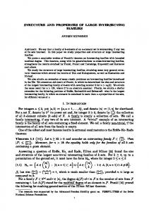
Subsurface fluorescence maxima were widespread in the Canadian High Arctic, Hudson Bay and Labrador fjords during late summer 2005 and early fall 2006 (Fig. 1). Out of 140 stations, 85% clearly showed a subsurface maximum, which ranged broadly in vertical position (7 to 67 m; median: 29 m) and thickness (2 to 74 m; median: 18 m). The other stations (15%) showed vertically homogenous fluorescence (shallow Foxe Basin; 7 to147 m) or a surface maximum (western Baffin Bay, Mackenzie Shelf, inner Canadian Archipelago, Hudson Bay and Labrador fjords). Using the average output of the fluorometer during bottle closure, the relationships between in vivo fluorescence and extracted chl a concentration were assessed separately for each region and expedition (e.g. for Baffin Bay in 2006: y = 1.05x – 0.08; n = 39, r2 = 0.92, p < 0.0001). The small residuals of the regressions showed an even dispersal for concentrations ranging at least 2 orders of magnitude, and intercepts were statistically undistinguishable from zero, indicating negligible interferences or quenching near the surface. Region-specific relationships were used to construct high-resolution vertical profiles of chl a. To determine if cp (λ ≈ 660 nm) is an acceptable surrogate for phytoplankton biomass in Baffin Bay, the biovolume-based estimates of total autotrophic carbon biomass reported by Booth et al. (2002) (determined by epifluorescence microscopy enumeration and sizing) were compared with concomitant transmissometer data (Fig. 2). Strong linear relationships were observed between cp and the carbon biomass of total phytoplankton and diatoms. This exercise was not attempted in the shallow Canadian Archipelago and the coastal Beaufort Sea due to the proximity of the Mackenzie River and resuspension on shallow shelves. The depths of the SCM, the SBM and the oxygen saturation maximum (SOM) were compared in northern Baffin Bay (Fig. 3), where river runoff has a negligible influence on particle load. In 2006 (when the oxygen probe worked consistently and the spatial coverage of northern Baffin Bay was extensive), the vertical depth of the SCM closely matched those of the SBM (when detectable; i.e. when the particle load in surface waters was negligible) and of the SOM. A positive relationship between the depths of the SCM and SOM was also observed in the Beaufort Sea but was much weaker (r2 = 0.24, n = 61) than in Baffin Bay.

0.12

General conditions at the SCM The frequency distributions of physical properties and nitrogenous nutrient concentrations at the SCM depth are presented in Fig. 4. Although irradiance at

Beam attenuation

RESULTS

0.10 0.08 0.06 0.04 0.02 0.00

0

100

200

300

400

Phytoplankton biomass (µg C l–1) Fig. 2. Relationships between particulate beam attenuation (c p) and phytoplankton carbon estimates in northern Baffin Bay (data from late summer 1998; Booth et al. 2002). Model II linear regressions: y = 0.0003x + 0.03, n = 53, r2 = 0.88 (diatom carbon; black circles, dotted line) and y = 0.0002x + 0.03, n = 53, r2 = 0.88 (total autotrophic carbon; gray circles, solid line)

50

50

40

40

30

30

20

20

10

10

0 0

10

20

30

40

SOM (m)

SBM (m)

the SCM ranged from 0.001 to 48% of surface values (daily mean absolute irradiance corresponding to 0.0006–75.12 µmol quanta m–2 s–1 assuming that the mean irradiance along the ship track during a day is representative of a given station), 83% (181 out of 219 CTD stations) of the SCM were located below the 10% light level and the mode of the distribution (52% of the stations) was in the 3 to 10% range (Fig. 4A). Water temperature ranged from –1.5 to 2.0°C at 83% of the

0 50

SCM (m) Fig. 3. Relationships between vertical position of the subsurface chlorophyll maximum (SCM), subsurface biomass maximum (SBM; gray circles) and oxygen saturation maximum (SOM; black circles) for northern Baffin Bay stations in 2006. Model II linear regressions between SBM and SCM depths (solid line: y = 0.96x – 0.93; n = 10, r2 = 0.98) and between SOM and SCM depths (dotted line: y = 1.06x – 3.57; n = 10, r2 = 0.88)

74

Mar Ecol Prog Ser 412: 69–84, 2010

100

50

B

Frequency

A 80

40

60

30

40

20

20

10

0 10

30

10

3

1

3 0.

0. 1

03 0.

01 0.

00 0.

0.

00

1

3

0

–1

0

1

Irradiance (% of incident at surface)

3

4

5

6

7

8

9

35

C

30

25

20

20

15

15

10

10

5

5 0

1

2

3

4

5

6

7

8

9

D

30

25

0

2

Temperature (°C)

35

Frequency

0 –2

10

NO3– (µM)

0 0.0

0.2

0.4

0.6

0.8

1.0

1.2

1.4

NH4+ (µM)

Fig. 4. Frequency distributions of (A) percentage of surface irradiance, (B) water temperature, (C) NO3– and (D) NH4+ concentrations at the depth of the subsurface chlorophyll maximum (SCM). In (C), gray bar = samples below the analytical limit of detection (i.e. < 0.05 µM). All sampling stations and years were pooled

stations (181 out of 219 CTD stations), with a mode between –1.5 and –1.0°C (at 21% of stations; Fig. 4B). Extreme values of –1.8 and 9°C were observed in isolated instances. Nitrate concentrations generally ranged from 0.5 to 3.0 µM with values < 0.5 µM or > 3 µM at 22 and 20% of the stations, respectively (Fig. 4C). NH4+ concentrations varied between the detection limit (0.02 µM) and 1.40 µM with a mode of 0.20 µM at 52% of the stations (Fig. 4D).

Oceanographic sections The positioning of the SCM relative to vertical profiles of nutrients and the physical structure of the water column was explored in detail using 4 oceanographic sections (see Fig. 1 for locations). Concentrations of chl a at the SCM were generally lower in the western sections (Beaufort Sea [BS]: 0.32 to 0.74 µg l–1; Amundsen Gulf [AG]: 0.34 to 2.50 µg l–1) than in the eastern sections (Lancaster Sound [LS]: 0.53 to 4.52 µg l–1;

Baffin Bay [BB]: 1.39 to 16.65 µg l–1) (Fig. 5). There was no consistent regional difference in the depth of the SCM, which most often occurred between 20 and 35 m. Conspicuous exceptions were noted off the shelf break on the BS section (40 to 62 m), at the entrance of LS (70 m) and at 3 stations on the LS and BB sections (12 to 15 m). The SCM was at or well above the 1% surface irradiance in all but 4 stations on the sections. Chl a concentration generally declined to very low values (< 0.1 µg l–1) below the SCM, except in northern BB where they remained moderate (> 0.5 µg l–1) in the upper 80 m of the water column. The pycnocline (i.e. depth with the maximum value of N 2 ) was shallow nearly everywhere (14 to 32 m) but the stratification was stronger in the western sections (i.e. BS and AG) than in the eastern ones (i.e. LS and BB) (Fig. 6A). The pycnocline was systematically located in the upper euphotic zone and most often above the SCM. Oxygen saturation was generally >100% at the SCM, with maximum values generally observed at or close to the SCM (Fig. 6B). NO3–

75

Martin et al.: Subsurface chlorophyll maxima in the Canadian Arctic

Photosynthetic competency Considering the entire sampling area, data from 2005 and 2006 generally displayed high Fv/Fm at the SCM (median: 0.56) although values varied between 0.32 and 0.70 (Fig. 8). At the surface, Fv/Fm ranged from 0.08 to 0.71 with a median value of 0.55 (Fig. 8). The scatter of values was much lower at the SCM than at the surface (where Fv/Fm was frequently < 0.45) and there was no statistically significant difference between the 2 sampling depths (Wilcoxon signed rank test, p = 0.542).

Chl a (µg l–1)

BS

3

20

Depth (m)

concentrations were generally near the analytical detection limit above the SCM, which was typically associated with the top of the nitracline (Fig. 6C). Note that Si(OH)4 and PO43 – concentrations (not shown) followed the same vertical patterns as NO3–, but were not depleted in the surface layer. Maximum NO2– concentrations were much higher in the western sections than in the eastern ones (Fig. 6D). A well-defined primary NO2– maximum (PNM) was visible only in the western sections, where it generally tracked the SCM. In the eastern sections, the layer of elevated NO2– concentration was relatively diffuse and thick with no apparent relationship with the SCM. On all sections, NH4+ concentrations were uniformly low in surface waters and generally showed a subsurface maximum below the SCM (Fig. 6E). Subsurface concentrations were particularly high in the eastern sections (up to 1.24 µM) and elevated NH4+ concentrations extended far below the euphotic zone in northern BB.

40

0.3

60

x x x x xxx x x x x x

80

Light attenuation, nutrients and vertical position of the SCM

0

50

x

100

0.03

150

AG

3

Depth (m)

20 40

0.3

60

x 80 xx 0

x

x

100

x

200

x

x

300

400

x

x

0.03

500

LS

5

Depth (m)

20 40

0.5

60 80

x 0

x 100

x

x

200

x 300

x 400

x 500

x

0.05

600

BB

20

20

Depth (m)

The relationship between the vertical position of the SCM and k for all stations is shown in Fig. 7A. The range of k went from a minimum of 0.046 m–1 at deep stations to a maximum of 0.475 m–1 at neritic stations influenced by large rivers (Fig. 7A). To remove this influence, a model II linear regression was adjusted for stations with k < 0.15 m–1 and showed a very weak (r2 = 0.14), negative relationship between the 2 variables (Fig. 7A). The SCM was deeper than the pycnocline at 86% of the stations and no significant correlation was observed between their respective vertical positions (Fig. 7B). However, 68% of the stations showed a vertical match between the depth of the SCM and the nitracline within a margin of ±10 m (Fig. 7C). This match extended to 90% of the stations for a margin of ± 20 m. A linear regression fit trough all data evidenced 16 large residuals (standardized residuals ≥ 2; belonging to stations with poorly defined SCM or nitracline) that belonged to either very weakly stratified stations (maximum N 2 ≤ 0.0006) or sites where the nitracline was more than 12 m below the 1% of surface irradiance (Fig. 7C). The regression was largely improved by removing the outliers from the analysis. To verify if light penetration through the upper water column improved the relationship, a multivariate linear regression model considering the depth of the SCM, k (x1) and the depth of the nitracline (x2) was adjusted to stations where k < 0.15 m–1 (minus the 16 outliers). A relationship was obtained (y = –36.67x1 + 0.775x2 + 10.92; r2 = 0.67, p1 = 0.2260, p2 < 0.0001), but the regression coefficient for k was not significant.

40

2

60

x

80 0

x

x 50

x x

x 100

x

x

x

0.2

150

Distance (km) Fig. 5. Vertical variations of calibrated chl a concentration (right-hand color key) along sections in BS, AG, LS and BB (see Fig. 1 for exact locations). Dashed and solid lines: depths of the subsurface chlorophyll maximum and of the euphotic zone (defined here as 1% of surface irradiance), respectively. Position of each sampling station: ‘x’ on the bottom axis

x

x

x

x

x

x

x

0

x

x

x

x

300

x

x

x

x

0

x

x

x

x x

100

Baffin Bay

x

x

x

x

3

4

Depth (m) 150 0

100

200

300

400

100

Distance (km)

500

200

400

500 600

50

150

0

0.2

0.4

Fig. 6. Vertical variations of (A) Brunt-Väisälä frequency (N 2), (B) percent oxygen saturation (O2 sat), (C) NO3–, (D) NO2– and (E) NH4+ concentrations along sections in Beaufort Sea, Amundson Gulf, Lancaster Sound and northern Baffin Bay. Note the different depth scale for N 2 and O2 sat (0–80 m). See Fig. 5 for definition of lines and symbols. White areas: no data; Grey areas: bottom of water column

100 NH + 4 (µM) x x x x xxx x x x x x 150 0 50 100

0.8 0.6

50

0.1

0.2

0.3

0

5

1

NO2– (µM)

NO3– (µM)

10

15

80

90

100

110

0

E

150

100

50

D

150

100

50

C

60 O2 sat (%) 80

40

20

B

1

xx x

Lancaster Sound

60 N (x10–3 s–2) 80

x

Amundsen Gulf

2

2

Beaufort Sea

40

20

A

76 Mar Ecol Prog Ser 412: 69–84, 2010

77

Martin et al.: Subsurface chlorophyll maxima in the Canadian Arctic

Taxonomic composition at the SCM

80

A

70

50 40 30 20 10 0 0.0

0.1

0.2

0.3

0.4

0.5

k (m–1) 80

B

70

SCM (m)

60 50 40 30 20 10 0 0

10

20

30

40

50

60

70

80

Pycnocline (m) 80

C

70

SCM (m)

60 50

The taxonomic composition of the phytoplankton at the SCM was investigated for both sampling years (Fig. 9). The relative abundance of flagellates and dinoflagellates was 21 and 38% lower, respectively, in 2006 than in 2005 in all regions. During both years, the BS presented lower percentage of diatoms and higher percentages of flagellates and dinoflagellates than northern BB. Flagellates and dinoflagellates were numerically dominant in the Hudson Bay system in 2005 and made up, on average, 90% of the total phytoplankton abundance. In all regions, centric diatoms were, on average, 3 to 27 times more abundant than pennate diatoms. Except in the Hudson Bay system, Chaetoceros spp. were the most abundant centric diatoms at the SCM in 2005 and 2006 (76 to 99% of total centric diatoms on average). Chaetoceros socialis Lauder was present at 56% of the stations and represented up to 30% of the total Chaetoceros abundance. However, C. socialis was less abundant in 2006 than in 2005. Diatoms of the genus Thalassiosira were scarce throughout the Canadian Arctic (0 to 0.5%). Pearson’s product moment correlations (PPMC) were used to evaluate relationships between environmental variables and the relative and absolute abundance data. Only the significant correlations are described here. At the SCM, the absolute abundance of flagellates increased with NH4+ concentration (r = 0.48, p < 0.01). The relative abundance of dinoflagellates increased with N 2 (r = 0.32, p < 0.05), whereas the relative abundance of pennate diatoms increased with NO2– concentration (r = 0.39, p < 0.01). The relative dominance of diatoms over flagellates decreased with water temperature (r = –0.34, p < 0.05) and increased with ambient NO3– concentration (r = 0.31, p < 0.05).

40 30

35

20

30

10 0

0

10

20

30

40

50

60

70

80

Nitracline (m) Fig. 7. Relationships between depth of the subsurface chlorophyll maximum (SCM) and (A) the coefficient of diffuse light attenuation (k), (B) the pycnocline, and (C) the nitracline in 2005 (black circles) and 2006 (gray circles). In (A), vertical dash-dotted line: k = 0.15 m–1 (see ‘Results: Light attenuation, nutrients and vertical position of the SCM’ for details); and dashed line: model II linear regression for stations, where k < 0.15 m–1 (y = –594.5x + 96.18; r2 = 0.14). In (B) and (C), solid line indicates 1:1 match; and dashed line: model II linear regression between SCM and pycnocline depths (y = 1.18x + 13.86; r2 = 0.04) and between SCM and nitracline depths (y = 0.98x – 0.16; r2 = 0.66 when excluding 16 outliers). Dashdotted lines in (C) represent 1:1 ± 20 m

Frequency (%)

SCM (m)

60

25 20 15 10 5 0

0.1

0.2

0.3

0.4

0.5

0.6

0.7

Fv /Fm Fig. 8. Frequency distribution of Fv/Fm at the surface (black) and at subsurface chlorophyll maximum (gray). All sampling stations and years were pooled

78

Mar Ecol Prog Ser 412: 69–84, 2010

Beaufort Sea

Canadian Archipelago

Hudson Bay

Baffin Bay

1.7

2005

0.1 5.9 0 4.8

4.8 1.1

0.2 0.2

0.5 0.1

2.1

0 3.6

0.1 5.0

2.0

3.9

19.0 19.0

18.8 18.8 7.2 7.2

8.1 8.1 1.0

3.3

68.7 68.7

67.3 67.3

83.3 83.3

87.3 87.3 68.7%

83.3%

2006 8.8 0.4

3.1

4.1

Dinoflagellates

0 0.5

7.7 6.9

Flagellates

13.3

Pennate diatoms

20.3 35.4 0

29.9

45.2

Chaetoceros spp.

37.1 8.9

Chaetoceros socialis

55.9

8.0 7.1 7.1

Thalassiosira spp. Other centric diatoms

2.8 4.8 Fig. 9. Mean percent abundance of the major phytoplankton groups observed at the depth of the subsurface chlorophyll maximum in the Beaufort Sea, inner Canadian Archipelago, northern Baffin Bay and Hudson Bay in 2005 and 2006. Hudson Bay was not sampled in 2006

NO3– concentration was positively correlated to NO2– concentration (r = 0.52, p < 0.001) and salinity (r = 0.30, p < 0.05).

DISCUSSION This study provides the first near-synoptic assessment of the incidence and properties of SCM through the Canadian Arctic, including the subarctic Hudson Bay and Labrador fjords, during late summer and early fall. Results show that SCM are almost ubiquitous and imply that they persist throughout the ice-free period since they are known to appear early in the growth season (Booth et al. 2002, Tremblay et al. 2008). Now that the prevalence of SCM is established, their characteristics will be discussed with respect to the physico-chemical structure of the water column, potential repercussions for the estimation of primary production by remotesensing and biogeochemical implications. The absence of SCM was noted only near rivers and at shallow locations (