network with Poisson arrivals and arbitrary holding time distributions. .... pricing schemes, the network has prior knowledge of the individual service time of.
Pricing-Based Control of Large Networks Xiaojun Lin and Ness B. Shroff School of Electrical and Computer Engineering Purdue University, West Lafayette, IN 47906, USA {linx, shroff}@ecn.purdue.edu
Abstract. In this work we study pricing as a mechanism to control large networks. Our model is based on revenue maximization in a general loss network with Poisson arrivals and arbitrary holding time distributions. In dynamic pricing schemes, the network provider can charge different prices to the user according to the current utilization level of the network. We show that, when the system becomes large, the performance of an appropriately chosen static pricing scheme, whose price is independent of the current network utilization, will approach that of the optimal dynamic pricing scheme. Further, we show that under certain conditions, this static price is independent of the route that the connections take. This result has the important implication that distance-independent pricing that is prevalent in current domestic telephone networks in the U.S. may in fact be appropriate not only from a simplicity, but also a performance point of view. We also show that in large systems prior knowledge of the connection holding time is not important from a network revenue point of view.
1
Introduction
In the last few years there has been significant interest in using pricing as a mechanism to control communication networks. The network uses the current price of a resource as a feedback signal to coerce the users into modifying their actions (e.g. changing the rate or route). Price provides a good control signal because it carries monetary incentives. Past works in the literature differ in their schemes to compute the price. Some of the proposed schemes use different forms of auctions, e.g., “Smart Market” [9] or “Progressive Second Price Auction” [7] to reach the right price. Other schemes use differential equations at the resource and at the users to converge to such prices [4]. A common theme behind this category of research is to have the resource calculate price based on the instantaneous load and available capacity. If the current condition changes, a new price is calculated. The users are expected to act on up-to-date price information to achieve the desired design objectives. Feedback delays to the user may introduce undesirable effects on the performance of the system, such as instability or slow speed of convergence [4]. In practice, this feedback delay may be difficult to control because calculating up-to-date price information continuously consumes a large amount of processing power at
the resource/node. Also, there is a substantial communication overhead when users try to obtain these up-to-date prices. Pricing over multiple resources also poses additional problems. Usually the price is calculated over a given route by summing over the price of all the resources along that route [4, 8, 14]. The user has to act on the sum. This kind of route-specific or distance-specific price may introduce substantial signaling overhead in real networks. Interestingly, in our daily lives, we observe quite the opposite phenomenon. For example, we do not see the prices of products we purchase everyday fluctuate substantially, but in fact they change very slowly. Another example of distanceneutral pricing is the domestic long distance telephone service in the US. Most long distance companies offer flat rate pricing to users calling anywhere within the continental US. These observations have motivated a number of recent works. In [12], after a critique on the optimality-pricing approach, the authors have proposed two approximations of congestion pricing: the first approximation was to replace the instantaneous congestion conditions1 by the expected or average congestion conditions, similar to time-of-day pricing. The second approximation was to replace the cost of the actual path the flow would traverse through the network with the cost of the expected path; where the charge depends only on the source and destination(s) of the flow and not on the particular route taken by the flow. However, in this work, there is no analysis of the performance implication of such approximations. In [11], the authors investigate this problem in the case of a single resource with Poisson arrivals and exponential service times. In particular, the authors study the expected utility and revenue under both dynamic pricing and static pricing schemes in a dynamic network. By a dynamic network, we mean that in their system, call arrivals and departures are taken into account. This is different from the work in [4, 6, 8, 14] where the authors view congestion control as a distributed asynchronous computation to maximize the aggregate source utility. In these works, the optimization is done over a snapshot in time, i.e., it does not take into account the dynamic nature of the network. In contrast, in [11], the authors model the dynamic nature of the system by assuming that calls arrive according to a Poisson process and stay in the system for an exponentially distributed time. The authors study the expected utility and revenue under both dynamic pricing and static pricing schemes. It is shown that when the capacity is large, using a static pricing scheme suffices, in the sense that the utility (or revenue) under an appropriately chosen static price converges asymptotically to that of the optimal dynamic scheme. The implication of this work is that we can now base pricing decisions only on the average load rather than on the instantaneous load, thus reducing both processing and communication overhead. This paper extends the results in [11] in two directions: 1
Note that the congestion conditions in [12] can be obtained from the instantaneous load and available capacity in the system. Hence, these terms can be viewed interchangeably.
1) We show that the same type of invariance results hold for general loss networks (i.e., the performance of the optimal static pricing scheme asymptotically approaches the performance of the dynamic scheme). The results hold even if the service time distribution is general. We show that the right static price depends on the service time distribution only by its mean. These extensions have two implications: Firstly, while the assumption of Poisson arrivals for calls or flows in the network is usually considered reasonable, the assumption of exponential holding time distribution is not. For example, much of the traffic generated on the Internet is expected to occur from large file transfers which do not conform to exponential modeling. By weakening the exponential service time assumption we can extend our results to more realistic systems. Secondly, in the general network case, we can show that in our revenue-maximization problem, under certain conditions, the static price only depends on the price elasticity of the user, and not on the specific route or distance. This indicates that the flat pricing scheme used in the domestic long distance service in the US may, in many cases, be good enough. 2) Thus far, when we refer to dynamic pricing schemes, we mean schemes that take into account the current congestion information. We now consider an even broader set of dynamic pricing schemes and show that the performance of the static pricing scheme suffices for large systems. In this broader set of dynamic pricing schemes, the network has prior knowledge of the individual service time of the connections when they arrive. The question is whether we can gain additional advantage by pricing the resource based on this additional information. Our analysis shows that when the system grows large, this additional information does not result in significant gain. We show that the individual service time is inessential, and a static price based on the average service time suffices. We believe that these results are important in understanding how to use pricing as a mechanism for controlling real networks. The possibility of using static and/or route-independent prices will give rise to more efficient and realistic algorithms. Also, “pricing” here can be interpreted as a general signal which is only loosely related to actual pricing. For example, pricing models have been used as a mechanism to understand resource allocation and congestion control. Therefore the results we present here will help us in better understanding how to control large networks. 1.1
Related Work
The ideas of upper bounding the performance of the optimal dynamic policy in a general loss network and showing that fixed/static policy approaches the upper bound asymptotically have been reported in the past, for example, [10, 5], and the reference therein. In their work, the objective to be optimized is a linear function of the number of users in the system, i.e., the utility value. This objective function maximizes the utilization of the network, but does not consider the revenue generated, hence there is no notion of the price of a resource. Maximizing the utility in a system corresponds to a linear optimization problem. However, revenue maximization is more difficult to evaluate because it is a non-linear
optimization problem. Moreover, users can easily take advantage of the system by providing an incorrect utility value when price is not an issue. Pricing is a mechanism to coerce users into using the amount of resources that they need (or can afford!). Recently, in [11], Paschalidis and Tsitsiklis have investigated the problem of revenue maximization. Our work extends the result of [11] to general loss networks and general service time distributions. Further, our proof of the stationarity and ergodicity of such types of system with feedback control is new, and of value in its own right. Our treatment of pricing schemes based on the call duration sheds insight on the optimal dynamic policy. The rest of the paper consists of three parts. In Sect. 2, we investigate the case of a general loss network with Poisson call arrivals and general service time distribution. In Sect. 3, we study the implication of individual service time on the price and in Sect. 4, we conclude.
2 2.1
General Loss Network, General Service Time Model
Consider an abstract network providing service to multiple classes of users. There are L links in the network. Each link l = {1, ..., L} has capacity Rl . There are I classes of users. For users of each class i, there is a route through the network. The routes are characterized by a matrix {Cil , i = 1, ..., I, l = 1, ..., L}, where Cil = 1 if the route of class i traverses link l, Cil = 0 otherwise. Each class i connection consumes bandwidth ri . A call is rejected and lost if any of the links it traverses does not have enough capacity to accommodate it, otherwise it may be admitted to the network depending on the network policy. Calls of class i arrive to the network according to a Poisson process with rate λi (ui ), which is a function of the price ui charged to users of class i. Here ui is defined as the price per unit time of connection. We assume that λi (ui ) is a non-increasing function of ui . Therefore λi (ui ) represents the price-elasticity of class i. Once admitted, the call will hold the resources on all links it traverses until it finishes service. The service time distribution is general with mean 1/µi . The network provider can charge different prices for different classes of users. A dynamic price is one where charges are based on the current utilization of the resource, for example, how many calls of each class are already in service, and how long they have been served, etc. On the other hand, a static price is one which only depends on the class of the user and is indifferent to the current utilization of the resource. 2.2
Stability of the Model
Our first result is regarding the stability of such a system. Note that our model is very similar to a network of M/G/N/N queues. However, here we also have “feedback” introduced by the price ui , which makes the model somewhat more complex. The arrival rate is changing over time. It is not intuitive to even define
stationarity and ergodicity for the input! However, as we will see next the system will be stationary and ergodic under very general conditions. Proposition 1. Assume that the arrival rates λi (u) are bounded above by some constant λ0 for all classes i, the service times are i.i.d. with finite mean and independent of the arrivals. If the price is only dependent on the current state of the system, then any stochastic process that is only a function of the system state is asymptotically stationary and the stationary version is ergodic. Proof. To show this, let us first look at the case of a single resource with users coming from a single class i. To develop the result, we need to take a different but equivalent view of the original model. In the original system, the arrival rate is a function of the current price. In the new but equivalent system, the arrival rate is constant but is thinned by a probability as a function of the price. Specifically, in the new model, the arrivals are Poisson with constant rate λ0 . Each arrival now carries a value v that is independently distributed, with distribution function P {v ≥ u} = λi (u)/λ0 . The value v of each arrival is independent of the arrival process and service times. If v < u, where u is the current price at the time of arrival, the call will not enter the system. We can see that with this construction, at each time instant, the arrivals are bifurcated with probability of success equal to P {v ≥ u} = λi (u)/λ0 . Therefore the resultant arrivals (after thinning) in the new model are also Poisson with rate λ0 P {v ≥ u} = λi (u). Thus the model is equivalent to the original model. To show stationarity and ergodicity, we need to construct a so called “regenerative event” [1]. Let {τne , τns , vn }, −∞ < n < ∞, be the n-th arrival’s interarrival time, service time, and value, respectively (note this is the arrival of the Poisson process before bifurcation.) Let s s e s Qn = 1{ τn−1 < τne } + 1{ τn−2 < τne + τn−1 } + ... + 1{ τn−k
0. Proof. See Appendix. Now by Borovkov’s Ergodic Theorem, [1], the distribution of the state of the system converges as n → ∞ to the distribution of the stationary process. Ergodicity follows from the lemma below.
Lemma 2. The regenerative event An is positive recurrent, i.e., let T1 = inf{Xn ∈ An }. Then E{T1 |X0 ∈ A0 } < ∞, where Xn is the state of the system at time n. Proof. See Appendix. Since the regenerative event is positive recurrent, the state of the system is both stationary and ergodic, i.e., any random process that depends only on the state of the system is both stationary and ergodic [13]. For the case of multiple classes and multiple links, assume there are I classes. We can construct the equivalent system in the following way: we first construct Poisson arrivals with rate Iλ0 . Each of these arrivals is assigned to class i with probability 1/I, and each of these assignments is independent of each other. The service time is then generated according to the service time distribution of class i. Each class i arrival carries a value v that is independently distributed, with distribution function Pi {v ≥ ui } = λi (ui )/λ0 . The value v of each arrival is independent of the arrival process and service times. If v < ui where ui is the current price for class i at the time of the arrival, the call will not enter the system. Following the same idea as in the first paragraph of the proof, it is easy to show that such a constructed system is equivalent to the original system. The initial Poisson arrivals with rate Iλ0 can be interpreted as “all potential arrivals from all classes.” Let {τne , τns } be the n-th arrival’s interarrival time and service time respectively. It then follows that the sequence of service times τns is again i.i.d. with finite mean, and it is independent of the arrivals. Hence, we can construct the event A0 as before, which is now the event that “all potential arrivals from all classes have left the system before time n.” Again this event is the “regenerative event” for the system, and we can show that P {A0 } > 0, and A0 is positive recurrent. Therefore, the system is asymptotically stationary and the stationary version is ergodic. t u 2.3
Dynamic Price, Static Price, and Upper Bound
In this section, we consider dynamic pricing schemes that are based on the current occupancy of the network resources. Let n = {ni , i = 1, ..., I} represent the state of the network, where ni is the number of users from class i that are being P served in the network. Let Ω denote the set of possible states, then Ω = {n : i ni ri Cil ≤ Rl for all l}. Let n(t) denote the state at time t, then the dynamic price for class i can be written as ui (t) = gi (n(t)), where gi is a function from Ω to the set of real numbers R. Let g = {gi , i = 1, ..., I}. The expected revenue achieved by any dynamic pricing scheme is given by "Z # I T X 1 1 lim E λi (ui (t))ui (t) dt . T →∞ T µi 0 i=1 From stationarity and ergodicity established in the last section, we have "Z # � � I I T X X 1 1 1 lim E λi (ui (t))ui (t) dt = E λi (ui (t))ui (t) , T →∞ T µi µi 0 i=1 i=1
where the right hand side is independent of t (because of stationarity). Therefore, the optimal dynamic policy is � � I X 1 J ∗ = max . E λi (ui (t))ui (t) g µi i=1
On the other hand, for static pricing schemes, the expected revenue per unit time is: I X 1 J0 = λi (ui )ui (1 − Ploss,i [u]), µ i i=1 where Ploss,i [u] is the probability of loss for class i when the price vector is u = [u1 , ..., uI ]. Therefore the optimal static policy is Js = max u
I X
λi (ui )ui
i=1
1 (1 − Ploss,i [u]). µi
∗
By definition Js ≤ J . Here we show that the upper bound in [11] is also an upper bound for our case. For convenience, we write ui as a function of λi . Let Fi (λi ) = λi ui (λi ) µ1i . Let Jub be the optimal value of the following nonlinear programming problem: X max Fi (λi ) (1) λi
subject to
i
λi = µi ni for all i X ni ri Cil ≤ Rl for all l.
(2)
i
Proposition 2. If the functions Fi are concave, then J ∗ ≤ Jub . Proof. We follow the same method as in the proof of Theorem 6 in [11]. Consider an optimal dynamic pricing policy. Let ni (t) be the number of calls of class i in the system at time t. View λi (t) and ni (t) as random variables. From Little’s Law, we have 1 E[ni (t)] = E[λi (t)] . µi P At any time t, i ni (t)ri Cil ≤ Rl for all l. Therefore " # X X l l E[ni (t)ri Ci ] ≤ E ni (t)ri Ci ≤ Rl for all l. (3) i
i
Therefore λi = E[λi (t)] and ni = E[ni (t)] satisfy the constraint of Jub . Using the concavity of F and Jensen’s inequality, we have X X Jub ≥ Fi (E[λi (t)]) ≥ E [Fi (λi (t))] = J ∗ . i
i
t u
2.4
The Many Sources Regime
Consider the regime of many small users. Let c ≥ 1 be a scaling factor. We consider a series of systems scaled by c. The scaled system has capacity Rc = cR, c and the arrivals of each class i has rate λci (u) = cλi (u). Let J ∗,c , Jsc and Jub be the dynamic revenue, static revenue, and upper bound, respectively, for the c-scaled system. Proposition 3. If the functions Fi are concave, then 1 c 1 1 c . Js = lim J ∗,c = lim Jub c→∞ c c→∞ c c→∞ c P c Proof. Firstly, P Jub isl obtained lby maximizing i cλi ui (λi )/µi , subject to the constraint i cλi ri Ci /µi ≤ cR for all l. Therefore the optimal price is indec = cJub . pendent of c, and Jub c Now consider Js , for every static price uci falling into the constraint of Jub , i.e., X cλi (uc )ri C l i i ≤ cRl for all l, (4) µ i i lim
let J0c denote the revenue under this static price. We will show that as c → ∞, J0c X 1 λi (uci )uci . = c→∞ c µi i lim
(5)
If we take the optimal price of the upper bound as our static price, then the right hand side of (5) is exactly the upper bound. Therefore, Jsc Jc ≥ lim 0 ≥ Jub . c→∞ c c→∞ c lim
On the other hand, Jsc ≤ J ∗,c ≤ cJub , and the result follows. Now we show (5). The key idea is to use an insensitivity result from [3]. In [3], Burman et. al. investigate a blocking network model, where a call instantaneously seizes channels along a route between the originating and terminating node, holds the channels for a randomly distributed length of time, and frees them instantaneously at the end of the call. If no channels are available, the call is blocked. When the arrivals are Poisson and the holding time distributions are general, the authors in [3] show that the blocking probabilities are still in product form, and are insensitive to the call holding-time distributions. This means that they depend on the call duration only through its mean. Our system is a special case of [3]. Let n = {nj , j = 1, ..., I} be the vector denoting the state of the system, and let λj be the arrival rate of class j under the static price ucj , i.e., λj = cλj (ucj ). Let ρj = λj /µj . From [3], we have the blocking probability of calls of class i as: P Q nj ρj /nj ! n∈Γ 0 j c Ploss,i = P Q nj , (6) ρj /nj ! n∈Γ0 j
where Γ0 =
X
nj rj Cjl ≤ cRl for all l and there exists an l
j
such that Cil = 1 and
Γ0 =
X
X
nj rj Cjl > cRl − ri
j
nj rj Cjl ≤ cRl for all l
j
.
Since from (6) we can see that the blocking probability is exactly the same as in the case of exponential service times, we now only need to look at the case of exponential service times. Consider an infinite channel system with the same arrival rate and holdingtime distribution. Let nj,∞ be the number of flows of class j in the infinite channel system. Further let n∞ = {nj,∞ , j = 1, ..., I} be the vector denoting the c state of the infinite channel system. We can then rewrite Ploss,i as c Ploss,i = PΓc,∞ /PΓc,∞ , 0 0
where
P Q PΓc,∞ = 0
n∞ ∈Γ0 j
e
P Q
n
ρj j,∞ /nj,∞ !
P j
ρj
and PΓc,∞ = 0
n∞
∈Γ 0
j
n
ρj j,∞ /nj,∞ !
P
e
j
ρj
are the probabilities that {n∞ ∈ Γ0 } and {n∞ ∈ Γ 0 }, respectively in the infinite channel system. c We will use the estimate of PΓc,∞ and PΓc,∞ to bound Ploss,i . In the infinite 0 0 channel system, there is no constraint. Therefore the number of flows nj,∞ in class j is Poisson (from well known M/M/∞ result) and independent of the number of flows in other classes. We can view each nj,∞ as a sum of c independent random variables. First we calculate the first and second order statistics of nj,∞ . E[nj,∞ ] = c
λj , µj
σ2 [nj,∞ ] = c
λj . µj
Now by invoking the Central Limit Theorem, as c → ∞, we have λ
nj,∞ − c µjj λj √ → N (0, ) µj c
in distribution.
(7)
P l Let xc,l ∞ , j nj.∞ rj Cj be defined as the amount of resource consumed at link l in the infinite channel system. We have X λj X λj E[xc,l rj Cjl , σ2 [xc,l rj2 Cjl . ∞] = c ∞] = c µ µ j j j j
Therefore
c,l P λj l x∞ − r C j µ j j c q j → N (0, Q) in distribution, 1 c
where Q = {Qmn },
Qmn =
X λj j
Now since
P
λ
j
c µjj rj Cjl ≤ cRl
µj
(8)
rj2 Cjm Cjn .
for all l (4),
�
� xc,l ∞ ≤ Rl , for all l c→∞ c xc,l X λ j ∞ rj Cjl , for all l (by (4)) ≥ lim inf P ≤ c→∞ c µj j � � λj ≥ lim inf P nj,∞ ≤ c , for all j (by definition of xc,l ∞) c→∞ µj � Y � λj = lim inf P nj,∞ ≤ c ≥ 0.5I (by (7)) , c→∞ µ j j
lim inf PΓc,∞ = lim inf P 0 c→∞
� lim sup PΓc,∞ 0 c→∞
= lim sup P c→∞
xc,l ∞ ≤ Rl , for all l, and there exists l c Cil
xc,l ri = 1 and ∞ > Rl − c c
�
such that � X � xc,m xc,l ri ∞ ∞ ≤ lim sup P ≤ Rm , for all m, and > Rl − c c c c→∞ l � � X ri xc,l ≤ lim sup P Rl − < ∞ ≤ Rl c c c→∞ l r i X 1 √ q Pc ≤ lim sup (by (8)) (9) λj 2 l c→∞ 2π 1 r C l j j j µj c X = 0 = 0. l
Therefore c lim Ploss,i = lim PΓc,∞ /PΓc,∞ = 0, 0 0
c→∞
c→∞
and X X Jsc Jc 1 1 c ≥ lim 0 = lim λi (uci )uci (1 − Ploss,i )= λi (uci )uci . c→∞ c c→∞ c c→∞ µi µi i i lim
Thus the result follows.
t u
The above proof not only shows that the limit converges, but also shows that the speed of convergence is at least √1c . To see this, we go back to (9). The convergence is the slowest when (4) is satisfied with equality, in which case ri X 1 X 1 1 √ q Pc √ √ qP ≤ λj 2 l 2π 1 2π c r C l l j µj j
c
j
ri λj l j µj rj Cj
mini ri
In fact, we can show that if the maximizing price of the upper bound falls inside the constraint (4), (instead of at the border), then the speed of convergence is exponential. Here we report a few numerical results. Consider the network in Fig. 1. There are 4 classes of flows. Their routes are shown in the figure. Their arrivals are Poisson. The function λi (u) for each class i is of the form � � λi (u) = λmax,i 1 −
u
��+
umax,i
,
i.e., λi (0) = λmax,i and λi (umax,i ) = 0 for some constants λmax,i and umax,i . The price elasticity is then −
1/umax,i λ0i (u) = , for 0 < u < umax,i . λi (u) 1 − u/umax,i
The mean holding time is 1/µi. The arrival rates, price elasticity, service rates µi , and bandwidth requirement are shown in Table 1.
L1
Class 1
L4 L3
Class 2 L2
Class 3
Class 4 L5
Fig. 1. The network topology
First, let us consider a base system where the 5 links have capacity 10, 10, 5, 15, and 15 respectively. The solution of the upper bound (1) is shown in Table 2. The upper bound is Jub = 127.5. We then use simulations to verify how tight this upper bound is and how close the performance of the static pricing policy can approach this upper bound when the system is large. We use the price induced
Table 1. Traffic and price parameters of 4 classes
Class 1 Class 2 Class 3 Class 4 λmax,i 0.01 0.01 0.02 0.01 umax,i 10 10 20 20 Service Rate 0.002 0.001 0.002 0.001 Bandwidth 2 1 1 2
Table 2. Upper bound in the constrained case, Jub = 127.5 Class 1 Class 2 Class 3 Class 4 ui 9.00 5.00 12.00 10.00 λi 0.00100 0.00500 0.00800 0.00500 5.00 4.00 5.00 λi /µi 0.500
by the upper bound calculated above as our static price. We first simulate the case when the holding time distributions are exponential. We simulate c-scaled versions of the base network where c ranges from 1 to 1000. For each scaled system, we simulate the static pricing scheme, and report the revenue generated. In Fig. 2 we show the normalized revenue J0 /c as a function of c. As we can see, as the system grows large, the performance gap between the static pricing scheme and the upper bound gets smaller and smaller. Although we do not know what the optimal dynamic policy is, its normalized revenue J ∗ /c must lie somewhere between that of the static policy and the upper bound. Therefore the performance gap between the static pricing scheme and the optimal dynamic scheme also gets very small. For example, when c = 10, which corresponds to the case when the link capacity can accommodate around 100 flows, the performance gap between the static √ policy and the upper bound is less than 7%. Further the gap decreases as 1/ c. Now, we change the capacity of link 3 from 5 to 15. The solution of the upper bound is shown in Table 3.
Table 3. Upper bound in the unconstrained case, Jub = 137.5
Class 1 Class 2 Class 3 Class 4 ui 5.00 5.00 10.00 10.00 λi 0.00500 0.00500 0.0100 0.00500 5.00 5.00 5.00 λi /µi 2.50
Jo/c 130 125 120 115 110 105 100 95
1
10
100
1000
c: scaling Fig. 2. The static pricing policy compared with the upper bound: the constrained case. The dotted line is the upper bound.
The upper bound is J ∗ = 137.5. The simulation result (Fig. 3) confirms again that the performance of the static policy approaches the upper bound when the system is large. At c = 10, the performance gap between the static policy and the upper bound is less than 10%. Also note that when the system is in an unconstrained state, the price in our static scheme is the same for users with the same price-elasticity even if they traverse different routes. For example, classes 1 & 2 and classes 3 & 4 have the same price (and price-elasticity) but have different routes. In general, if there is no significant constraint of resources, the maximizing price structure will be independent of the route of the connection. To see this, we go back P to the formulation of the upper bound (1). If the unconstrained maximizer of i Fi (λi ) satisfies the constraint, then it is also the maximizer of the constrained problem. In this case the price only depends on the function ui (λi ), which represents the price elasticity of the users. Readers can verify that in our second example when the capacity of link 3 is 15, if we lift the constraints in (2), and solve the upper bound again, we will get the same result. Therefore in our example, the optimal price will only depend on the price elasticity of each class and not on the specific route. Since class 1 has the same price elasticity as class 2, its price is also the same as that of class 2, even though it traverses a longer route through the network. That also explains why in some scenarios, for example, state-to-state long distance in US, prices are flat. We also simulate the case when the holding time distribution is deterministic. The result is the same as that of exponential holding time distribution. The case with heavy tail holding time distribution is more complicated. Here is a result when the holding time distribution is Pareto, i.e., the cumulative distribution function is 1 − 1/xa , with a = 1.5. This distribution has finite mean but infinite variance. We use the same set of parameters as the constrained case above,
Jo/c 140
130
120
110
100
1
10
100
1000
c:scaling Fig. 3. The static pricing policy compared with the upper bound: the unconstrained case. The dotted line is the upper bound.
and let the Pareto distribution have the same mean as that of the exponential distribution. In Fig. 4, we can see that even with the Pareto distribution the performance of the static policy still follows the same trend as the case of exponential holding time distribution. It demonstrates that our result is indeed invariant of the holding time distribution. However, we also note that if the holding time distribution is Pareto with infinite variance, the sample path convergence becomes very slow. The problem is even worse when the system is large. We will briefly discuss this in the conclusion.
3
Pricing on the Incoming Traffic Parameters
Our previous result shows that dynamic pricing based on the instantaneous utilization does not provide us with significant improvement over static pricing, when the system is large. The question to then ask is: If we base our dynamic price on some other factor, can we outperform the static pricing scheme? In this section, we investigate pricing based on another factor, namely the duration of a connection. Thus, here we look at the case when the dynamic pricing scheme, in addition to the instantaneous load, also has prior knowledge of the call duration. For convenience we restrict ourselves to the single resource and single class model. The case of multiple resources and multiple classes can be treated analogously. Assume flows consume unit bandwidth. The only difference from the system studied in Sect. 2 is that now the provider tries to price the incoming call according to additional information, i.e., the duration of the call, (here we assume that each connection request knows how long it has to last). Therefore the
Jo/c 140 130 120 110 100 90
1
10
100
1000
c:scaling Fig. 4. The static pricing policy compared with the upper bound: the constrained case with Pareto distribution. The dotted line is the upper bound. ‘x’ and ‘+’ are 0.99 confidence interval.
price becomes u(t, T ) = g(n(t), T ), where T reflects the length of the incoming call and g is a function from Ω × R to R. The question again is: what is the relationship between such a dynamic pricing scheme and a static pricing scheme? The static pricing scheme can now either take T into consideration (i.e., price is u(T )), or not (i.e., price is u, a constant). In this section we will show that the performance of the static pricing scheme using price independent of T will approach that of the optimal dynamic pricing scheme when the system is large. Therefore there is really no incentive to price according to individual holding time in a large system. We consider the special case when the range of service time can be partitioned into slots [Tk , Tk +∆Tk ), k = 1, 2, ..., and at each time instant the price is constant within each slot, i.e., u(t, T ) = uk (t), u(T ) = uk , for T ∈ [Tk , Tk + ∆Tk ). Let T˜k = E {T |T ∈ [Tk , Tk + ∆Tk )}, and let pk = P {T ∈ [Tk , Tk + ∆Tk )}. Our idea is to decompose the original arrivals into a spectrum of substreams. Substream k has service time [Tk , Tk + ∆Tk ). Its arrival rate is thus λ(u)pk . Here, we assume that the price-elasticity of calls is independent of T . Therefore the arrival of each substream k is still Poisson. The expected dynamic revenue is then given by "∞ # X ∗ ˜ J = max E λ(uk (t))uk (t)Tk pk . g
k=1
The expected static revenue is Js = max uk
∞ X k=1
λ(uk )uk T˜k pk (1 − Ploss ).
where Ploss is the probability that a call is blocked given the static prices uk . Note that this probability is independent of k. Let λk = λ(uk ). Again we write uk as a function of λk . Also let F (λk ) = λk u(λk ). We have, Proposition 4. If F is concave, then J ∗ is upper bounded by Jub , which is the solution of the following optimization problem: Jub = max λk
subject to
∞ X k=1 ∞ X
F (λk )T˜k pk
(10)
λk T˜k pk ≤ R.
(11)
k=1
Also when the system is scaled by c, i.e., λc (u) = cλ(u) and Rc = cR, we have c limc→∞ Jsc /c = limc→∞ J ∗,c /c = limc→∞ Jub /c. Hence, the static price of the form u(T ) = uk , T ∈ [Tk , Tk + ∆Tk ) suffices. Proof. If we view each substream as a class, the only difference from the system we studied in last section is that it has countably infinite number of classes. Since we can still use Little’s Law for each substream, the first part of this proposition can be shown by using the same idea as in the proof of Proposition 2 and by invoking the Monotone Convergence Theorem in (3). In order to show the second part, it suffices to show that when we use the price induced by the upper bound as our static price, Ploss → 0, as c → ∞. Note that as far as Ploss is concerned, the system can be viewed as having only a single class. Therefore, we can reuse the result in the last section. Compared with a system with no pricing control, the arrivals in this system are “weighted” by the static price uk according to their times. Hence, the arrival process is still Pholding ∞ Poisson, with arrival rate�λ0 = k=1 λ(uk )p�k , and the holding time distribution P∞ ˜ Tk λ(uk )pk /λ0 . Because the constraint (11) is is i.i.d. with mean T 0 = k=0
satisfied by such an induced static price, we have λ0 T 0 ≤ R. Using the same techniques as in the proof of Proposition 3, we can show that Ploss → 0 as c → ∞. Then, the result follows. t u Next we study the form of the optimal price uk which maximizes the upper bound (10). We construct another bound J 0 as the solution of the following optimization problem: J 0 = max F (λ) λ
subject to λ
∞ X
T˜k pk
(12)
k=1 ∞ X
T˜k pk ≤ R.
k=1 0
If J = Jub , we will be able to conclude that the optimal λk in (10) should be independent of k, i.e., it is independent of the duration T ! Therefore the price u(T ) should also be independent of T . We now show that this is indeed the case.
From the definition of Jub , J 0 ≤ Jub . It remains to show that J 0 ≥ Jub . For any set of λk that satisfies the constraint of (10), let P∞ ˜ k=1 λk Tk pk λ= P . ∞ ˜ k=1 Tk pk Then λ will satisfy the constraint of (12). Since F is concave, we have P∞ F (λk )T˜k pk F (λ) ≥ k=1 . P∞ ˜ k=1 Tk pk Therefore J 0 ≥ Jub . Now λk is independent of k, and hence, so is uk . We conclude that, in the asymptotic regime, not only is there no incentive to price according to instantaneous utilization, but there is also no incentive to price based on the duration of the individual calls! Again, we recall the previous result, √ that the speed of convergence for this invariance result to hold is at least 1/ c. Our above result suggests that in a very broad sense, the optimal price needs only to take care of one parameter, that is, the traffic class (in a sense the total cost also depends on duration, however the relationship is linear). Note the above result is obtained under the assumption that the arrival elasticity is independent of T . If this is not true, even though the performance of our static price in the form of u(T ) will still approach the performance of the optimal dynamic scheme, u(T ) will not be a constant. In this case, we may need to treat calls of different duration as different classes.
4
Conclusion and Future Work
In this work we study pricing as a mechanism to control large networks. Our model is based on revenue maximization in a general loss network with Poisson arrivals and arbitrary holding time distributions. In dynamic pricing schemes, the network provider can charge different prices to the user according to the varying level of utilization in the network. We prove that this type of a system with feedback is asymptotically stationary and ergodic. We then analyze the performance of the static pricing scheme compared with that of the optimal dynamic pricing scheme. We prove that there is an upper bound on the performance of dynamic pricing schemes, and that the performance of an appropriately chosen static pricing scheme will approach that of the optimal dynamic pricing scheme, when the system is large. Under certain condition, this static price will only depend on the price-elasticity of each class, while being independent of the route of the call. We then extend the result to the case when a network provider can charge a different price according to an additional factor, i.e., the individual holding time. We develop appropriate static pricing schemes for this case and show that the static scheme that is independent of the individual holding time performs as well as the optimal dynamic schemes, when the system is large.
The above results have important implication in the networks of today and in the future. Compared with dynamic pricing schemes, static pricing schemes have some desirable properties. They are less computationally intensive, and consume less network bandwidth. Their performance will not degrade as the network delay grows. Our results show that when the system is large, as in broadband networks, the difference between static pricing schemes and dynamic pricing schemes is minimal. We are currently investigating how to use these results to develop efficient and realistic algorithms to control large networks. We also note that when the holding time distribution is heavy tailed, the sample path convergence to the mean becomes slow. We think this is caused by the fact that with the Pareto distribution, some flows will have very large duration. This fact has two implications on the sample path convergence. One is that the average of the Pareto distributed random variables converges very slowly to their mean, because of a small number of very large samples. The other is that the queue dynamics tend to have correlation over a very large timescale, which leads to very slow convergence of statistics based on queue average. This indicates that the long term average may not be practically meaningful in such cases. The transient behavior might be more important, and deserves to be handled more carefully.
5
Appendix
Proof (of Lemma 1). We follow [1]. To show P {A0 } > 0 , we note that for some a > 0, m ≥ 1, k=m ∞ −1 \ � \ X s s P {A0 } ≥ P {τ0e ≥ a} τ−k ≤a τ−k ≤ τje k=1 k=m+1 j=−k+1 m ∞ −1 \ Y X s s τ−k . = P {τ0e ≥ a} P {τ−k ≤ a}P ≤ τje k=1
k=m+1
j=−k+1
This can be interpreted as the following: A0 is the event that {Q0 = 0}, i.e., all potential arrivals before time 0 has left the system. The event on the right of the inequality above says that, of all the potential arrivals before time 0, the last arrival arrives before a time interval of a, (τ0e ≥ a); the last m arrivals all have service time less than a; and finally, the rest of the arrivals leave the system before time −1. Obviously this is a smaller event than A0 . From now on we will focus on this event only. s Now choose a such that P {τ−k ≤ a} = q > 0, we also have e P {τn ≥ a} = p > 0, since the interarrival times are exponential. Then ∞ −1 \ X s P {A0 } ≥ pq m P τ−k ≤ τje . k=m+1
j=−k+1
Now let B be the event inside the bracket on the right hand side. We only need to show P {B} > 0 for some m. Choose b < E{τne }. Then ∞ −1 [ X s P {B c } = P τ−k > τje k=m+1 j=−k+1 ∞ −1 ∞ [ X [ � s τ−k ≤P τje < b(k − 1) ≥ b(k − 1) k=m+1 j=−k+1 k=m+1 ( ∞ ) ∞ −1 X [ [ e s τj < b(k − 1) +P {τ−k ≥ b(k − 1)} . ≤P k=m+1
j=−k+1
k=m+1
Now as m → ∞, the first term goes to −1 −1 ∞ \ [ X X P τne < b(k − 1) =P τne < b(k − 1) i.o. = 0 m k=m+1
j=−k+1
j=−k+1
by Strong Law of Large Numbers (since b < E{τne }). On the other hand, as m → ∞, the second term goes to ( ∞ ) ∞ [ X s s P {τ−k ≥ b(k − 1)} ≤ P {τ−k ≥ b(k − 1)} → 0 k=m+1
k=m+1
since E{τns } < ∞. Therefore we can choose m large enough such that P {B c } < 1/2. And P {A0 } ≥ pq m P {B} ≥ pq m 1/2 > 0. t u Proof (of Lemma 2). First note that P {Xn ∈ An at least once} = P
(∞ [
) An
.
1
S∞ Again let T be the shift operator, Let B = 1 An , then T B ⊂ B, and P {T B} = P {B}, because B is also a stationary event. Therefore T B and B differ by a set of measure zero, B is an invariant set. Since the arrivals are ergodic, P {B} = 0 or 1. However, since P {B} ≥ P {A0 } > 0, therefore P {B} = 1, i.e., P {Xn ∈ An at least once} = 1. By [2], Prop 6.38. E{T1 |X0 ∈ A0 } =
1 < ∞. P {A0 } t u
References [1] A. A. Borovkov, Stochastic Processes in Queueing Theory, translated by K. Wickwire. New York: Springer-Verlag, 1976. [2] L. Breiman, Probability. Reading, Mass.: Addison-Wesley, 1968. [3] D. Y. Burman, J. P. Lehoczky, and Y. Lim, “Insensitivity of Blocking Probabilities in a Circuit-Switching Network,” Journal of Applied Probability, vol. 21, pp. 850– 859, 1984. [4] F. Kelly, A. Maulloo, and D. Tan, “Rate Control in Communication Networks: Shadow Prices, Proportional Fairness and Stability,” Journal of Operational Research Society, vol. 49, pp. 237–252, 1998. [5] P. B. Key, “Optimal Control and Trunk Reservation in Loss Networks,” Probability in the Engineering and Informational Sciences, vol. 4, pp. 203–242, 1990. [6] S. Kunniyur and R. Srikant, “End-to-End Congestion Control: Utility Functions, Random Losses and ECN Marks,” in Proceedings of IEEE INFOCOM, (Tel Aviv, Israel), 2000. [7] A. A. Lazar and N. Semret, “The Progressive Second Price Auction Mechanism for Network Resource Sharing,” in 8th International Symposium on Dynamic Games and Applications, Maastricht, the Netherlands, pp. 359–365, July 1998. [8] S. H. Low and D. E. Lapsley, “Optimization Flow Control–I: Basic Algorithm and Convergence,” IEEE/ACM Transactions on Networking, vol. 7, no. 6, pp. 861– 874, 1999. [9] J. Mackie-Mason and H. Varian. “Pricing the Internet,”. in Public Access to the Internet, pp. 269–314. The MIT Press, Cambridge, MA, B. Kahin and J. Keller ed., 1995. [10] R. McEliece and K. Sivarajan, “Maximizing Marginal Revenue In Generalized Blocking Service Networks,” in Proc.1992 Allerton Conference on Communication,Control, and Computing, pp. 455–464, 1992. [11] I. C. Paschlidis and J. N. Tsitsiklis, “Congestion-Dependent Pricing of Network Services,” IEEE/ACM Transactions on Networking, vol. 8, pp. 171–184, April 2000. [12] S. Shenker, D. Clark, D. Estrin, and S. Herzog, “Pricing in Computer Networks: Reshaping the Research Agenda,” ACM Computer Communication Review, vol. 26, no. 2, pp. 19–43, 1996. [13] K. Sigman, Stationary Marked Point Processes, An Intuitive Approach. New York: Chapman & Hall, 1995. [14] H. Yaiche, R. Mazumdar, and C. Rosenberg, “A Game Theoretic Framework for Rate Allocation and Charging of Elastic Connections in Broadband Networks,” IEEE/ACM Transactions on Networking, vol. 8, pp. 667–678, Oct. 2000.