Primal-dual nonlinear rescaling method with

Mathematical Programming manuscript No. (will be inserted by the editor) Igor Griva · Roman A. Polyak

Primal-dual nonlinear rescaling method with dynamic scaling parameter update

⋆

Received: / Revised version: Abstract. In this paper we developed a general primal-dual nonlinear rescaling method with dynamic scaling parameter update (PDNRD) for convex optimization. We proved the global convergence, established 1.5-Q-superlinear rate of convergence under the standard second order optimality conditions. The PDNRD was numerically implemented and tested on a number of nonlinear problems from COPS and CUTE sets. We present numerical results, which strongly corroborate the theory.

Key words. Nonlinear rescaling, duality, Lagrangian, primal-dual, multipliers method.

1. Introduction

The success of the primal-dual (PD) methods for linear programming (see [16]-[18], [32]-[34] and references therein) has stimulated substantial interest in the primal-dual approach for nonlinear programming calculations (see [10], [11], [22], [30]). The best known approach for developing primal-dual methods is based on path-following ideology (see e.g. [30]). It requires an unbounded increase of the scaling parameter to guarantee the convergence. Another approach (see [29]) is based on the nonlinear rescaling (NR) methods (see [24]-[28]). The NR method does not require an unbounded increase of the scaling parameter because it has an extra tool to control convergence: the Lagrange multipliers vector. Each step of the NR method alternates the unconstrained minimization of the Lagrangian for the equivalent problem with the Lagrange multipliers update. The scaling parameter can be fixed or updated from step to step. Convergence of the NR method under the fixed scaling parameter allows avoiding the ill-conditioning of ⋆

The research of the authors supported by the NSF Grant CCF-0324999

Igor Griva: Department of Mathematical Sciences, George Mason University, Fairfax VA 22030 Roman A. Polyak: Department of SEOR and Mathematical Sciences Department, George Mason University, Fairfax VA 22030

2

Igor Griva, Roman A. Polyak

the Hessian of the minimized function. Moreover, under the standard second order optimality conditions the NR methods converge with Q-linear rate for any fixed but large enough scaling parameter. To improve the rate of convergence one has to increase the scaling parameter from step to step. Again, it leads to the ill-conditioned Hessian of the minimized function and to a substantial increase of the computational work per Lagrange multipliers update. Therefore, in [29] the authors introduced and analyzed the primal-dual NR method (PDNR). The unconstrained minimization and the Lagrange multipliers update are replaced with solving the primal-dual system using Newton’s method. Under the standard second order optimality conditions, the PDNR method converges with linear rate. Moreover, for any given factor 0 < γ < 1 there exists such a fixed scaling parameter that from some point on just one Newton step shrinks the distance between the current approximation and the primal-dual solution by factor γ. In this paper we show that the rate of convergence can be substantially improved without compromising computational effort per step. The improvement is achieved by increasing in a special way the scaling parameter from step to step. The fundamental difference between the PDNR and the Newton NR methods ([19], [26]) lies in the fact, that in the final phase of the computational process the former does not perform the unconstrained minimization at each step. Therefore the ill-conditioning becomes irrelevant for the PDNR method while for the Newton NR method it leads to numerical difficulties. Moreover, the drastic increase of the scaling parameter in the final stage makes the primal-dual Newton direction close to the corresponding direction obtained by Newton’s method for solving the Lagrange system of equations that corresponds to the active constraints. This is critical for improving the rate of convergence. Our first contribution is the globally convergent primal-dual nonlinear rescaling method with dynamic scaling parameter update (PDNRD). Our second contribution is the proof that the PDNRD method with a special scaling parameter update converges with 1.5-Q-superlinear rate under the standard second order optimality conditions. Our third contribution is the MATLAB based code, which has been tested on a large number of NLP including problems from COPS [5] and CUTE [6] sets. The obtained numerical


⋆⋆

3

results corroborate the theory and show that the PD approach in the NR framework has a good potential to become a competitive tool in the NLP area. The paper is organized as follows. In the next section we consider the convex optimization problem with inequality constraints and discuss the basic assumptions. In section 3 we describe the classical NR multipliers method which has the Q-linear rate of convergence under the fixed scaling parameter. In section 4 we describe and study the PDNRD method. Our main focus is the asymptotic 1.5-Q-superlinear rate of convergence of the PDNRD method. Section 5 describes the globally convergent PDNRD method together with its numerical realization. Section 6 shows the numerical results obtained by testing the PDNRD method. We conclude the paper by discussing issues related to future research.

2. Statement of the problem and basic assumptions

Let f : IRn → IR1 be convex, all ci : IRn → IR1 , i = 1, . . . , m be concave and smooth functions. We consider a convex set Ω = {x ∈ IRn : ci (x) ≥ 0, i = 1, . . . , m} and the following convex optimization problem (P)

x∗ ∈ X ∗ = Argmin{f (x)|x ∈ Ω}.

We assume that: A. The optimal set X ∗ is not empty and bounded. B. The Slater’s condition holds, i.e. there exists xˆ ∈ IRn : ci (ˆ x) > 0, i = 1, . . . , m. Due to the assumption B, the Karush-Kuhn-Tucker’s (K-K-T’s) conditions hold true, i.e. there exists a vector λ∗ = (λ∗1 , ..., λ∗m ) ∈ IRm + such that for the Lagrangian L(x, λ) = f (x) − ∇x L(x∗ , λ∗ ) = ∇f (x∗ ) −

m X i=1

λ∗i ∇ci (x∗ ) = 0,

Pm

i=1

λi ci (x) we have (2.1)

and the complementary slackness conditions λ∗i ci (x∗ ) = 0, i = 1, . . . , m hold true.

(2.2)

4


Let us assume that the active constraint set at x∗ is I ∗ = {i : ci (x∗ ) = 0} = {1, . . . , r}. We consider the vectors functions cT (x) = (c1 (x), . . . , cm (x)), cT(r) (x) = (c1 (x), . . . , cr (x)), and their Jacobians ∇c(x) = J(c(x)) and ∇c(r) (x) = J(c(r) (x)). The sufficient regularity conditions rank∇c(r) (x∗ ) = r, λ∗i > 0, i ∈ I ∗

(2.3)

together with the sufficient condition for the minimum x∗ to be isolated (∇2xx L(x∗ , λ∗ )y, y) ≥ ρ(y, y), ρ > 0, ∀y 6= 0 : ∇c(r) (x∗ )y = 0

(2.4)

comprise the standard second order optimality conditions.

3. Equivalent problem and nonlinear rescaling method

Let −∞ < t0 < 0 < t1 < ∞. We consider a class Ψ of twice continuously differential functions ψ : (t0 , t1 ) → IR, which satisfy the following properties 10 . ψ(0) = 0. 20 . ψ ′ (t) > 0. 30 . ψ ′ (0) = 1. 40 . ψ ′′ (t) < 0. 50 . there is a > 0 that ψ(t) ≤ −at2 , t ≤ 0. 60 . a) ψ ′ (t) ≤ b1 t−1 , b) −ψ ′′ (t) ≤ b2 t−2 , t > 0, b1 > 0, b2 > 0. Let us consider a few transformations ψ ∈ Ψ. 1. Exponential transformation [15] ψ1 (t) = 1 − e−t . 2. Logarithmic MBF [24] ψ2 (t) = ln(t + 1). 3. Hyperbolic MBF [24] ψ3 (t) =

t . 1+t


⋆⋆

5

Each of the above transformations can be modified in the following way. For a given −1 < τ < 0 we define quadratic extrapolation of the transformations 1. − 3. by formulas 4. ψqi (t) =

    ψi (t),

t ≥ τ,

   qi (t) = ai t2 + bi t + ci , t ≤ τ.

where ai , bi , ci we find from the following equations: ψi (τ ) = qi (τ ), ψi′ (τ ) = qi′ (τ ), ψi′′ (τ ) = qi′′ (τ ). We obtain a = 0.5ψ ′′ (τ ), b = ψ ′ (τ ) − τ ψ ′′ (τ ), c = ψ(τ ) − τ ψ ′ (τ ) + τ 2 ψ ′′ (τ ), so ψqi (t) ∈ C 2 . Such modification of logarithmic MBF was introduced in [3] and successfully used for solving large-scale NLP (see [2], [3], [7], [20]). It is easy to check that transformations 1. − 4. satisfy properties 10 − 60 . Modification 4. leads to transformations, which are defined on (−∞, ∞) and along with penalty function properties, have some extra important features. One can find other examples of transformations with similar properties in [1], [3], [25]. For any given transformation ψ ∈ Ψ and any k > 0 due to 10 − 30 we obtain Ω = x : k −1 ψ(kci (x)) ≥ 0, i = 1, . . . , m .

(3.1)

Therefore for any k > 0 the following problem x∗ ∈ X ∗ = Argmin{f (x)|k −1 ψ(kci (x)) ≥ 0, i = 1, . . . , m}

(3.2)

1 1 is equivalent to the original problem P. The Classical Lagrangian L : IRn × IRm + × IR++ → IR for the

equivalent problem (3.2) L(x, λ, k) = f (x) − k −1

m X

λi ψ(kci (x)).

(3.3)

i=1

is our main tool. Let λ0 ∈ IRm ++ be the initial Lagrange multipliers vector. We consider a monotone increasing sequence {ks } : k0 > 0, lims→∞ ks = ∞ of scaling parameters. The NR method with the dynamic scaling parameter update for a given scaling parameters sequence {ks } generates the primal-dual sequence {xs , λs } as follows. Let us assume that a primal-dual pair (xs , λs ) ∈ IRn × IRm ++ have been already found, we find the next approximation (xs+1 , λs+1 ) by the following formulas xs+1 = argmin {L(x, λs , ks ) | x ∈ IRn } ,

(3.4)

6


or xs+1 : ∇x L(xs+1 , λs , ks ) = ∇f (xs+1 ) −

m X i=1

ψ ′ ks ci (xs+1 ) λsi ∇ci (xs+1 ) = 0,

(3.5)

and = ψ ′ ks ci (xs+1 ) λsi , i = 1, . . . , m. λs+1 i

(3.6)

λs+1 = Ψ ′ ks c(xs+1 ) λs ,

(3.7)

or

m where Ψ ′ ks c(xs+1 ) = diag ψ ′ ks ci (xs+1 ) i=1 .

The Nonlinear Rescaling (NR) method (3.4)–(3.7) is well defined due to the properties 40 − 60 of

transformation ψ(t), convexity of the original problem P and assumption A (see [1]). Under the standard second order optimality conditions (2.4)–(2.5) the trajectory {xs , λs } generated by (3.4)–(3.7) converges to the primal-dual solution with superlinear rate when k0 > 0 is large enough (see ([24], [29]). In other words the following bounds hold kxs+1 − x∗ k ≤ cks−1 kλs − λ∗ k,

kλs+1 − λ∗ k ≤ cks−1 kλs − λ∗ k,

(3.8)

where c > 0 is independent from {ks }. Finding xs+1 requires solving an unconstrained minimization problem (3.4), which is generally speaking an infinite procedure. The stopping criteria (see [26], [29]) allows to replace xs+1 by an approximation x ¯s+1 , which can be found in a finite number of Newton steps. If x¯s+1 is used in the formula (3.7) for the Lagrange multipliers update then bounds similar to (3.8) remain true. ¯ s } generated by the following formulas Let us consider the sequence {¯ xs , λ s ¯ −λ ¯s k, ¯ s , ks )k ≤ σk −1 kΨ ′ ks c(¯ xs+1 ) λ x ¯s+1 : k∇x L(¯ xs+1 , λ s

(3.9)

s ¯ ¯ s+1 = Ψ ′ ks c(¯ xs+1 ) λ λ

(3.10)

for some initial vector λ0 ∈ IRm ++ of Lagrange multipliers and positive monotone increasing sequence {ks } with k0 > 0 large enough. By using considerations similar to those in [27] we can prove the following proposition.


⋆⋆

7

Proposition 1. If the standard second order optimality conditions hold and the Hessians ∇2 f (x) and ∇2 ci (x), i = 1, . . . , m satisfy the Lipschitz conditions k∇2 f (x) − ∇2 f (y)k ≤ L0 kx − yk, k∇2 ci (x) − ∇2 ci (y)k ≤ Li kx − yk, i = 1, . . . , m,

(3.11)

¯ s } generated by formulas then there is k0 > 0 large enough, that for the primal-dual sequence {¯ xs , λ (3.9)-(3.10) the following estimations hold true and c > 0 is independent from ks for all ks ≥ k0 . ¯ s − λ∗ k, k¯ xs+1 − x∗ k ≤ c(1 + σ)ks−1 kλ

¯ s+1 − λ∗ k ≤ c(1 + σ)k −1 kλ ¯ s − λ∗ k. kλ s

(3.12)

To find an approximation x¯s+1 we use Newton’s method for solving the primal-dual system that we consider in the next section. Generally speaking it requires several Newton steps to find x ¯s+1 . Then we update the Lagrange multipliers using x¯s+1 instead of xs+1 in (3.7). The PDNRD method follows ¯ s ) until the primal-dual approximation reaches the neighborhood of the primal-dual NR trajectory (¯ xs , λ solution. Then the PDNRD method turns into Newton’s method for the Lagrange system of equations corresponding to the active constraints. From this point on it requires only one Newton step to obtain 1.5-Q-superlinear rate of convergence.

4. Primal-dual NR method with dynamic scaling parameter update In this section we describe and analyze the PDNR method with dynamic scaling parameter update (PDNRD). In the following we use the vector norm kxk = max1≤i≤n |xi |, the matrix norm kQk = max

1≤i≤n

n P

j=1

!

|qij | .

To measure a distance between the current approximation (x, λ) and the solution we introduce a merit function:

(

ν(x, λ) = max k∇x L(x, λ)k, − min ci (x), 1≤i≤m

m X i=1

|λi ||ci (x)|, − min λi , 1≤i≤m

)

.

(4.1)

For a given x ∈ IRn , Lagrange multipliers vector λ ∈ IRm + and the scaling parameter k > 0 one step of the NR method is equivalent to solving the following primal-dual system ∇x L(ˆ x, λ, k) = ∇f (ˆ x) −

m X i=1

ˆ = 0, ψ ′ (kci (ˆ x)) λi ∇ci (ˆ x) = ∇x L(ˆ x, λ)

(4.2)

8


ˆ = Ψ ′ (kc(ˆ λ x)) λ,

(4.3)

ˆ where Ψ ′ (kc(ˆ for x ˆ and λ, x)) = diag(ψ(kci (ˆ x)))m i=1 . We are going to update the scaling parameter k > 0 at each step according to the following formula ˆ −0.5 . kˆ = ν(ˆ x, λ)

(4.4)

Let us first consider the Primal-Dual system ˆ = ∇f (ˆ ∇x L(ˆ x, λ) x) −

m X i=1

ˆi ∇ci (ˆ λ x) = 0,

(4.5)

ˆ = Ψ ′ (kc(ˆ λ x)) λ.

(4.6)

ˆ using (x, λ) as a starting point. We apply Newton’s method for solving system (4.5)–(4.6) for xˆ and λ ˆ = λ + ∆λ, and by linearizing (4.5) - (4.6) we obtain the following Assuming that x ˆ = x + ∆x, λ system for finding the Primal-Dual Newton direction (∆x, ∆λ) ∇f (x) + ∇2 f (x)∆x −

m X i=1

(λi + ∆λi )(∇ci (x) + ∇2 ci (x)∆x) = 0,

λi + ∆λi = ψ ′ k(ci (x) + ∇cTi (x)∆x) λi =

ψ ′ (kci (x)) λi + kψ ′′ (kci (x)) λi ∇cTi (x)∆x, i = 1, . . . , m.

(4.7)

(4.8)

¯ = Ψ ′ (kc(x)) λ we can rewrite Ignoring terms of the second and higher orders and assuming that λ (4.7)–(4.8) as follows ∇2xx L(x, λ)∆x − ∇c(x)T ∆λ = −∇x L(x, λ) = −∇x L(·), ¯ − λ, −kΛΨ ′′ (kc(x)) ∇c(x)∆x + ∆λ = λ or



 ∇2xx L(·)  

T









−∇c (·)   ∆x   −∇x L(·)  , =      ′′ ¯ λ−λ −kΛΨ (·) ∇c(·) Im ∆λ m

(4.9) m

where ∇c(·) = ∇c(x), Ψ ′′ (·) = Ψ ′′ (kc(x)) = diag (ψ ′′ (kci (x)))i=1 , Λ = diag (λi )i=1 and Im is an identity matrix in IRm,m . By introducing 

 ∇2xx L(·)

N (·) =  

T



−∇c (·)  ,  ′′ −kΛΨ (·)∇c(·) Im


⋆⋆

9

we can rewrite system (4.9) as 







 ∆x   −∇x L(·)  = . N (·)      ¯−λ ∆λ λ

To make the matrix N (·) nonsingular for any (x, λ) we regularize the Hessian of the Lagrangian 

 ∇2xx L(·)

Nk (·) =  

1 k2 In

+

′′

−kΛΨ (·)∇c(·)

T



−∇c (·)  ,  Im

(4.10)

where In is an identity matrix in IRn,n . The reason for choosing such a regularization parameter will become clear later from the convergence proof. The choice guarantees global convergence and does not compromise the rate of convergence. For a given x ∈ IRn , Lagrange multipliers vector λ ∈ IRm + and scaling parameter k > 0 one step of the PDNRD method consists of the following operations: 1. Find the primal-dual Newton direction from the system









(4.11)

ˆ := λ + ∆λ. λ

(4.12)

 ∆x   −∇x L(·)  = . Nk (·)      ¯−λ ∆λ λ

2. Find the new primal-dual vector

x ˆ := x + ∆x,

3. Update the scaling parameters ˆ −0.5 . kˆ = ν(ˆ x, λ)

(4.13)

The matrix Nk (·) is often sparse, therefore the sparse numerical linear algebra technique can be very efficient (see i.e. [21], [31]). The following lemma guarantees that the method (4.11)–(4.13) is well defined.

Lemma 1. Matrix Nk (x, λ) is nonsingular for any primal-dual vector (x, λ) ∈ IRn × IRm + and positive scaling parameter k > 0.

10


Proof. We are going to show that equation Nk (·)w = 0, where w = (u, v) implies w = 0 for any pair (x, λ) and scaling parameter k > 0. We can rewrite the system     ∇2xx L(·)  

as follows

+

1 k2 In

−kΛΨ ′′ (·) ∇c(·)

T

 

−∇c (·)   u   0    =       Im v 0

1 2 ∇xx L(x, λ) + 2 In u − ∇c(x)T v = 0, k

(4.14)

−kΛΨ ′′ (kc(x)) ∇c(x)u + v = 0.

(4.15)

By substituting the value of v from (4.15) into (4.14) we obtain the system 1 2 T ′′ ∇xx L(x, λ) + 2 In − k∇c (x)Ψ (kc(x)) Λ∇c(x) u = 0. k

(4.16)

Due to the convexity of the original problem P and property 40 the matrix M (·) = ∇2xx L(x, λ) +

1 In − k∇cT (x)Ψ ′′ (kc(x)) Λ∇c(x) k2

is positive definite for any k > 0. Therefore from (4.16) we have u = 0 and, consequently, due to (4.15) v = 0. Lemma 1 is proven. Let Ωε = {y = (x, λ) | ky − y ∗ k ≤ ε}. We remind that I ∗ = {1, . . . , r} and I 0 = {r + 1, . . . , m} are active and inactive sets of constraints respectively. Let us also consider vector-functions c(r) (x), c(m−r) (x), their Jacobians ∇c(r) (x), ∇c(m−r) (x) and the Lagrange multipliers vectors λ(m−r) , λ(r) , corresponding to the active and inactive sets respectively. Also L(r) (x, λ(r) ) = f (x) − λT(r) c(r) (x) is the Lagrangian corresponding to the active set. The following lemmas take place. Lemma 2. Let matrix A ∈ IRn,n be nonsingular and kA−1 k ≤ M. Then there exists ε > 0 small enough such that any matrix B ∈ IRn,n satisfying kA − Bk ≤ ε is nonsingular and the following bound holds kB −1 k ≤ 2M.


⋆⋆

11

Proof. Since the matrix A is nonsingular, we have B = A − (A − B) = A(I − A−1 (A − B)). Let us denote matrix C = A−1 (A − B). Since kA−1 k ≤ M, we can choose such ε > 0 small enough that 1 kCk2 ≤ √ . 2 n −1

Therefore there exists matrix (I − C)

and we have

k(I − C)−1 k ≤ kIk + kCk + kCk2 + · · · ≤ 1 +

2 1 1 + + · · · ≤ 2. 2 2

Thus we have the following estimate kB −1 k = k(I − C)−1 A−1 k ≤ k(I − C)−1 kkA−1 k ≤ 2M. Lemma is proven. It follows from (2.3) and (2.4) (see [23]) that the matrix   ∇2xx L(r) (x∗ , λ∗(r) )

A= 

∗

∇c(r) (x )



−∇cT(r) (x∗ ) 

has an inverse and there is M > 0 such that

0

 

kA−1 k ≤ M.

(4.17)

Lemma 3. If the standard second order optimality conditions (2.3)-(2.4) and the Lipschitz conditions (3.11) for Hessians ∇2 f (x), ∇2 ci (x), i = 1, . . . , m are satisfied then there exists such ε0 > 0 small enough that for any primal-dual pair y = (x, λ) ∈ Ωε0 the following hold true 1) There exist 0 < L1 < L2 such that the merit function ν(y) yields L1 ky − y ∗ k ≤ ν(y) ≤ L2 ky − y ∗ k.

(4.18)

2) Let D = diag(di )ri=1 be a diagonal matrix with nonnegative bounded from above elements, i.e. max{di }ri=1 = d¯ < ∞. Then there exists k0 > 0 such that for any k ≥ k0 and any y ∈ Ωε0 the matrices      ∇2xx L(r) (x, λ(r) ) A(x, λ(r) ) =   ∇c(r) (x)

−∇cT(r) (x)    0

and

 ∇2xx L(x, λ) + Bk (x, λ) =   ∇c(r) (x)

1 k2 In

−∇cT(r) (x)    1 D k

12


are nonsingular and the following bound holds max kA−1 (x, λ(r) )k, kBk−1 (x, λ)k ≤ 2M.

(4.19)

Proof. 1) Keeping in mind that ν(y ∗ ) = 0 the right inequality (4.18) follows from Lipschitz conditions (3.11) and the boundedness of Ωε0 . Therefore there exists L2 > 0 such that ν(y) ≤ L2 ky − y ∗ k. From a definition of a merit function (4.1) we have k∇x L(x, λ)k ≤ ν(y),

(4.20)

− min ci (x) ≤ ν(y),

(4.21)

1≤i≤m

|λi ||ci (x)| ≤ ν(y),

i = 1, . . . , m.

(4.22)

Due to the standard second order optimality conditions there exists τ1 > 0 such that ci (x) ≥ τ1 , i ∈ I 0 , if y ∈ Ωε0 . Therefore from (4.22) we get |λi | ≤ where C1 =

1 τ1 .

1 ν(y) = C1 ν(y), τ1

i ∈ I 0,

(4.23)

Due to the boundedness Ωε0 there exists also τ2 > 0 such that k∇c(m−r) (x)k ≤ τ2 if

y ∈ Ωε0 . Thus taking into account (4.20) we have k∇x L(r) (x, λ(r) )k ≤ k∇x L(x, λ)k + k∇cT(m−r) (x)λ(m−r) k ≤ C2 ν(y),

(4.24)

where C2 = 1 + (m − r)C1 τ2 . Also due to the standard second order optimality conditions there exists τ3 > 0 such that λi ≥ τ3 for i ∈ I ∗ if y ∈ Ωε0 . Combining (4.21) and (4.22) we obtain kc(r) (x)k ≤ C3 ν(y),

(4.25)

where C3 = min{1, τ13 }. Let us linearize ∇x L(r) (x, λ(r) ) and c(r) (x) at the solution (x∗ , λ∗(r) ). ∇x L(r) (x, λ(r) ) = ∗

∇x L(r) (x

, λ∗(r) )

+

(4.26) ∇2xx L(r) (x∗ , λ∗(r) )(x

∗

−x )−

∇cT(r) (x∗ )(λ(r)

−

λ∗(r) )

∗ 2

+ O(n) kx − x k ,


⋆⋆

13

c(r) (x) = c(r) (x∗ ) + ∇c(r) (x∗ )(x − x∗ ) + O(r) kx − x∗ k2 . Keeping in mind K-K-T conditions we can rewrite (4.26)–(4.27) in a matrix form      ∇2xx L(r) (x∗ , λ∗ )  

∗

∇c(r) (x )

−∇cT(r) (x∗ )   x 0

 

∗

−x

(4.27)

∗ 2



  ∇x L(r) (x, λ(r) ) + O(n) kx − x k  =     ∗ ∗ 2 λ(r) − λ(r) c(r) (x) + O(r) kx − x k

Due to the standard second order optimality conditions the matrix   ∇2xx L(r) (x∗ , λ∗(r) )

A(x∗ , λ∗(r) ) =  

∗

∇c(r) (x )

(4.28)



−∇cT(r) (x∗ )  0

 

is nonsingular (see e.g. [23]) and there exists M > 0 such that kA−1 (x∗ , λ∗(r) )k ≤ M. Hence from (4.28) we have

x − x∗

≤ M max{C2 , C3 }ν(y) + Oky − y ∗ k2 .

λ − λ∗

(r) (r)

Using (4.23) and assuming 1/L1 = max {C1 , 2M max{C2 , C3 }} we obtain left inequality (4.18), i.e. L1 ky − y ∗ k ≤ ν(y). 2) The bound (4.19) is a direct consequence of (4.17), Lemma 2 and the Lipschitz conditions (3.11). Lemma 3 is proven. We are ready to prove the main result. For the method (4.11)–(4.13) the following theorem holds. Theorem 1. If the standard second order optimality conditions (2.3)-(2.4) and the Lipschitz conditions (3.11) are satisfied then there exists ε0 > 0 small enough such that for any primal-dual pair y = (x, λ) ∈ Ωε0 only one step of PDNRD method (4.11)-(4.13) is required to obtain the new primal-dual ˆ that the following estimation approximation (ˆ x, λ) 3

kˆ y − y ∗ k ≤ Cky − y ∗ k 2

(4.29)

holds and C > 0 is a constant depending only on the problem data. Proof. Let ε0 > 0 be small enough and y = (x, λ) ∈ Ωε0 such that ky − y ∗ k = ε ≤ ε0 . Due to formulas (4.4) for the scaling parameter update and (4.18) from Lemma 3 we have 1 1 1 1 √ ε− 2 ≤ k ≤ √ ε− 2 . L2 L1

(4.30)

14


We consider separately the active and the inactive constraints sets: I ∗ and I 0 . We can rewrite system (4.10) as follows 

 ∇2xx L(·)

1 k2 In

+    −kΛ Ψ ′′ (·) ∇c (·)  (r) (r) (r)   ′′ −kΛ(m−r) Ψ(m−r) (·) ∇c(m−r) (·)



−∇cT(r) (·)

−∇cT(m−r) (·)   ∆x



       = 0   ∆λ(r)      Im−r ∆λ(m−r)

Ir 0





 −∇x L(·)      λ ,  ¯ (r) − λ(r)      ¯ (m−r) − λ(m−r) λ

(4.31)

where the second and the third systems of equations correspond to the active and the inactive sets respectively. First we consider the third system separately. After rearranging the terms we obtain ˆ(m−r) := λ(m−r) + ∆λ(m−r) = λ ¯(m−r) + kΛ(m−r) Ψ ′′ λ (m−r) (·) ∇c(m−r) (·)∆x. Therefore for any i ∈ I 0 we have ˆ i = λi + ∆λi = ψ ′ (kci (x))λi + kψ ′′ (kci (x))λi ∇ci (x)T ∆x. λ We remind that ψ ′ (t) ≤ b1 t−1 , −ψ ′′ (t) ≤ b2 t−2 , t ≥ 0, b1 ≥ 0, b2 ≥ 0. Also due to the standard second order optimality conditions and the boundedness Ωε0 there exists η1 > 0, η2 > 0, η3 > 0 such that ci (x) ≥ η1 , k∇ci (x)k ≤ η2 , k∆xk ≤ η3 , i ∈ I 0 if (x, λ) ∈ Ωε0 . Using formula (4.4) for the scaling parameters update, keeping in mind that |λi | ≤ ε for i ∈ I 0 and formula (4.30) we get ˆi| ≤ |λ where C4 =

√

L2 b1 η1

+

3 b1 b2 η2 η3 λi + λi ≤ C4 ε 2 , 2 kη1 kη1

i ∈ I 0,

(4.32)

√ L2 b2 η2 η3 . η12

Now we concentrate on the analysis of the primal-dual system, which corresponds to the active constraints. The first and the second equations of system (4.31) are equivalent to 

 ∇2xx L(·)  

+

1 k2 In

′′ −kΛ(r) Ψ(r) (·) ∇c(r) (·)



−∇cT(r) (·)   ∆x Ir

 





  −∇x L(·) + =   ¯ (r) − λ(r) λ ∆λ(r)



∇cT(m−r) (·)∆λ(m−r) 

. 


⋆⋆

15

−1 By multiplying the second equation of the system by −kΛ(r) Ψ ′′ (·) we obtain      ∇2xx L(·) +   ∇c(r) (·)

1 k2 In



−∇cT(r) (·)   ∆x   −∇x L(·) + ∇cT(m−r) (·)∆λ(m−r)   = . h i−1   i−1  h  ′′ ′′ ¯ (r) − λ(r) ) −kΛ(r) Ψ(r) (·) ∆λ(r) −kΛ(r) Ψ(r) (·) (λ

(4.33)

Keeping in mind that ci (x∗ ) = 0 for i ∈ I ∗ and using the Lagrange formula we have

¯ i − λi )(−kλi ψ ′′ (·))−1 = (λi ψ ′ (kci (·)) − λi ψ ′ (kci (x∗ ))) (−kλi ψ ′′ (·))−1 = (λ λi kψ ′′ (ξi )(ci (·) − ci (x∗ ))(−kλi ψ ′′ (·))−1 = −ψ ′′ (ξi )(ψ ′′ (·))−1 ci (·), where ξi = kθi ci (·) + k(1 − θi )ci (x∗ ) = kθi ci (·), 0 < θi < 1. Therefore the system (4.33) is equivalent to       ∇2xx L(·) +   ∇c(r) (·)

1 k2 In

−∇cT(r) (·)   ∆x   −∇x L(·) + ∇cT(m−r) (·)∆λ(m−r)  ,  = h i−1   h i−1    ′′ ′′ ′′ −kΛ(r)Ψ(r) (·) ∆λ(r) −Ψ(r) (ξ) Ψ(r) (·) c(r) (·)

′′ where Ψ(r) (ξ) = diag(ψ ′′ (ξi ))ri=1 , or

B(·)∆yb = b(·), where 

 ∇2xx L(·)

B(·) =  

+

∇c(r) (·)

and ∆yb = (∆x, ∆λ(r) ).

1 k2 In



−∇cT(r) (·) 

 h i−1  , ′′ −kΛ(r) Ψ(r) (·)





∇cT(m−r) (·)∆λ(m−r) 

 −∇x L(·) + b(·) =  h i−1  ′′ ′′ −Ψ(r) (ξ) Ψ(r) (·) c(r) (·)

 

We are going to show that sequence generated by (4.11)–(4.12) is close to the one that generated bi Newton’s method for the Lagrange system of equations that corresponds to the active constraints ∇L(r) (x, λ(r) ) = ∇f (x) − ∇cT(r) (x)λ(r) = 0,

(4.34)

c(r) (x) = 0.

(4.35)

By linearizing the equations (4.34)–(4.35) we obtain the following linear system for finding the Newton direction



 ∇2xx L(r) (·) or

 

∇c(r) (·)



−∇cT(r) (·)   ∆x′ 0

 







  −∇x L(r) (·)  = ,    ′ ∆λ(r) −c(r) (·)

A(·)∆ya′ = a(·),

16


where



 ∇2xx L(·) A(·) =   ∇c(r) (·)



−∇cT(r) (·)  ,  0





 −∇x L(r) (·)   a(·) =    −c(r) (·)

and ∆ya′ = (∆x′ , ∆λ′(r) ). The new primal-dual approximation is obtained by formulas x ˆ′ = x + ∆x′ ,

ˆ ′ = λ(r) + ∆λ′ , λ (r) (r)

(4.36)

or yˆ′ = y + ∆ya′ . ∗ ˆ(r) ) is generated by (4.11)–(4.13). Let us estimate kˆ y(r) − y(r) k, where yˆ(r) = (ˆ x, λ ∗ ′ ∗ ∗ ∗ yˆ(r) − y(r) = y(r) + ∆yb − y(r) = y(r) + ∆ya′ + ∆yb − ∆ya′ − y(r) = yˆ(r) − y(r) − ∆ya′ + ∆yb .

Therefore ∗ ′ ∗ kˆ y(r) − y(r) k ≤ ky(r) − y(r) k + k∆ya′ − ∆yb k

(4.37)

First let us estimate k∆ya′ − ∆yb k. Due to Lemma 3 there exist inverse matrices A−1 = A−1 (·) and B −1 = B −1 (·) and for a = a(·), b = b(·) we have k∆ya′ − ∆yb k = kA−1 a − B −1 bk = kA−1 a − B −1 a + B −1 a − B −1 bk = k A−1 − B −1 a + B −1 (a − b)k ≤ kA−1 − B −1 kkak + kB −1 kka − bk ≤ kA−1 kkA − BkkB −1 kkak + kB −1 kka − bk.

We consider the following matrix  Pm  i=r+1 λi ∇2 ci (x) −  A−B = 0

1 k2 In

Due to formulas (4.4), (4.25) and (4.30) we obtain

C3 L2 1 |kci (·)| ≤ √ ε 2 , L1

(4.38)



0  h i−1  ′′ − k1 Λ(r) Ψ(r) (·)

i ∈ I ∗.

(4.39)

1 . η4

(4.40)

and hence there is η4 > 0 such that |λi ψ ′′ (kci (·))| ≥


⋆⋆

17

Due to boundedness of Ωε0 there exists τ4 > 0 such that for y ∈ Ωε0 we have k∇2 ci (x)k < τ4 ,

i ∈ I0 .

(4.41)

Therefore keeping in mind formulas (4.4), (4.30) and (4.41) we have n o p p 1 1 kA − Bk ≤ max (τ4 (m − r) + 1)ε, L2 η4 ε 2 = L2 η4 ε 2

(4.42)

for 0 < ε ≤ ε0 small enough. Let us now estimate

−∇ L (·) + ∇ L(·) − ∇cT

x (r) x (m−r) (·)∆λ(m−r)

. ka − bk =

−c (·) + (Ψ ′′ (ξ)) Ψ ′′ (kc (·)−1 c (·)

(r) (r) (r)

(4.43)

For the first component we have

k − ∇x L(r) (·) + ∇x L(·) − ∇cT(m−r) (·)∆λ(m−r) k = k − ∇x L(r) (·) + ∇x L(r) (·) − ∇cT(m−r) (·)λ(m−r) − ∇cT(m−r) (·)∆λ(m−r) k = 3

ˆ (m−r) k ≤ η2 C4 ε 2 k∇cT(m−r) (·)(λ(m−r) + ∆λ(m−r) )k = k∇cT(m−r) (·)λ For the second component of (4.43), using the Lagrange formula

1

for i ∈ I ∗ we obtain

′′ ′′′ ¯ ψ (ξi ) − ψ ′′ (kci (·)) ψ ′′ (ξi ) |ci (·)| ≤ |ψ (ξi )||ξi − kci (·)| |ci (·)| ≤ − 1 c (·) ≤ i ψ ′′ (kci (·)) ψ ′′ (kci (·)) |ψ ′′ (kci (·))| |ψ ′′′ (ξ¯i )||kci (·)(θi − 1)| |ci (·)|, |ψ ′′ (kci (·))|

where ξ¯i = θ¯i ξi + k(1 − θ¯i )ci (·) = kci (·)(θ¯i θi + 1 − θ¯i ). Due to (4.39) there exist η5 > 0 such that for i ∈ I ∗ |ψ ′′′ (ξ¯i )| ≤ η5 . Thus taking into consideration formulas (4.4), (4.24), (4.30), (4.39) and (4.40) we obtain for i ∈ I ∗ |ψ ′′′ (ξ¯i )||kci (·)(1 − θi )| 3 −1 3 |ci (·)| ≤ η4 η5 (1 − θ)C32 L22 L1 2 ε 2 = C5 ε 2 , ′′ |ψ (kci (·))| where θ = min1≤i≤r θi . 1

Due to (4.39) we obtain kci (x) > −0.5 for i ∈ I ∗ . Therefore all the transformations described in section 3 infinitely

times differentiable in Ωε0 .

18


Finally combining formulas (4.4), (4.19), (4.24), (4.25), (4.30), (4.38) and (4.42) we have k∆ya′ − ∆yb k ≤ kA−1 kkA − BkkB −1 kkak + kB −1 kka − bk ≤ 4M 2

p 3 3 3 L2 η4 max{C2 , C3 }L2 ε 2 + 2M max{η2 C4 , C5 }ε 2 = C6 ε 2 .

(4.44)

Due to quadratic convergence of Newton’s method for solving Lagrange system of equations that corresponds to the active constraints (see [23]) from (4.36) we obtain ′ ∗ kˆ y(r) − y(r) k ≤ C0 ε2 ,

(4.45)

′ ˆ′ ) and y ∗ = (x∗ , λ∗ ). where yˆ(r) = (ˆ x′ , λ (r) (r) (r)

Therefore combining (4.37), (4.44) and (4.45) we obtain 3

3

∗ ′ ∗ kˆ y(r) − y(r) k ≤ kˆ y(r) − y(r) k + k∆ya′ − ∆yb k ≤ C0 ε2 + C6 ε 2 ≤ C7 ε 2 .

(4.46)

ˆ we have Finally combining (4.32) and (4.46) for yˆ = (ˆ x, λ) 3

3

3

kˆ y − y ∗ k ≤ max{C4 , C7 }ε 2 = Cε 2 = Cky − y ∗ k 2 . The proof of Theorem 1 is complete. Remark 1. It is well known (see [23]) that under the standard second order optimality conditions Newton’s method for Lagrange system of equations associated with equality constraints locally generates primaldual system, that converges to the primal-dual solution quadratically. This fact played an important role in our convergence proof. A number of penalty and augmented Lagrangian type methods that asymptotically produce primal-dual direction close to the Newton direction were considered in [8,9,12–14,34], where asymptotic linear and superlinear rates of convergence were observed under the standard second order optimality conditions. Remark 2. It follows from the proof that the regularization term

1 k2 In

does not compromise the rate of

convergence. On the other hand, we will see in the next section that this term also insures the global convergence of the algorithm. Remark 3. The proof of Theorem 1does not require convexity assumptions. The convexity of function f (x) and concavity of function ci (x) are used in the next section to prove the global convergence of the PDNRD method.


⋆⋆

19

5. Globally convergent PDNRD method

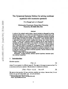
In this section we describe a globally convergent primal-dual NR algorithm with dynamic scaling parameter update that has the asymptotic 1.5-Q-superlinear rate of convergence. At each iteration the algorithm solves system (4.11). If the primal-dual direction (∆x, ∆λ) does not produce the superlinear reduction of the merit function, then the primal direction ∆x is used for minimization L(x, λ, k) in x. Therefore convergence to the neighborhood of the primal-dual solution is guaranteed by NR method (3.9)–(3.10). Eventually in the neighborhood of the primal-dual solution due to Theorem 1 one step of the PDNRD method (4.11) –(4.13) will be enough to obtain the desired 1.5-Q-superlinear reduction of the merit function and the bound (4.29) will take place. Figures 1 and 2 describe the PDNRD algorithm. It has some similarities to the globally convergent Newton’s method for unconstrained optimization when the Newton direction with steplength is used at each step to guarantee convergence. From some point on the steplength becomes equal one and “pure” Newton’s method converges with quadratic rate.

Step 1: Initialization: An initial primal approximation x0 ∈ IRn is given. An accuracy parameter ε > 0 and the initial scaling paramter k > 0 are given. Parameters α > 1, 0 < γ < 1, 0 < η < 0.5 σ > 0, θ > 0 are given. Set x := x0 , λ0 := (1, . . . , 1) ∈ IRm , r := ν(x, λ), λg := λ0 . Step 2: If r ≤ ε, Stop, Output: x, λ. Step 3: Find direction: (∆x, ∆λ) := P rimalDualDirection(x, λ). ˆ := λ + ∆λ. Set x ˆ := x + ∆x, λ ˆ ≤ min{r 23 −θ , 1 − θ}, Set x := x ˆ r := ν(x, λ), k := max{ √1 , k}, Goto Step 2. Step 4: If ν(ˆ x, λ) ˆ, λ := λ, r Step 5: Decrease t ≤ 1 until L(x + t∆x, λg , k) − L(x, λg , k) ≤ ηt(∇L(x, λg , k), ∆x) ˆ := λg ψ′ (kc(x + t∆x)). Step 6: Set x := x + t∆x, λ Step 7: If k∇x L(x, λg , k)k ≤

σ ˆ kλ k

− λg k, Goto Step 9.

Step 8: Find direction: (∆x, ∆λ) := P rimalDualDirection(x, λg ), Goto Step 5. ˆ ≤ γr, Set λ := λ, ˆ λg := λ, ˆ r := ν(x, λ), k := max{ √1 , k}, Goto Step 2. Step 9: If ν(x, λ) r Step 10: Set k := kα, Goto Step 8. Fig. 1. PDNRD algorithm.

20


function (∆x, ∆λ) := P rimalDualDirection(x, λ) begin ¯ := ψ′ (kc(x))λ λ Solve PDNR system:

 

∇2xx L(x, λ) +

1 I k2

−∇cT (x)

−kΨ ′′ (kc(x)) Λ∇c(x)

I

 

m where Ψ ′′ (kc(x)) = diag (ψ′′ (kci (x)))m i=1 , Λ = diag (λi )i=1

∆x ∆λ





=

−∇x L(x, λ) ¯−λ λ



,

end Fig. 2. Newton PDNRD direction.

The following lemma guarantees global convergence of the PDNRD method. Let us consider the iterative method 





s



 ∆x   −∇x L(x , λ)  = , Nk (xs , λ)      ¯ ∆λ λ−λ αs :

L(x + αs ∆x, λ, k) − L(x, λ, k) ≤ ηαs (∇L(x, λ, k), ∆x),

(5.1)

(5.2)

where 0 < η < 1.

xs+1 := xs + αs ∆xs .

(5.3)

We find the steplength αs from P. Wolfe’s condition [22]. Lemma 4. For any primal-dual pair (x, λ) ∈ / Ωε0 and fixed λ ∈ IRm ++ and k > 0 method (5.1)–(5.3) generates the primal-dual sequence that converges to the unconstrained minimizer of L(x, λ, k) in x. Proof. We can rewrite system (4.11) as follows. 1 ∇2xx L(xs , λ) + 2 In ) ∆xs − ∇c(xs )T ∆λ = −∇x L(xs , λ) = −∇x L(·), k

(5.4)

¯ − λ, −kΛΨ ′′ (kc(xs )) ∇c(xs )∆xs + ∆λ = λ

(5.5)

¯ = λΨ ′ (kc(xs )). where λ


⋆⋆

21

By substituting the value of ∆λ from (5.5) into (5.4) the primal Newton direction one can find from the following system ¯ = −∇x L(xs , λ, k), M (xs , λ, k)∆xs = −∇x L(xs , λ) where M (·) = M (xs , λ, k) = ∇2xx L(xs , λ) +

1 In − k∇cT (xs )Ψ ′′ (kc(xs )) Λ∇c(xs ). k2

Due to formula (4.4) the scaling parameter k > 0 increases unboundedly only when (x, λ) approaches ¯ the solution. It means there is a bound k¯ > 0 such that for any (x, λ) ∈ / Ωε0 the scaling parameter k ≤ k. Due to the convexity of f (x), concavity of ci (x),, transformation properties 40 , and the regularization term

1 k2 In

the matrix M (·) is positive definite with uniformly bounded condition number for all s, and

¯ i.e. k ≤ k,, m1 (x, x) ≤ (M (·)x, x) ≤ m2 (x, x)

, ∀x ∈ IRn

and 0 < m1 < m2 . It implies that ∆xs is a descent direction for minimization of L(x, λ, k) in x.. In addition if the steplength satisfies Wolfe’s condition we have lims→∞ k∇x L(xs , λ, k)k = 0 (see e.g.[22]). Therefore for any given (λ, k) ∈ IRm+1 ++ the sequence generated by method (5.1)–(5.3) converges to the unconstrained minimizer of L(x, λ, k) in x. Lemma 4 is proven. Combining the results of Proposition 1, Theorem 1 and Lemma 4 together we obtain the following. Theorem 2. Under the assumptions of Theorem 1 the PDNRD method generates the primal-dual sequence that converges to the primal-dual solution with asymptotic 1.5-Q-superlinear rate of convergence. The PDNRD algorithm uses the primal Newton direction with steplength and following the NR path until the primal-dual approximation reaches the neighborhood Ωε0 . Then due to Theorem 1 it requires at most O(log log ε−1 ) steps to find the primal-dual solution with accuracy ε > 0. The neighborhood Ωε0 is unknown a priori. Therefore the PDNRD may switch to Newton’s method for primal-dual system (4.5)-(4.6) prematurely, before (x, λ) reaches Ωε0 . Then PDNRD algorithm will recognize this in less than O(log log ε−1 ) steps and will continue following the NR trajectory with much bigger value of scaling parameter k > 0.

22


The algorithm has been implemented in MATLAB and tested on a variety of problems. The following section presents some numerical results from the testing.

6. Numerical results

Tables 1–12 present the performance of the PDNRD method on some problems from COPS [5] and CUTE [6] sets. In our calculations we use transformation ψq2 introduced in section 3. We show the number of variables n and constraints m. Then we show the objective function value, the norm of the gradient of the Lagrangian, the complementarity violation, the primal-dual infeasibility, and the number of Newton steps required to reduce the merit function by an order of magnitude. One of the most important observations following from the obtained numerical results is significant acceleration of convergence of the PDNRD method when the primal-dual sequence approaches the solution. It is in full correspondence with Theorem 1. For all problems we observed the “hot” start phenomenon: from some point on only one Newton step is required to reduce the value of the merit function at least by the order of magnitude. Table 1. CUTE, aircrfta: n = 5, m = 5, linear objective, quadratic constraints it

f

k∇L(x, λ)k

gap

constr violat

# of steps

0

4.031e+02

6.5281e+03

0.0000e+00

2.8370e+00

0

1

2.709e-07

6.1602e-02

1.8062e-07

3.7308e-05

4

2

3.974e-08

1.3987e-06

7.6025e-14

1.4923e-05

1

3

9.523e-16

1.7577e-10

2.6191e-20

9.2782e-11

1

Total number of Newton steps

6


⋆⋆

23

Table 2. CUTE, airport: n = 84, m = 210, linear objective, quadratic constraints it

f

k∇L(x, λ)k

gap

constr violat

# of steps

0

1.345e+07

1.6597e+06

3.4666e+02

1.0360e+02

0

1

4.801e+04

1.0268e+03

7.2841e+01

2.9730e-03

12

2

4.795e+04

2.2093e+00

1.3615e+00

3.0112e-07

13

3

4.795e+04

1.0899e-03

4.9758e-02

7.0738e-08

3

4

4.795e+04

3.9039e-05

1.0174e-03

2.6057e-09

2

5

4.795e+04

3.2575e-08

2.9585e-10

3.9753e-11

1

6

4.795e+04

7.1054e-12

5.5471e-14

1.7153e-14

1


32

Table 3. CUTE, avgasa: n = 6, m = 18, quadratic objective, linear constraints it

f

k∇L(x, λ)k

gap

constr violat

# of steps

0

-4.071e+00

4.4312e+00

9.0000e+00

-0.0000e+00

0

1

-4.175e+00

1.8651e-03

1.5612e-01

3.9168e-03

17

2

-4.169e+00

5.0646e-03

3.7190e-03

2.8939e-04

10

1

-4.169e+00

1.5713e-09

3.4780e-05

3.5657e-05

2

2

-4.169e+00

1.4853e-08

3.0974e-06

1.3140e-05

1

3

-4.169e+00

2.5863e-09

3.4712e-07

3.9769e-06

1

4

-4.169e+00

1.4468e-10

2.5983e-08

4.7697e-07

1

5

-4.169e+00

1.7776e-12

7.9031e-10

1.8035e-08

1

6

-4.169e+00

2.5008e-15

5.1032e-12

1.2809e-10

1

7

-4.169e+00

4.2327e-16

2.9326e-15

7.5273e-14

1


35

24

Igor Griva, Roman A. Polyak Table 4. COPS: Journal bearing: n = 5000, m = 5000, nonlinear objective, bounds it

f

k∇L(x, λ)k

gap

constr violat

# of steps

0

-4.504e+02

5.1364e+01

1.6229e+03

0.0000e+00

0

1

-8.002e-02

9.1922e-08

9.2602e-03

7.0564e-03

20

2

-1.550e-01

9.3995e-13

1.6896e-05

3.4093e-05

7

3

-1.550e-01

1.4592e-15

9.1966e-09

6.0043e-07

4

4

-1.550e-01

7.7398e-17

1.1702e-10

1.3002e-08

2

5

-1.550e-01

6.2450e-17

1.5082e-11

2.7984e-09

1

6

-1.550e-01

6.5919e-17

1.1229e-12

4.4897e-10

1

7

-1.550e-01

6.5919e-17

6.5135e-14

5.9776e-11

1

8

-1.550e-01

6.2450e-17

3.9621e-15

6.6580e-12

1


37

Table 5. CUTE: biggsb2: n = 1000, m = 1998, quadratic objective, bounds it

f

k∇L(x, λ)k

gap

constr violat

# of steps

0

-4.797e+00

3.1761e+01

8.9910e+02

-0.0000e+00

0

1

2.566e-02

9.8864e-02

1.7369e-05

7.6468e-04

12

2

1.500e-02

1.5879e-13

2.0104e-06

1.2438e-05

4

3

1.500e-02

3.3544e-14

3.1460e-07

2.6468e-06

1

4

1.500e-02

3.9262e-15

1.8169e-08

1.8039e-07

1

5

1.500e-02

4.4409e-16

1.2791e-10

1.3011e-09

1

6

1.500e-02

4.1517e-16

3.1744e-14

4.2613e-12

1


20


⋆⋆

25

Table 6. CUTE: congigmz: n = 3, m = 5, minimax: linear objective, nonlinear constraints it

f

k∇L(x, λ)k

gap

constr violat

# of steps

0

1.112e+04

8.5085e+03

3.6000e+01

1.4000e+01

0

1

3.321e+01

1.5855e+00

6.8324e+00

0.0000e+00

20

2

3.412e+01

6.5803e-03

7.5631e-01

1.4072e-01

7

3

2.800e+01

1.2877e-02

1.0537e-03

1.2996e-04

4

4

2.800e+01

3.9900e-07

2.8043e-05

1.5627e-06

2

5

2.800e+01

7.8753e-10

1.3920e-09

4.7149e-08

1

6

2.800e+01

1.9984e-15

3.9972e-13

1.0409e-11

1

7

2.800e+01

1.7764e-15

8.2580e-16

0.0000e+00

1


36

Table 7. CUTE: dtoc5: n = 998, m = 499, minimax: quadratic objective, quadratic constraints it

f

k∇L(x, λ)k

gap

constr violat

# of steps

0

5.020e+02

1.0020e+03

0.0000e+00

1.0020e+00

0

1

1.536e+00

6.5637e-07

2.3048e-03

1.1068e-04

5

2

1.535e+00

2.1110e-09

3.3520e-06

1.6171e-07

2

3

1.535e+00

4.7321e-13

3.3241e-07

1.6556e-09

1

4

1.535e+00

4.6872e-15

2.0525e-08

1.0679e-10

1

5

1.535e+00

1.1015e-15

8.4896e-10

4.7902e-12

1

6

1.535e+00

1.7208e-15

1.7808e-11

1.0170e-13

1

7

1.535e+00

1.2546e-15

5.4923e-14

4.2414e-16

1


12

26

Igor Griva, Roman A. Polyak Table 8. CUTE: gilbert: n = 1000, m = 1, quadratic objective, quadratic constraints it

f

k∇L(x, λ)k

gap

constr violat

# of steps

0

1.250e+10

1.5811e+08

0.0000e+00

5.0000e+04

0

1

4.821e+02

1.3971e-07

1.5065e+00

9.3099e-02

25

2

4.820e+02

9.2648e-07

1.3036e-01

7.4314e-03

5

3

4.820e+02

2.1307e-04

2.5920e-02

1.4683e-03

1

4

4.820e+02

1.5072e-05

3.0774e-03

1.7412e-04

1

5

4.820e+02

3.4087e-07

2.7104e-04

1.5334e-05

1

6

4.820e+02

1.8024e-10

3.6471e-08

9.9661e-07

1

7

4.820e+02

8.6531e-13

6.5325e-10

1.7851e-08

1

8

4.820e+02

5.5511e-16

1.5904e-12

4.3460e-11

1

9

4.820e+02

3.3307e-16

1.7876e-16

4.8850e-15

1


37

Table 9. Hock & Schittkowski 117: n = 15, m = 20, quadratic objective, quadratic constraints and bounds it

f

k∇L(x, λ)k

gap

constr violat

# of steps

0

5.436e+04

4.9754e+04

1.0800e+02

3.6000e+01

0

1

4.212e+02

7.6243e+00

9.6041e+00

5.5393e+00

62

2

3.235e+01

1.3047e-03

3.4444e-03

6.6456e-05

27

3

3.235e+01

3.2383e-07

1.5505e-04

8.0089e-06

2

4

3.235e+01

2.9211e-08

1.7757e-07

6.4741e-07

1

5

3.235e+01

2.2220e-11

8.2702e-10

5.5118e-09

1

6

3.235e+01

7.1054e-15

4.9593e-13

3.9804e-12

1


94


⋆⋆

27

Table 10. CUTE: optctrl6 n = 118, m = 80, quadratic objective, quadratic constraints it

f

k∇L(x, λ)k

gap

constr violat

# of steps

0

1.610e+06

2.4981e+06

1.5601e+06

9.8000e+00

0

1

1.937e+03

2.3443e-02

5.1348e+02

1.3507e-02

13

2

2.048e+03

9.4961e-09

8.8005e+01

1.5054e-03

12

3

2.048e+03

3.2521e-06

2.7358e+00

4.4311e-05

7

4

2.048e+03

2.4424e-08

4.6971e-01

7.5977e-06

2

5

2.048e+03

3.3227e-09

5.7014e-02

9.2203e-07

2

6

2.048e+03

3.6343e-09

4.8080e-03

7.7753e-08

2

7

2.048e+03

2.6724e-07

2.7814e-04

4.4978e-09

1

8

2.048e+03

2.5466e-11

5.3345e-09

1.7679e-10

1

9

2.048e+03

2.5580e-11

2.0977e-10

6.9508e-12

1

10

2.048e+03

2.7057e-11

8.2480e-12

2.7331e-13

1


42

Table 11. CUTE: optmass n = 126, m = 105, quadratic objective, linear and quadratic constraints it

f

k∇L(x, λ)k

gap

constr violat

# of steps

0

-9.642e-01

1.0025e+00

2.1000e+01

1.0000e-02

0

1

3.233e-02

2.8648e-06

2.7441e-01

8.1574e-03

91

2

-1.511e-01

1.3159e-04

6.6208e-03

9.0302e-04

25

3

-1.517e-01

2.8382e-05

4.6813e-04

5.9219e-05

7

4

-1.517e-01

7.2289e-09

1.0644e-05

2.7303e-05

1

5

-1.517e-01

3.0537e-11

3.5932e-07

1.5766e-06

1

6

-1.517e-01

1.1965e-12

7.8788e-09

8.6149e-09

1

7

-1.517e-01

2.0487e-15

5.0968e-11

2.6272e-12

1

8

-1.517e-01

5.5511e-17

2.5146e-14

1.3461e-15

1


128

28

Igor Griva, Roman A. Polyak Table 12. COPS: Isometrization of α -pinene n = 4000, m = 4000, nonlinear objective, nonlinear constraints it

f

k∇L(x, λ)k

gap

constr violat

# of steps

0

1.096e+10

9.6378e+10

0.0000e+00

2.3600e+01

0

1

2.095e+01

6.1850e-04

2.6426e+00

4.1064e-05

17

2

1.989e+01

1.0998e-01

2.5621e-01

2.8963e-06

4

3

1.987e+01

2.9277e+00

1.6708e-02

2.4864e-07

2

4

1.987e+01

3.0175e-04

9.4867e-04

2.1777e-08

2

1

1.987e+01

1.2649e-03

2.1393e-06

1.3047e-09

1

2

1.987e+01

4.4104e-06

1.1108e-07

7.1941e-11

1

3

1.987e+01

1.4076e-08

5.5255e-09

3.6255e-12

1

4

1.987e+01

1.5019e-09

2.5360e-10

1.6685e-13

1


29


⋆⋆

29

7. Concluding remarks

Theoretical and numerical results obtained for the PDNRD method emphasize the fundamental difference between the primal-dual NR approach and Newton NR methods [19], [26], which are based on sequential unconstrained minimization L(x, λ, k) followed by the Lagrange multipliers update. The Newton NR method converges globally with a fixed scaling parameter, keeps stable the Newton area for the unconstrained minimization and allows the observation of the “hot start” phenomenon [19], [24]. It leads to asymptotic linear convergence with a given factor 0 < γ < 1 in one Newton step. However, the unbounded increase of the scaling parameter compromises convergence, since the Newton area for unconstrained minimization shrinks to a point. Moreover, in the framework of the NR method, any drastic increase of the scaling parameter after the Lagrange multipliers update leads to a substantial increase of the computational work per update because several Newton steps are required to get back to the NR trajectory. The situation is fundamentally different with Newton’s method for the primal-dual system (4.5)-(4.6) in the neighborhood of Ωε0 . The drastic increase of the scaling parameter does not increase the computational work per step. Just the opposite: by using (4.13) for the scaling parameter update we obtain the Newton direction for the primal-dual system (4.5)-(4.6) close to the Newton direction for the Lagrange system of equations that corresponds to the active set. The latter direction guarantees the quadratic convergence of the corresponding primal-dual sequences ([23]). Therefore the PDNRD uses the best properties of both Newton’s NR method far from the solution and Newton’s method for the primal-dual system (4.5)-(4.6) in the neighborhood of the solution. At the same time PDNRD is free from their fundamental drawbacks. The PDNRD method recalls the situation in unconstrained smooth optimization, in which Newton’s method with steplength is used to guarantee global convergence. Locally the steplength automatically becomes equal one and Newton’s method gains the asymptotic quadratic convergence. A few important issues remain for future research. The NR multipliers method with inverse proportional scaling parameter update [28] generates such a primal-dual sequence that the Lagrange multipliers corresponding to the inactive constraints converge quadratically to zero. This fact can be used to eliminate the inactive constraints in the early stage of the computational process. Then the PDNRD method

30


evolves into Newton’s method for the Lagrange system of equations that corresponds to the active constraints. Therefore under the standard second order optimality conditions, the PDNRD method has a potential to be augmented to a globally convergent method with asymptotic quadratic rate. Another important issue is the generalization of the PDNRD method for nonconvex problems. Also, more work should be done to find an efficient way of solving the PD system (4.11) that accounts for the system’s special structure.

Acknowledgements. We thank the anonymous referees for their valuable remarks, which contributed to improvement of the paper. Also, we are thankful to Michael Lulis for careful reading the manuscript and fruitful discussions.

References 1. A. Auslender, R. Comminetti, M. Haddou Asymptotic analysis of penalty and barrier methods in convex and linear programming, Mathematics of Operations Research 22, (1997), 43–62. 2. M. Bendsoe, A. Ben-Tal, J. Zowe (1994): Optimization Methods for Truss Geometry and Topology Design, Structural Optimization 7, 141–159 3. A. Ben-Tal, I. Yuzefovich and M. Zibulevski (1992): Penalty/Barrier Multiplier Method for minimax and constrained smooth convex problems, Research Report 9/92, Optimization Laboratory, Faculty of Industrial Engineering and Management, Technion 4. A. Ben-Tal, M. Zibulevski (1997): Penalty-barrier methods for convex programming problems, SIAM Journal on Optimization, 7, 347–366 5. A.S. Bondarenko, D.M. Bortz, J.J. More (1999): COPS: Large-scale nonlinearly constrained optimization problems, Mathematics and Computer Science Division, Argonne National Laboratory, Technical Report ANL/MCS-TM-237 6. I.

Bongartz,

A.R.

Conn,

N.

Gould,

Ph.L.

Toint,

Constrained

and

unconstrained

testing

environment,

www.cse.clrc.ac.uk/Activity/CUTE+74 7. M. Breitfelt, D. Shanno (1996): Experience with modified log-barrier method for nonlinear programming, Annals of Operations Research, 62, 439–464 8. R. Cominetti and J.-P. Dussault (1994): A stable exponential-penalty algorithm with superlinear convergence, Journal of Optimization Theory and Applications, 83 9. J.-P. Dussault (1998): Augmented penalty algorithms, I.M.A. Journal on Numerical Analysis, 18, 355-372 10. A. Forsgren, P. Gill (1998): Primal-dual interior methods for nonconvex nonlinear programming, SIAM Journal on Optimization 8, 1132–1152 11. D. M. Gay and M. L. Overton and M. H. Wright (1998): A primal-dual interior method for nonconvex nonlinear programming, A primal-dual interior method for nonconvex nonlinear programming, Advances in Nonlinear Programming, Ed. Y. Yuan, 31–56, Kluwer Academic Publishers, Dordrecht.


⋆⋆

31

12. N.I.M. Gould (1986): On the accurate determination of search directions for simple differentiable penalty functions, I.M.A. Journal on Numerical Analysis, 6, 357–372 13. N.I.M. Gould (1989): On the convergence of a sequential penalty function method for constrained minimization, SIAM Journal on Numerical Analysis, 26, 107–108 14. N.I.M. Gould, D. Orban, A. Sartenaer, and P. Toint (2001): Superlinear convergence of primal-dual interior point algorithms for nonlinear programming, SIAM Journal on Optimization, 11, 974–1002 15. B.W. Kort, D.P. Bertsekas (1973): Multiplier methods for convex programming, Proceedings, IEEE Conference on Decision and Control, San Diego, California, 428–432 16. I. Lustig, R. Marsten, D. Shanno (1994): Computational experience with globally convergent primal-dual predictorcorrector algorithm for linear programming, Mathematical Programming 66, 23–135 17. N. Megiddo (1989): Pathways to the optimal set in linear programming, in N. Megiddo, ed., Interior Point and Related Methods, Springer-Verlag, New York , Ch. 8, 131–158 18. S. Mehrotra (1992): On implementation of a primal-dual interior point method, SIAM Journal on Optimization 2, 575–601. 19. A. Melman, R. Polyak (1996), The Newton Modified Barrier Method for QP Problems, Annals of Operations Research, 62, 465–519 20. S. Nash, R. Polyak and A. Sofer (1994): A numerical comparison of Barrier and Modified Barrier Method for LargeScale Bound-Constrained Optimization, in ”Large Scale Optimization, state of the art”, Ed. by W. Hager, D. Hearn and P. Pardalos, Kluwer Academic Publisher , 319–338 21. E. Ng, B.W. Peyton (1993): Block sparse Cholesky algorithms on advanced uniprocessor computers, SIAM Journal of Scientific Computing, 14, 1034–1056 22. J. Nocedal, S. Wright (1999): Numerical Optimization, Springer, New York 23. B.T. Polyak (1970): Iterative methods for optimization problems with equality constraints using Lagrange multipliers, Journal of computational mathematics and mathematical physics, 10, 1098–1106 24. R. Polyak (1992): Modified Barrier Functions Theory and Methods, Mathematical Programming 54, 177–222 25. R. Polyak, M. Teboulle (1997): Nonlinear Rescaling and Proximal-like Methods in convex optimization, Mathematical Programming 76, 265–284 26. R. Polyak, I. Griva, J. Sobieski (1998): The Newton Log-Sigmoid method in Constrained Optimization, A Collection of Technical Papers, 7th AIAA/USAF/NASA/ISSMO Symposium on Multidisciplinary Analysis and Optimization 3, 2193–2201 27. R. Polyak (2001): Log-Sigmoid Multipliers Method in Constrained Optimization, Annals of Operations Research 101, 427–460 28. R. Polyak (2002): Nonlinear rescaling vs. smoothing technique in convex optimization, Mathematical Programming 92, 197–235 29. R. Polyak, I. Griva, Primal-Dual Nonlinear Rescaling method for convex optimization, Techncal Report 2002-05-01, George Mason University, to appear in JOTA in July 2004, (http://mason.gmu.edu/ rpolyak/papers.html).

32

Title Suppressed Due to Excessive Length – supply \combirunning

30. D. Shanno, R. Vanderbei (1999): An interior-point algorithm for nonconvex nonlinear programming, COAP 13, 231–252 31. R. Vanderbei (1995): Symmetric Quasidefinite Matrices SIAM Journal on Optimization, 5, 100–113 32. S. Wright (1997): Primal-Dual Interior Points methods, SIAM 33. Y. Zhang (1996): Solving Large-Scale Linear Programs by Interior-Point Methods Under MATLAB Environment, Dept. of Computational and Applied Mathmatics, Rice University, Houston 34. Y. Zhang, R. Tapia, J. Dennis (1992): On the superlinear and quadratic convergence at primal-dual interior point linear programming algorithms, SIAM Journal on Optimization 2, 304–324

Primal-dual nonlinear rescaling method with

Primal-dual nonlinear rescaling method with

Suggest Documents

Nonlinear Rescaling as Interior Quadratic Prox ... - Semantic Scholar

Numerical analysis of the rescaling method for parabolic problems ...

Racialization and Rescaling - Tulane University

Newton-Raphson Method Nonlinear Equations

Rescaling of aerial survey data with information ... - Wiley Online Library

Accelerated rescaling of single Monte Carlo simulation runs with the ...

The Dynamical Systems Method for solving nonlinear equations with ...

A nonintrusive method to approximate linear systems with nonlinear ...

A new algorithm of nonlinear conjugate gradient method with ... - SciELO

Modified LQP Method with a New Search Direction for Nonlinear

Nonlinear Projection with the Isotop Method - UniversitÃ© catholique de ...

adaptive nonlinear filtering with the support vector method - eurasip

Inexact Newton's method to nonlinear functions with ... - CiteSeerX

An Asymptotic Method with Applications to Nonlinear Coupled Partial ...

A nonintrusive method to approximate linear systems with nonlinear

A nonlinear second derivative method with a variable ...

an iterative method for solving nonlinear least squares problems with ...

Adomian Decomposition Method for a Nonlinear Heat Equation with

Image Prediction Method with Nonlinear Control Lines Derived from ...

Nonlinear silicon photonics analyzed with the moment method

A Primal-Dual Interior-Point Method for Nonlinear Programming with ...

Canonical sampling through velocity-rescaling

An Adaptive Kalman Filter with Dynamic Rescaling of Process Noise

Accelerated rescaling of single Monte Carlo simulation runs with the ...