170
IEEE/ACM TRANSACTIONS ON NETWORKING, VOL. 19, NO. 1, FEBRUARY 2011
Primary User Activity Modeling Using First-Difference Filter Clustering and Correlation in Cognitive Radio Networks Berk Canberk, Student Member, IEEE, Ian F. Akyildiz, Fellow, IEEE, Fellow, ACM, and Sema Oktug, Member, IEEE
Abstract—In many recent studies on cognitive radio (CR) networks, the primary user activity is assumed to follow the Poisson traffic model with exponentially distributed interarrivals. The Poisson modeling may lead to cases where primary user activities are modeled as smooth and burst-free traffic. As a result, this may cause the cognitive radio users to miss some available but unutilized spectrum, leading to lower throughput and high false-alarm probabilities. The main contribution of this paper is to propose a novel model to parametrize the primary user traffic in a more efficient and accurate way in order to overcome the drawbacks of the Poisson modeling. The proposed model makes this possible by arranging the first-difference filtered and correlated primary user data into clusters. In this paper, a new metric called the Primary User Activity Index, , is introduced, which accounts for the relation between the cluster filter output and correlation statistics. The performance of the proposed model is evaluated by means of traffic estimation accuracy, false-alarm probabilities while keeping the detection probability of primary users at a constant value. Simulation results show that the appropriate selection of the Primary User Activity Index, higher primary-user detection accuracy, reduced false-alarm probabilities, and higher throughput can be achieved by the proposed model.
8
Index Terms—Clustering, cognitive radio (CR) networks, primary user activity modeling.
I. INTRODUCTION
I
N COGNITIVE radio (CR) networks, primary users (PUs) are defined as wireless devices that have the license to operate in a specific spectrum band. Since PUs have priority to utilize the licensed spectrum, their communication should not be interrupted or interfered with any other users. However, CR users are supposed to sense the spectrum and utilize the unused
Manuscript received December 31, 2008; revised December 20, 2009; accepted June 20, 2010; approved by IEEE/ACM TRANSACTIONS ON NETWORKING Editor M. Buddhikot. Date of publication August 19, 2010; date of current version February 18, 2011. This work was supported by the Istanbul Chamber of Industry (ISO). The work of I. F. Akyildiz was supported by the U.S. National Science of Foundation under Award CNS-0721580. B. Canberk was with the Broadband Wireless Networking Laboratory (BWNLab), School of Electrical and Computer Engineering, Georgia Institute of Technology, Atlanta, GA 30332 USA. He is now with the Department of Computer Engineering, Faculty of Electrical and Electronic Engineering, Istanbul Technical University, 34469 Istanbul, Turkey (e-mail:
[email protected]). I. F. Akyildiz is with the Broadband Wireless Networking Laboratory (BWNLab), School of Electrical and Computer Engineering, Georgia Institute of Technology, Atlanta, GA 30332 USA (e-mail:
[email protected]). S. Oktug is with the Department of Computer Engineering, Faculty of Electrical and Electronic Engineering, Istanbul Technical University, 34469 Istanbul, Turkey (e-mail:
[email protected]). Digital Object Identifier 10.1109/TNET.2010.2065031
bands in an opportunistic manner. CR users may occupy available bands as long as the corresponding PU is active, but must immediately evacuate the band as soon as the corresponding PU appears [1]. CR users should intelligently determine the ongoing PU activities in a licensed spectrum band to avoid interference with the PUs [1]. Moreover, the PU activities need to be accurately modeled so that CR users can evacuate the band without affecting PU activities. CR users also need to detect spectrum holes to identify transmission opportunities so that the spectrum usage is maximized [2]. Hence, it could be stated that precise estimations/modeling of PU activities leads to much more effective spectrum usage for CR users. In recent studies, the PU activity is assumed to follow the Poisson model [3]–[6]. However, the Poisson model fails in capturing the bursty and spiky characteristics of the monitored data [2], [7], [8]. As a result, the existing works based on the Poisson model consider the PU activities as smooth and burstfree, in which short-term fluctuations are neglected. Moreover, some large-scale measurement-driven characterizations of the PU activities in cellular networks are also carried out for different spectrum bands. In [9], the authors analyze the spectrum occupancy of PUs in GSM and UMTS bands. In [10], the PU activities are analyzed in the New York cellular bands, i.e., CDMA and GSM. In [11], the authors analyze the call logs of a switch of a cellular GSM provider in Qingdao, China. In [2], it is pointed out that the PU activity durations are nonexponential and changes in time scale violating the Poisson assumptions. It was also pointed out that the spectrum usage of PUs fluctuates significantly even with a few seconds, hence CR users must be aware of these short-term fluctuations. Note that the PU activity models in that work are based on long-term observations. Overall, the Poisson model approximates the PU activities as smooth and burst-free traffic. Though the PU activity exhibits short-term temporal diversity, i.e., significant and spiky fluctuations over time, these variations are not captured by the Poisson model, as shown in Fig. 1. The model represents the ON period, i.e., the active transmission duration of a PU, by the horizontal dBm. The OFF period, which level at constant amplitude of represents the absence of PU activity, is also given by the condBm. It could be observed that the actual stant amplitude of PU activity fluctuates during the ON period, which is not exactly tracked by the Poisson model. Some of these fluctuations result in durations, where the PU is actually absent, shown by the dashed lines. These durations, which are classified as a part of the ON period by the Poisson model, cause missed transmission
1063-6692/$26.00 © 2010 IEEE
CANBERK et al.: PU ACTIVITY MODELING USING FIRST-DIFFERENCE FILTER CLUSTERING AND CORRELATION IN CR NETWORKS
171
Fig. 1. Missed transmission opportunities caused by the Poisson modeling.
opportunities for the CR users. The Poisson model is incapable of identifying fluctuations. This leads to fewer cases of correct spectrum hole detection, thus causing a degradation in CR network performance. In this paper, we introduce a novel PU activity model addressing the potential drawbacks of the Poisson modeling with the following contributions. • A new PU activity detection technique based on the FirstDifference Clustering scheme is introduced. • A new temporal correlation-based PU activity modeling scheme in order to detect the spectrum holes in a band is proposed. • The PU activity detection and the spectrum hole detection schemes are combined to maximize the CR network performance. In this work, spiky and bursty PU activities are captured more accurately. Moreover, a new parameter called the Primary User Activity Index (the PU activity index), , is introduced to parametrize the PU activities as well as the spectrum holes. Finally, the overall CR network performance, in terms of estimation accuracy, false-alarm probabilities, and throughput is evaluated under different -values. The rest of the paper is organized as follows. In Section II, the overview of the network architecture and the model we proposed are described. In Section III, we explain the ClusteringModeling Module by giving details of the proposed PU activity modeling. In Section IV, the performance of the proposed model is evaluated in terms of traffic estimation, false-alarm probabilities, and throughput. In Section V, we conclude the paper by summarizing the achievements and giving future directions.
Fig. 2. Block diagram of the proposed model.
TABLE I KEY NOTATIONS
The model we propose consists of two main modules: the PU Activity Monitoring Module and the Clustering-Modeling Module, which are illustrated in Fig. 2. The notations used are listed in Table I. The PU Activity Monitoring Module, which is implemented in each CR user, monitors the spectrum band and samples the PU activity. We use the following noncooperative spectrum sensing scheme at each CR user [3], [12]: (1) where is the th sample of the monitored PU activity and vector , which is sampled at the sampling frequency defined as (2)
II. NETWORK ARCHITECTURE AND PROPOSED MODEL We consider an infrastructure-based CR network architecture integrated in a PU network that has the license to operate in a certain spectrum band [4]. Moreover, the CR network has a centralized network entity such as a base station and associated CR users. Each CR user monitors the spectrum band and sends its local observations, i.e., the monitored PU activities, to the base station, which broadcasts the PU activity model to the CR users.
where is the total number of PU monitored activity samples. and in (1) are the hypotheses that indicate eiMoreover, ther the PU does not have an activity or does have an activity in (1) repin the spectrum band, respectively. In addition, resents the additive white Gaussian noise (AWGN) with zero , and is the primary mean and variance user’s unknown signal, which is an independent and identically and variance distributed (iid) random process with mean as in [13]. It is also assumed that and
172
IEEE/ACM TRANSACTIONS ON NETWORKING, VOL. 19, NO. 1, FEBRUARY 2011
are independent. Thus, the signal-to-noise ratio (SNR) is . given by Once the monitoring is finished, the PU Activity Monitoring Module gives the monitored PU activity vector for modeling and analysis to the Clustering-Modeling Module, which is implemented in the base station. The Clustering-Modeling Module activates its Clustering Engine, where the monitored PU activity samples are accumulated into clusters using a first-difference filtering procedure enhanced with temporal correlation. As a result, a new PU activity vector with clusters is generated and then input to the Modeling Engine as seen in Fig. 2. In this engine, a correlation-based modeling scheme produces the new modeled PU activity and parametrizes PU activity characteris, the probability of PU absence, and tics, i.e., producing , the probability of PU presence. The details of the Clustering-Modeling Module are given in Section III. The newly generated PU activity characteristics and the modeled PU activity vector are fed back to the CR user. Here, the modeled PU activity is input to the energy detector to be used for spectrum sensing. Since the energy detector gets samples of iterations. At the end size , it completes the operation in of the operation, the energy detector triggers the PU Activity Monitoring Module using the local clock for a new analysis. In the model, we use the maximum a posteriori (MAP) energy detection, i.e., the a posteriori PU activity probabilities, which could be summarized as follows [3], [13]. The energy detector consists of a bandpass filter, a squaring module, an integrator, and a decision maker. The energy of the received signal is bandpassed by the filter with bandwidth . The output signal of this bandpass filter is squared and integrated over the sensing time . The output of the integrator is compared to a threshold in the decision maker to decide whether the PU is present or not. The output of the integrator follows the chi-square distribution [13]. When the number of samples is large, the output can be approximated by Gaussian distribution using central limit and the theorem [14]. Therefore, the false-alarm probability can be evaluated by considering PU acdetection probability tivity characteristics as [3]
(3)
(4) is the th sample of , which is the modeled PU acwhere gives the tivity vector , which is smaller than or equal to number of samples; is the sensing time; is the complete is the incomplete Gamma function; Gamma function; is the generalized Marcum Q-function. and Moreover, the proposed model calculates the maximum achievable throughput of a CR user as in [15] (5) where is the total frame duration, and throughput of a CR user without PU existence.
is the is equal to
Fig. 3. Flowchart of the clustering engine.
and
, where is the received power of the CR user is the noise power. III. CLUSTERING-MODELING MODULE
The Clustering-Modeling Module has two engines to process the monitored PU activity: the Clustering Engine and the Modeling Engine, as shown in Fig. 2. The details of the engines are explained. A. Clustering Engine The Clustering Engine works based on the flow diagram given in Fig. 3. When the PU Activity Monitoring Module gives the monitored PU activity vector to the Clustering-Modeling Module, it activates its Clustering Engine. Here, the monitored PU activity samples are accumulated into clusters. A cluster is a vector where PU activity samples are accumulated according to some to express the hypothesis tests. We introduce the notation th cluster. In a cluster , the PU samples are assumed to be homogeneous. We exploit this homogeneity for more accurate detection of PU activities. Since all samples in the th cluster have same power level, the energy detector, shown in Fig. 2, results with the same decision for them, leading to a more accurate detection as long as the samples within a cluster are highly correlated. In this engine, the monitored PU activity samples are clustered using a first-difference filtering procedure enhanced with temporal correlation. The details of the first-difference filtering are given in Appendix A. As a result, a new PU activity vector with clusters is generated and then input to the Modeling Engine. At the beginning of the clustering process, the Clustering Engine receives the monitored PU activity vector from the PU Activity Monitoring Module and sets , indicating the
CANBERK et al.: PU ACTIVITY MODELING USING FIRST-DIFFERENCE FILTER CLUSTERING AND CORRELATION IN CR NETWORKS
start index of the monitored PU activity vector; the cluster index , representing the first cluster; and the randomly predeter, the clustering parameter (detailed in mined parameters Appendix A), and , the correlation parameter (detailed in . Since the monitored PU activity Appendix B), for is input to the Clustering Engine Module, we may assume that the modeled PU activity vector is identical to the monitored . PU activity vector input to the Clustering Engine, i.e., and Then, all the consecutive samples (the current sample ) are passed through the first-difference the last sample finite-impulse response (FIR) filter [detailed in Appendix A and is calculated in (38)]. In the next step, the filter output checked with a -test (detailed in Appendix A). If the -test is successful, the -test (detailed in Appendix B) is applied. Conis placed in the sequently, the modeled PU activity sample existing cluster with its predecessor if both tests are successful, whereas any fail from these two tests leads to form a new cluster . This process the sample is repeated until all the samples in the monitored PU activity vector are analyzed. Then, the clustered PU activity vector of size is formed by mean values of each cluster. , which As a result, only the modeled PU activity sample (successful in -test) and is close to its predecessor highly correlated with the last two samples , (successful in -test), is placed in the same cluster with its pre. By using clustering, groups of first-differdecessor ence filtered PU activity samples that have different correlation statistics are separated. In other words, spiky and bursty characteristics of the modeled PU activity are more accurately distinguished by employing clustering, which leads the CR user to detect the PU activity fluctuations more precisely, hence causing less interference. B. Modeling Engine The Modeling Engine produces a correlation-based modeling scheme in order to parametrize the PU activity characteristics. The operations performed in this engine have a flow diagram shown in Fig. 4. At the Modeling Engine, and are set to 1 and the is . After this preprocessing, randomly predetermined for the Modeling Engine enters the loop until all samples are executed. At each run, the engine determines a decision region among using Table III for the pair of clusters four regions. Decision regions are defined for a pair of clusters , and each pair can reach only one of the regions at the end of the Modeling Engine. Moreover, the regions are expressed by different combinations of the two binary variables and , which are defined in Table II. The two binary variables and are employed to mathematically express the -test [detailed in Appendix A and given in (47)] and the correlation slope test [detailed in Appendix B and given in (50)], respectively. More precisely, the variables and take the value 1 under a certain hypothesis, and 0 if the hypothesis is not true. These variables and their hypotheses are expressed in Table II. represents that the -test As seen in Table II, the variable in (47), which is realized in the Modeling Engine, is successful . The , which is the complement of , represents that the -test in (47) failed. Moreover, the
173
Fig. 4. Flowchart of the modeling engine.
TABLE II
VARIABLES
9, AND THEIR HYPOTHESES
in Table II is used when the correlation slope variable test, calculated in the Modeling Engine using (50), is positive . The
, which is the complementary
of , shows that the result of (50) is negative. At each decision region, there are two possible decisions that and can take. These are and the clusters . means that the clusters are modeled as the absence of PU activity, whereas indicates that the clusters are modeled as the existence of PU activity. The regions, their mathematical expressions, and the decisions for the cluster at each region are shown in Table III. pair In addition, the interpretation of each decision region for the is illustrated in Fig. 5. Note that cluster pair the threshold value in Fig. 5 is selected as the mean power of the monitored PU activity, and is the cluster index.
174
IEEE/ACM TRANSACTIONS ON NETWORKING, VOL. 19, NO. 1, FEBRUARY 2011
Fig. 5. Interpretation of decision regions.
TABLE III DECISION REGIONS
and , as well as the calculated values of and are input to the PU Activity Monitoring Module as seen in Fig. 2. Using the Modeling Engine, we analyze each cluster pair independently, thus the fluctuations in PU activity are better classified. This leads to more accurate detection of the transmission opportunities and an increase in the CR network performance. The calculations performed at the end of the Modeling Engine are explained as follows. . This 1) We first define the Primary User Activity Index metric is defined to parametrize the relation between the vector of the clustering parameters defined in (41) and the vector of the correlation parameters defined in (46). It is expressed as follows: (6) By substituting (41) and (46) into (6), the Primary User Activity Index can be calculated as follows:
Each region, which indicates the decision of being BUSY and , is described using IDLE for a pair of clusters Table III and Fig. 5 as follows. has a decreasing • Region 1: Since the pair , has a higher power amplitude than slope . Moreover, they are not highly correlated , thus they are not close to each other, indicating that they have different decisions. Consequently, merging the two results , we state that is BUSY because of its higher is IDLE because it is not close power level, and to . has a decreasing • Region 2: Since the pair , has a higher power amplitude than slope . Moreover, they are highly correlated , thus they are close enough to each other, indicating that they have identical decisions. Consequently, merging the two results , we state that is IDLE because of its higher is IDLE as well because it is power level, and close to . has an increasing • Region 3: Since the pair , has a higher power amplitude than slope . Moreover, they are not highly correlated , thus they are not close to each other, indicating that they have different decisions. Consequently, merging the two results , we state that is BUSY because of its higher is IDLE because it is not close to power level, and . has an increasing • Region 4: Since the pair , has a higher power amplitude than slope . Moreover, they are highly correlated , thus they are close enough to each other, indicating that they have identical decisions. Consequently, merging the two results , we state that is BUSY because of its higher is BUSY as well because it is close power level, and to . As the output of the Modeling Engine, the total number of , the total number of BUSY clusters , IDLE clusters the modeled PU activity vector , PU activity characteristics
(7) By substituting (40) and (45) into (7), we obtain
as
(8) Therefore, the PU Activity Index vector using (44) as follows:
is generated
(9) where is the number of monitored PU activity samples. The first term in (8) indicates that represents the clustering effect, whereas the second term shows that also accounts for the correlation captures both the clustering and effect. Therefore, correlation effects. In the evaluations, we analyze the clustering and correlation effects of the PU activity index separately. More detailed explanation about separate analysis of clustering and correlation effects using the PU activity index is provided in Section IV. The sampling errors will affect our PU activity index calculation and the Poisson assumption similarly, thus we can assume the same sampling errors for both cases. 2) The number of clusters considered as BUSY at any th , is calculated using the decision regions in run, Table III as (10)
CANBERK et al.: PU ACTIVITY MODELING USING FIRST-DIFFERENCE FILTER CLUSTERING AND CORRELATION IN CR NETWORKS
where is the number of monitored PU activity samples. This three-term equation can be retrieved from the flow diagram given in Fig. 4 by following logical paths to reach regions 4, 1, and 3, which are defined in Table III, respectively. They are combined by the logical expression since a pair of clusters can reside only in one of the three available regions. in the first term of (10) shows that . Besides, and are highly correlated because of . Since these two variables are highly correlated in an increasing relationship, they are both considered as BUSY at region 4 (the number 2 in the first term). Therefore, the result is . Looking at the second term of (10), one can and are in a decreasing trend , see that , hence and they are not highly correlated is IDLE whereas is BUSY at region 1. Therefore, . The third term of (10) indithe result is and are in an increasing relacates that and they are not highly correlated , thus tionship is BUSY and is IDLE at region 3. As a re. sult, 3) The number of clusters considered as IDLE at any th , is calculated using the decision regions in run, Table III as
(IDLE or BUSY) the two clusters have. By considering only two clusters, the model achieves more accurate detection of the PU activity, thus possible fluctuations and missed transmission opportunities are better captured. As an example, consider the case when the two clusters have as seen in Table II) but they an increasing slope ( as seen in Table II). are not highly correlated ( By replacing and in (12), we obtain . After some Boolean aland in (12) gebra calculation steps, , which is calculated in (12) is expressed in terms of as (14) and
(15) Therefore, The total number of clusters considered as IDLE is calculated using (14) as (16)
(11) This three-term equation can also be retrieved from the flow diagram given in Fig. 4 by following the logical paths to reach regions 2, 1, and 3, which are defined in Table III, respectively. Using the decision regions in Table III, we see in regions 1 and 3, whereas in that region 2. 4) Using (10) and (11), we derive a mathematical expression in terms of for the modeled PU activity at , and as follows. In (10), we observe that the first term represents that both clusters are BUSY. Similarly, in (11), the first term strictly indicates that both clusters are IDLE. Therefore, these first terms of (10) and (11) are used to express the cases where both clusters have identical characteristics. The second and the third terms in (10) and (11) identify that the two clusters have opposite characteristics, thus they are utilized to express the cases where one cluster is BUSY and the other one is IDLE. After neglecting constant values in the first term of (10) and (11), the modeled PU activity is defined as
Similarly, the total number of clusters considered as BUSY is expressed using (15) as (17) 7) Furthermore, we define the modeled PU activity characteristics, i.e., the probability of IDLE and BUSY periods, and as (18) and (19) The total number of IDLE and BUSY periods is , hence in (18) and in (19) become
(12) where is the number of monitored PU activity samples. 5) The modeled PU activity is calculated using (12) as
175
(20) and
(13) 6) The calculated in (12) shows the behavior of the clusters. In other words, indicates what characteristics
(21)
176
IEEE/ACM TRANSACTIONS ON NETWORKING, VOL. 19, NO. 1, FEBRUARY 2011
8) Using (20) and (21), the modeled PU activity characterisand are expressed as tics
(22) and
Fig. 6. Network topology.
(23) 9) After obtaining the PU activity characteristics, i.e., in (22) and in (23), we can reformulate the CR-spein cific parameters, i.e., the probability of false alarm (3) and the CR user’s achievable throughput in (5) as follows. defined in (22) into (3), we obtain By substituting as (24) Similarly, by substituting defined in (22) into (5), we define the CR user’s achievable throughput as in [15]
(25) where in (24) and (25) is the number of monitored PU activity samples. IV. PERFORMANCE EVALUATION The performance of the proposed PU activity model is compared to the Poisson PU activity model under different conditions, estimation accuracy, false alarm probabilities, and CR User achievable throughput. The simulation environment and these different evaluations are presented. A. Simulation Environment Both system modules are implemented in MATLAB environment. In the evaluations, we use a network topology shown in Fig. 6, where we consider a centralized PU network operating MHz in a licensed spectrum band with a bandwidth of [15]. This PU network consists of one PU and one primary base station. The primary base station has a PU transmission range m [16] as shown in Fig. 6. The PU, which has an unof known traffic pattern, communicates with the primary base station in this range [13]. Moreover, we consider a CR network that operates within the PU transmission range in an opportunistic
manner. This CR network has one CR base station and 20 CR users that are spread out within the PU transmission range as shown in Fig. 6. The reason to select 20 CR users is explained as follows. In our simulations, we adopt a noncooperative spectrum sensing scheme at each CR user, as defined in Section II. The CR users only send their monitored data to the base station, and they do not exchange their monitored PU activity data with each other. Therefore, we analyze that the increase of the CR users within the PU transmission range does not have a significant effect on the PU activity monitored by each CR user. Consequently, we evaluate the system performance with a fixed number of CR users, which is selected as 20. In the CR network, each CR user monitors the PU’s spectrum samples of PU activity with band for 10 s and takes MHz [15]. We prefer taking 10 s of a sampling frequency spectrum monitoring in order to capture PU activity’s short-term temporal variations and fluctuations [2]. Since the CR network has 20 CR users, the simulation is run with 20 replications (local clock triggers the PU activity Monitoring Module 20 times as seen in Fig. 2), and the confidence intervals are shown in the figures whenever they are not negligible. In addition, the frame ms, and the duration in the CR network is fixed at , energy detector exploits a maximum vector size of where ms ms. Besides, the SNR value for the in (1) is assumed to be dB since low-SNR hypothesis regime is considered for CR network. The fading effects will be the same for both the Poisson model and our proposed model because CR users are stable. In addition, the PU is protected with a given target probability of detection 0.9, and the CR user under hypothesis is constant with dB. transmission The detection threshold in (4) is regulated according to the target detection probability in (4), i.e., the energy detector is while calculating the threshold trained with from 0 to in (4), to reach the target probability of detection [15]. In order to evaluate the effects of the clustering and the correlation parameters on the proposed model separately, two different PU activity indexes are introduced using (7). More precisely, the clustering effect is analyzed by the PU activity index , whereas the correlation effect is observed using .
CANBERK et al.: PU ACTIVITY MODELING USING FIRST-DIFFERENCE FILTER CLUSTERING AND CORRELATION IN CR NETWORKS
and , which are both derived from (7), are explained in detail as follows. , the correlation • In the case of the clustering effect parameter in (7) is selected by trial as 0.5 for all . The performance of the proposed model for is evaluated by varying the clustering parameter in (7). Thus, (7) becomes all (26) By substituting (40) into (26), we express follows:
as
As seen in (29) derived by (7), the clustering parameter for all does not have an additional since is kept constant at 0.45 in (7) effect to during the evaluations provided by for all . Consequently, in (29) only represents for all the effects of correlation parameter on the proposed model. In the evaluations, we apply the Min–Max normalization in (27), in (30), and the mean method [17] on in order to obtain more accurate comparsquare error is denoted as isons. More precisely, the normalized , and it is calculated using (27) and (28) as
(27) Therefore, the vector
Therefore, the normalized clustering effect using (32) as
is defined using (27) as
177
(32) is defined
(28) (33) where is the number of monitored PU acin (7) tivity samples. The reason to select is explained as follows. 0.5 is the median of the correcan take within the range lation values that for all . Therefore, by sefor all , we obtain lecting an equal amount of PU activity samples that pass and fail the -test defined in (44). As seen in (26), which is defor rived from (7), the correlation parameter does not have an additional effect all to since is kept constant at 0.5 during the for all . evaluations provided by in (26) only represents the effects of As a result, for all on clustering parameter the proposed model. In addition, the special case where for all represents the Poisson traffic model where all samples reside in one cluster. , the clus• In the case of the correlation effect tering parameter in (7) is selected as 0.45 for all because, in the simulations, gets in (7) is a maximum accuracy at 0.45. Therefore, kept fixed at the value 0.45 while varying the correlation for all . Thus, (7) parameter becomes
to represent the In the evaluations, we use the notation elements of the vector in (33). In addition, the special case represents the Poisson traffic model because where for all , which indicates the of Poisson traffic model where all PU activity samples reside in one cluster. is denoted as , and Similarly, the normalized it is calculated using (30) and (31) as
Therefore, the normalized correlation effect, using (34) as
(34) , is expressed
(35) to represent the In the evaluations, we use the notation in (35). elements of the vector vector is denoted as , and it is The normalized defined as
(29) By substituting (45) into (29), we express
(36)
as
(30) Therefore, the vector
is defined using (30) as (31)
In (36), is the monitored PU activity in (2), and is the modeled PU activity calculated using (13). In the evaluations, we to represent the elements of the vector use the notation in (36). in (33) and in (35) are deOverall, we see that fined using (32) and (34), respectively. Moreover, in in (34) are expressed using (26) and (29), re(32)) and , spectively. Furthermore, (26) and (29) are derived from which is calculated in (7). As seen in (8), which is derived from is a function of . Consequently, the equations (7),
178
IEEE/ACM TRANSACTIONS ON NETWORKING, VOL. 19, NO. 1, FEBRUARY 2011
can state that the PU activity model can accurately capture spiky is between 0 and 0.45. PU activity characteristics when
C. Estimation Accuracy
Fig. 7. Performance of the proposed model under various 8-values. (a) 8
0 05. (b) 8 = 0 25. (c) 8 = 0 45. (d) 8 = 0 65. :
:
:
TABLE IV EQUATIONS EVALUATED BY 8
=
:
AND
8
that are calculated using can be evaluated by and . More specifically, Table IV summarizes the equations and instead of . that are evaluated by
B. Overall Performance Comparison for Various -Values Before giving the detailed results of the evaluations, in this section, we give an overall performance evaluation of the PU defined in (8) using Fig. 7. This figure shows activity index how accurate the PU activity model becomes while changing . As seen in Fig. 7(a), between 0 and 100 ms, the PU the activity (the solid line) fluctuates around 0 and 8 dBm, and , the PU activity model when (the dashed lines) simply approximates all these PU activity fluctuations to a constant value of 5 dBm. Therefore, we can state that the PU activity model when cannot accurately estimate the PU activity. Howincreases, i.e., it becomes ever, when 0.25 [Fig. 7(b)] and 0.45 [Fig. 7(c)], the PU activity model starts estimating the PU activity more accurately. This can be stated because when the PU activity fluctuates within 0 and 100 ms, the proposed model fluctuates as well. This leads to more accurately capture the spiky characteristics of PU activity. More , the prospecifically, when posed model (the dashed line) fluctuates very accurately whenever the PU activity (the solid line) fluctuates. When we keep , i.e., becomes 0.65 [Fig. 7(d)], the model increasing the starts to inaccurately estimate the PU activity. Consequently, we
The normalized effects of clustering and correlation on the estimation accuracy are evaluated in two steps. First, we calcuand using (16) and (17), respectively. Then, late in (36). we analyze the normalized mean squared error and Correlation 1) Normalized Effects of Clustering on and : In Fig. 8(a), we show and (calculated in (16) and (17), respectively) plotted , which indicates the normalized clustering efagainst decreases within fect and is calculated by (33). Here, and increases within . We explain this so-called first-decrease–then-increase phenomena , the number of clusters increases as follows. When because of the augmentation on the amount of the PU activity samples that fail the -test given in (37). Since the detection of PU activity variations is more accurate using clusters, the periods is increased, leading to a decrease number of periods. However, when , there is an inin crease in the number of the PU activity samples that pass in the -test given in (37). Therefore, the number of clusters decreases, which leads to a more smooth and burst-free approximation of the PU activity. Consequently, the PU activity fluctuations are mistakenly determined, leading to an increase in periods (or a decrease in periods). Additionally, and [calculated in (16) and (17)] are shown as a , calculated function of the normalized correlation effect [ in (35)] in Fig. 8(b), where we observe a direct proportion beand , explained as follows. The rise of tween means an increase in as seen in (34). Since the increase indicates that the correlation parameter is also of increased, as observed in (29), the PU activities samples become successful in the -test given in (44). Therefore, the successful samples can reside in the same cluster, leading to an inaccurate detection of PU activity fluctuations. As a result, this unawareness of the PU activities raises the number of IDLE periods (or lowers the number of BUSY periods). and Correla2) Normalized Effects of Clustering on the : Fig. 9 shows the variations of tion [calculated in (36)] in y-axis along [the normalized clustering effect that is calculated in (33)] and [the normalized correlation effect that is calculated in (35)] in x-axis. Here, we analyze the first-decrease–then-increase phein the case of , which is described as nomena for follows. Within , the number of clusters increases because of the augmentation on the amount of the samples that fail the -test in (37). Since the PU activity fluctuations are more precisely distinguished using clusters, the proposed model achieves more accurate PU activity estimation. More pre, the normalized MSE is 0.62, whereas it cisely, when , as shown in Fig. 9. However, becomes 0.32 when within , there is an increase in the number of the PU activity samples that are successful in the -test. Therefore, the number of clusters decreases, thereby leading to more
CANBERK et al.: PU ACTIVITY MODELING USING FIRST-DIFFERENCE FILTER CLUSTERING AND CORRELATION IN CR NETWORKS
Fig. 8. Normalized clustering effect (8
) and normalized correlation effect (8
Fig. 9. Normalized clustering and correlation effects (8 MSE .
and 8
) on parameters r
and r
179
.
) on Fig. 10. Normalized effects of (a) clustering (8 (8 ) on PU activity parameters P and P
smooth and burst-free identification of the PU activity. Consequently, the PU activity fluctuations are inaccurately estimated, increases within . i.e., In the evaluation provided by the normalized correlation ef, we observe a direct proportion between fect [calculated in (36)] and [calculated in (35)], as shown in Fig. 9. The explanation is as follows. The rise of means as seen in (34). The increase of inan increase in is also increased, dicates that the correlation parameter as observed in (29), thereby showing that the correlation level to be successful in the -test, given in (44) is augmented. In other words, the PU activity samples are successful in the -test is increased since they are when the correlation parameter highly correlated. Therefore, PU activities samples that are successful in the -test, given in (44), are accumulated into the same cluster, leading to an inaccurate detection of PU activity fluctuations. Consequently, the estimation becomes inaccurate while . raising Additionally, the case of gives more accurate MSE , as seen in estimation than the Poisson model , the normalized Fig. 9. More precisely, in the case of , it is 0.33. This difference MSE is 0.65, whereas for is because of the -values that and have in the , is 1, whereas evaluations. We see that when is 0 for . Therefore, in the case of , the PU activity samples are less successful in the -test than they
) and (b) correlation
.
are in the case of , because of is lower than of . Consequently, less PU activity samples can be accompared to cumulated into the same cluster when , leading to more accurate detection of PU activity. D. False-Alarm Probability and correlation The normalized effects of clustering on the false-alarm probability are evaluated in two steps. First, we calculate the PU activity characteristics and using (22) and (23), respectively. Then, we analyze in (24) using . the and Correla1) Normalized Effects of Clustering tion on and : In Fig. 10(a) and (b), we show the variations of the PU activity characteristics in y-axis , calculated in along the normalized effects of clustering [ , calculated in (35)] in x-axis, re(33)] and correlation [ spectively. Recall that the PU activity characteristics and are obtained by and using (22) and (23), respectively. and are inversely proportional since . More specifically, in Fig. 10(a), we observe the first-decrease–then-increase phenomenon for and the first-increase–then-decrease phenomenon for . The explanation of these two opposite phenomena is
180
IEEE/ACM TRANSACTIONS ON NETWORKING, VOL. 19, NO. 1, FEBRUARY 2011
is directly proportional to , as shown in Fig. 11. Since means an increase in the correlation parameter the rise of , as we observe in (29), PU activity samples are successful in the -test, given in (44), hence they can be accumulated into increases because of the unthe same cluster. Therefore, in awareness of the PU activities, leading to an increase of , our proposed model (24). However, in the case of provides , which is 25% less than the provided by , which is 0.67, as seen in Fig. 11. Poisson model E. CR User Achievable Throughput Fig. 11. Normalized effects of clustering (8 the false-alarm probability P .
) and correlation (8
) on
as follows. Within , the number of clusters, created by the PU activity samples, increases because of the increase in the amount of the samples that failed the -test in (44). Since the detection of PU activity fluctuations becomes more accurate using clusters, the number of captured BUSY periods is increased (or the number of IDLE periods is de(or to a decrease creased), leading to an increase in in ). However, within , the number of the PU activity samples that are successful in the -test, is increased, thereby decreasing the number of clusters, which leads to more smooth and burst-free approximation of the PU activity. Consequently, the spiky characteristics of the PU activity are mistakenly determined, leading to an increase in (or to an decrease in ). In the case of as shown in Fig. 10(b), we observe a direct proportion between and (and an inverse proportion between and ). The rise of means an increase in as indicates that the seen in (34). Since the increase of is also increased, as observed correlation parameter in (29), PU activities samples become successful in the -test given in (44). Therefore, they can reside in the same cluster leading to an inaccurate detection of PU activity fluctuations. increases (or decreases) because of As a result, the unawareness of the PU activities, as long as increases. and Correlation 2) Normalized Effects of Clustering on : The normalized effects of clustering and correlation on the false-alarm probability are obtained by (24) and demonstrated in Fig. 11, where the in y-axis is plotted as functions of [calculated in (33)] [calculated in (35)] in x-axis. As shown in Fig. 11, and presents the first-decrease–then-increase phenomena in the case of . When , the number of clusters increases because of the increase in the number of the samples that fail the -test, given in (37). Since the PU activity fluctuations are more accurately identified using clusters, is decreased, which leads to a decrease in the in (24). As is 0.6 when , whereas it becomes a result, the , as shown in Fig. 11. However, when 0.38 when , there is an augmentation in the number of the PU activity samples that are successful in the -test. Therefore, the number of clusters decreases, which leads to more smooth and burst-free characterization of the PU activity. Consequently, the PU activity fluctuations are inaccurately estimated. Moreover,
The performance of the proposed model is also evaluated in terms of the CR user’s achievable throughput. Fig. 12(a) and (b) represent the CR user’s throughput [calculated in (25)] as [given in (33)] and [given in (35)], functions of the respectively. , we observe an In Fig. 12(a), within to b/s/Hz. The reason increase in the throughput from , for this increase is expressed as follows. As the number of PU samples that fail the -test given in (37) also increases, thereby raising the number of clusters. Since the PU activity fluctuations are more accurately captured using clusters, there is a reduction of , which is calculated in (25) increases, in (24). Therefore, the last term which leads to an augmentation in throughput. However, within , the last term in (25) decreases due to the higher , caused by the inaccurate PU activity detection, to b/s/Hz. In thereby degrading the throughput from the case of , we observe a continuous reduction in the CR user’s throughput as shown in Fig. 12(b). Since and are directly proportional as demonstrated in Fig. 11, the last term in (25) decreases continuously while increasing , which results in throughput degradation. Although the , in the case of , our throughput decreases with b/s/Hz, which proposed model provides a throughput of is 26% higher than the one provided by the Poisson model , which is b/s/Hz, as seen in Fig. 12(b). Overall, the key results are summarized in Table V, where the proposed model outperforms the Poisson model, giving significant improvements in the normalized PU activity estima, the false-alarm probability , and CR user’s tion error throughput . V. CONCLUSION In this paper, a novel PU activity model based on the first-difference filter clustering and enhanced with temporal correlation statistics is introduced. The scheme, which has the capability of clustering and modeling the PU activity fluctuations, addresses the potential drawbacks of Poisson model in the sense of more accurate PU detection and more effective usage of transmission opportunities. The proposed model is evaluated by simulations and correlation using the normalized clustering effects. The comprehensive performance evaluation shows that the model gives more accurate estimation, less false-alarm probabilities, and higher throughput than the Poisson modeling and for . within an interval of It is planned to apply the proposed PU activity model into experimental scenarios by employing a test bed, where CR
CANBERK et al.: PU ACTIVITY MODELING USING FIRST-DIFFERENCE FILTER CLUSTERING AND CORRELATION IN CR NETWORKS
Fig. 12. Normalized effect of clustering (8
) and correlation (8
) on achievable throughput
TABLE V KEY RESULTS
users are mobile and adopt the cooperative spectrum sensing. Moreover, the PU mobility issues will be added to the model, and will be evaluated. and the performance of APPENDIX A CLUSTERING PARAMETER AND -TEST The clustering parameter is a value to form clusters using the first-difference filtering procedure called -test, which is realized as follows: otherwise
(37)
is the th sample of , which is the modeled PU where activity vector; is the cluster index with , and is . the th output of the first-difference FIR filter with input is defined as (38) and Using of the filter becomes
, the first-difference output
181
T.
represents the th clustering parameter to be used (37), for the -test. The output of the hypothesis test defined in (37) is , whereas the output interpreted as successful if is interpreted as fail if otherwise. More specifically, assuming is a sample of the cluster , the test indicates that and belong to the same cluster if the difference and is below . of the power levels between In this case, the -test defined in (37) is successful. On the other hand, the test is fail if the difference between the powers of and exceeds , which shows that they are not located within the same cluster. Besides, in cases where the test is generated, and results in fail, a new cluster becomes the first sample of the . The -test explained is directly affected by the variations of . Furthermore, the overall performance of the system in terms of PU activity detection is also influenced. This effect is , meaning that explained as follows. When in (37), it implies that the -test is successful as long as . This indicates that each modeled PU activity sample is located in a different cluster unless the sample is identical to its predecessor. In such cases, since the number of the modeled PU activity samples in a cluster is one, the Clustering Engine funcis selected as , tion is bypassed. Moreover, if -test in (37) is successful for most of the modeled PU activity samples since the difference between any two consecutive sam. Therefore, all modeled ples’ power levels is lower than PU activity samples residing in one cluster imply that the PU activity is becoming smooth. Consequently, when we accumulate the PU activity samples into clusters, we exploit the similarities and correlations within these samples. As explained, the -test in (37) indicates that the output of in (39) is directly affected by the first-difference filter the cluster parameter . Hence, using (39), we approximate as follows:
(39)
(40)
We may assume that the modeled PU activity vector is identical to the monitored PU activity vector in the ClusteringModeling Module. However, at the output of the ClusteringModeling Module, the new modeled PU vector will be formed, thus is not identical to the monitored PU activity vector . In
shows the effect of the clustering parameter on the where modeled PU activity sample . Consequently, a vector of clustering parameters is generated using (40) as follows: (41)
182
IEEE/ACM TRANSACTIONS ON NETWORKING, VOL. 19, NO. 1, FEBRUARY 2011
In the evaluations, we use the notation ments of the vector in (41).
to represent the ele-
APPENDIX B CORRELATION PARAMETER, -TEST, AND CORRELATION SLOPE is a value that indicates the The correlation parameter temporal correlation level that the consecutive PU activity samples need to achieve to reside in the same cluster. This correlation level is calculated by the Linear Pearson Product-Moment , [18] which is expressed as Correlation,1
within the last three consecutive samples of the modeled PU ac. Therefore, we state that these three samtivity exceeds ples are highly correlated, hence they have similar characteristics. On the contrary, the last three samples are not highly corre. Moreover, lated as long as the correlation level is below in both cases, we observe by trial that the correlation level cal. culated in (43) used in this test is directly affected by Then, we map the correlation level, calculated in (43), to the and express as follows: correlation parameter
(45)
(42) represents the sample index vector, is the modwhere eled PU activity sample vector, is the mean, and is the in (42), we calculate standard deviation. By substituting the correlation level for the last three PU activity samples by
(43) , and is a subvector that has the last where three samples of the modeled PU activity , expressed as Consequently, a correlation calculation procedure called -test is realized using 43 as follows:
otherwise
(44)
where represents the correlation parameter to be used for the -est of the th modeled PU activity sample . The reason to take the last three values is as follows. It is empirically found that taking the last three samples will give sufficient information about the correlation level of the monitored PU activity vector. Since we use a linear correlation, taking two samples will is correlated not give us a precise idea to decide whether with its predecessors or not. If we take more than three samples for the linear correlation, we observed that the correlation level cannot accurately capture the spiky characteristics of the samples. Therefore, we use an optimum value of three samples to take for correlation calculations. In addition, the absolute value is preferred because the proposed system foof cuses on the amount of correlation and its slope separately. The output of the hypothesis test in (44) is interpreted as suc, and as fail if otherwise. cessful if More precisely, the test is successful when the correlation level 1x
indicates the notation of a vector x with n elements
where is the total number of PU monitored activity samples. of correlation parameters is generAccordingly, a vector ated as follows: (46) to represent the eleIn the evaluations, we use the notation ments of the vector in (46). The -test in (44) is applied in the Clustering Engine to indicate the correlation level for the modeled PU activity samples in order to be located within a cluster. Moreover, the use of the -test in the Clustering Engine can be interpreted as a cross-check; i.e., even though the -test defined in (37) is passed, if the modeled PU activity samples are not highly correlated, they are prohibited to be in the same cluster. This is important because when the number of modeled PU activity samples in a cluster increases, some of them can be less correlated. As a result, this cross-check avoids such misleading results and puts uncorrelated samples in different clusters. The -test is also utilized in the Modeling Engine, as given in , Fig. 2, to decide whether the last three clusters, and with cluster index , are highly correlated or not. . Accordingly, Recall that any th cluster is represented by the -test in the Modeling Engine is defined as (47) In (47),
is calculated by substituting
and
in (42) as
(48) where
is the triple of clusters defined as (49)
CANBERK et al.: PU ACTIVITY MODELING USING FIRST-DIFFERENCE FILTER CLUSTERING AND CORRELATION IN CR NETWORKS
The correlation slope test that is realized in the Modeling Engine in Fig. 2 is defined as (50) where in (42) as
is defined by substituting
and
(51) In (51),
is the pair of clusters defined as and . The correlation slope test defined in (50) is used in order to indicate that conand show similar or opposite secutive clusters linear trend. More specifically, the slope of is and are in an increasing linear relapositive, if . Furthermore, tionship that also indicates that the slope becomes negative if they are in a decreasing linear . relationship that shows that ACKNOWLEDGMENT The authors would like to thank X. Gelabert, K. Chowdhury, W.-Y. Lee, as well as the Editor, Milind Buddhikot, and the reviewers for their constructive feedbacks. REFERENCES [1] I. F. Akyildiz, W.-Y. Lee, M. C. Vuran, and S. Mohanty, “Next generation/dynamic spectrum access/cognitive radio wireless networks: A survey,” Comput. Netw., vol. 50, no. 13, pp. 2127–2159, Sep. 2006. [2] D. Willkomm, S. Machiraju, J. Bolot, and A. Wolisz, “Primary users in cellular networks: A large-scale measurement study,” in Proc. 3rd IEEE DySPAN, Oct. 2008, pp. 1–11. [3] W.-Y. Lee and I. F. Akyildiz, “Optimal spectrum sensing framework for cognitive radio networks,” IEEE Trans. Wireless Commun., vol. 7, no. 10, pp. 3845–3857, Oct. 2008. [4] Y. Chen, Q. Zhao, and A. Swami, “Joint design and separation principle for opportunistic spectrum access in the presence of sensing errors,” IEEE Trans. Inf. Theory, vol. 54, no. 5, pp. 2053–2071, May 2007. [5] A. A. Daoud, M. Alanyali, and D. Starobinski, “Secondary pricing of spectrum in cellular CDMA networks,” in Proc. 2nd IEEE DySPAN, Apr. 2007, pp. 535–542. [6] C.-T. Chou, N. S. Shankar, H. Kim, and K. Shin, “What and how much to gain by spectrum agility?,” IEEE J. Sel. Areas Commun., vol. 25, no. 3, pp. 576–588, Apr. 2007. [7] V. Paxson and S. Floyd, “Wide-area traffic: The failure of Poisson modeling,” IEEE/ACM Trans. Netw., vol. 3, no. 3, pp. 226–244, Jun. 1995. [8] R. Jain, S. Shawn, and A. Routhier, “Packet trains: Measurements and a new model for computer network traffic,” IEEE J. Sel. Areas Commun., vol. SAC-4, no. 6, pp. 986–995, Sep. 1986. [9] T. Renk, C. Kloeck, F. K. Jondral, P. Cordier, O. Holland, and F. Negredo, “Spectrum measurements supporting reconfiguration in heterogeneous networks,” in Proc. 16th IST Mobile Wireless Commun. Summit, Jul. 2007, pp. 1–5. [10] T. Kamakaris, M. M. Buddhikot, and R. Iyer, “A case for coordinated dynamic spectrum access in cellular networks,” in Proc. 1st IEEE DySPAN, Nov. 2005, pp. 289–298. [11] J. Guo, F. Liu, and Z. Zhu, “Estimate the call duration distribution parameters in GSM system based on K-L divergence method,” in Proc. WiCom, 2007, pp. 2988–2991.
183
[12] J. Ma and Y. Li, “A probability-based spectrum sensing scheme for cognitive radio,” in Proc. IEEE ICC, May 2008, pp. 3416–3420. [13] F. F. Digham, M.-S. Alouini, and M. K. Simon, “On the energy detection of unknown signals over fading channels,” IEEE Trans. Commun., vol. 55, no. 1, pp. 21–24, Jan. 2007. [14] H. Tang, “Some physical layer issues of wide-band cognitive radio systems,” in Proc. 1st IEEE DySPAN, Nov. 2005, pp. 151–159. [15] Y.-C. Liang, Y. Zeng, E. Peh, and A. T. Hoang, “Sensing-throughput tradeoff for cognitive radio networks,” IEEE Trans. Wireless Commun., vol. 7, no. 4, pp. 1326–1337, Apr. 2008. [16] Z. Guomei, I. F. Akyildiz, and G. S. Kuo, “STOD-RP: A spectrumtree based on-demand routing protocol for multi-hop cognitive radio network,” in Proc. IEEE GLOBECOM, Dec. 2008, pp. 1–5. [17] J. Hann and M. Kamber, Data Mining: Concepts and Techniques. San Mateo, CA: Morgan Kaufman, 2000. [18] J. L. Rodgers and A. W. Nicewander, “Thirteen ways to look at the correlation coefficient,” Amer. Statistician, vol. 42, no. 1, pp. 59–66, 1988. Berk Canberk (S’10) received the B.Sc. degree in electrical engineering from Istanbul Technical University, Istanbul, Turkey, in 2003, and the M.Sc. degree in digital communication engineering from the Department of Computer Science and Engineering, Chalmers University of Technology, Göteborg, Sweden, in 2005. He is currently pursuing the Ph.D. degree in the Computer Networks Research Laboratory of the Computer Engineering Department, Istanbul Technical University. He was a Visiting Scholar with the Broadband Wireless Networking Laboratory, School of Electrical and Computer Engineering, Georgia Institute of Technology, Atlanta, from 2008 to 2009. His current research interest is the spectrum modeling and management in cognitive radio networks.
Ian F. Akyildiz (M’86–SM’89–F’96) received the B.S., M.S., and Ph.D. degrees in computer engineering from the University of Erlangen-Nurnberg, Germany, in 1978, 1981, and 1984, respectively. Currently, he is the Ken Byers Distinguished Chair Professor with the School of Electrical and Computer Engineering, Georgia Institute of Technology, Atlanta, as well as the Director of Broadband Wireless Networking Laboratory and Chair of the Telecommunication Group at Georgia Tech. In June 2008, he became an Honorary Professor with the School of Electrical Engineering, Universitat Politecnica de Catalunya (UPC), Barcelona, Spain. He is also the Director of the newly founded N3Cat (NaNoNetworking Center in Catalunya). He is the Editor-in-Chief of Computer Networks and the founding Editor-in-Chief of the journals Ad Hoc Networks and Physical Communication. He serves on the advisory boards of several research centers, journals, conferences, and publication companies. His research interests are in nanonetworks, cognitive radio networks, and wireless sensor networks. Dr. Akyildiz has been a Fellow of the Association for Computing Machinery (ACM) since 1997. He has received numerous awards from the IEEE and ACM.
Sema Oktug (M’91) received the B.Sc., M.Sc., and Ph.D. degrees in computer engineering from Bogazici University, Istanbul, Turkey, in 1987, 1989, and 1996, respectively. Currently, she is a Professor with the Department of Computer Engineering, Istanbul Technical University, Istanbul, Turkey. She is the coordinator of the Computer Networks Research Laboratory in the Department of Computer Engineering. She also serves as Vice-Dean of the Faculty of Electrical Electronics Engineering, Istanbul Technical University. She is on the Editorial Board of Computer Networks. Her research interests are in communication protocols, modeling and analysis of communication networks, wireless networks, and optical WDM networks.