Principled Dictionary Pruning for Low-Memory Corpus Compression Jiancong Tong†‡ Anthony Wirth‡
[email protected] [email protected] ‡
† College of Computer and Control Engineering, Nankai University, China Department of Computing and Information Systems, The University of Melbourne, Australia
ABSTRACT Compression of collections, such as text databases, can both reduce space consumption and increase retrieval efficiency, through better caching and better exploitation of the memory hierarchy. A promising technique is relative Lempel-Ziv coding, in which a sample of material from the collection serves as a static dictionary; in previous work, this method demonstrated extremely fast decoding and good compression ratios, while allowing random access to individual items. However, there is a trade-off between dictionary size and compression ratio, motivating the search for a compact, yet similarly effective, dictionary. In previous work it was observed that, since the dictionary is generated by sampling, some of it (selected substrings) may be discarded with little loss in compression. Unfortunately, simple dictionary pruning approaches are ineffective. We develop a formal model of our approach, based on generating an optimal dictionary for a given collection within a memory bound. We generate measures for identification of low-value substrings in the dictionary, and show on a variety of sizes of text collection that halving the dictionary size leads to only marginal loss in compression ratio. This is a dramatic improvement on previous approaches.
Categories and Subject Descriptors E.4 [Coding and Information Theory]: [Data compaction and compression]; H.3.3 [Information Storage and Retrieval]: Information Search and Retrieval—Search process
Keywords Corpus compression; string algorithms; retrieval efficiency; optimization
1.
Justin Zobel‡
[email protected]
INTRODUCTION
Compression plays a key role in the efficiency of large-scale information retrieval systems such as web search engines [1, 2, 7, 19, 28, 31]. In particular, compression of stored data
Permission to make digital or hard copies of all or part of this work for personal or classroom use is granted without fee provided that copies are not made or distributed for profit or commercial advantage and that copies bear this notice and the full citation on the first page. Copyrights for components of this work owned by others than ACM must be honored. Abstracting with credit is permitted. To copy otherwise, or republish, to post on servers or to redistribute to lists, requires prior specific permission and/or a fee. Request permissions from
[email protected]. SIGIR’14, July 6–11, 2014, Gold Coast, Queensland, Australia. Copyright 20XX ACM X-XXXXX-XX-X/XX/XX ...$15.00.
can enable both reduced storage demands and improved retrieval speed, through lower data transfer costs and better caching. For web-scale collections, a repository compression scheme must meet several constraints: that documents can be retrieved and decompressed in any order; that memory requirements are reasonable, regardless of the size of the collection; and that new material can be added to the repository. Underlying this, good compression effectiveness must be achieved and decompression speed must be high. An approach to compression that meets these goals is relative Lempel-Ziv factorization (RLZ) [9, 15, 30]. In RLZ, the collection text is parsed into a contiguous sequence of fragments, where each fragment is sourced from an external static dictionary. RLZ dramatically outperforms repository adaptations of general-purpose compression approaches, for example based on the Lempel-Ziv (LZ) family [29], as it can exploit global properties of the collection. RLZ uses a portion of the to-be-compressed data as the external dictionary [9, 15]. In the dictionary-generation method proposed by Hoobin et al. [9], fixed-size blocks of data (say 1 KB) are sampled from the repository and then concatenated to form the dictionary. In this way, a dictionary of any given size can be generated by simply varying the number and size of samples. With a sufficient number of samples – say, a million – there is an extremely high likelihood that all common strings are present in the dictionary, and (as we confirm in our experiments reported here) excellent compression can be achieved, easily outperforming, for example, Huffman-based methods [28]. However, it is also the case that some strings are sampled many times (as would be expected, statistically), meaning that there is extensive redundancy in the dictionary and it is larger than required. Hoobin et al. [10] observed that some parts of the dictionary were rarely, or even never, used. As an illustration, with the first 1 GB of documents in GOV2 [6] as the test collection, and 5% of the collection sampled (with a sample block size of 1 KB) as the test dictionary, we compress the test collection relative to the test dictionary. The reference frequency of each byte in the dictionary is the number of times that byte is referred to by an LZ factor in the compressed collection. Figure 1 visualizes the reference frequency for 32 randomly chosen blocks, and shows that some of the dictionary is indeed little used.
Pruning. We wish to obtain the best possible compression performance for a given dictionary size. As shown in previous work [9], and as we show here, larger dictionaries give better compression. But to achieve fast decoding and ran-
ref = [5, 20)
solute terms), whereas with our method it increases by only 0.005%. Halving again to 250 MB gives increases of 3.181% (previous method) and 0.636% (our method), respectively, compared to the 1000 MB dictionary. Our method shows how to halve dictionary size with virtually no impact on compression, and thus has the potential to yield substantial gains in practice for data retrieval, storage, and transmission.
ref = [20, Inf)
20 12
16
2.
1
4
8
n-th byte vector
24
28
32
ref = [0, 5)
1
128
256
384
512
640
768
896
1024
n-th byte in the byte vector Figure 1: Reference dictionary frequency heat-map for 32 1-KB blocks randomly extracted from a ∼50 MB RLZ dictionary. The darker the point, the higher the frequency of use in the factorization.
dom access, RLZ also requires the dictionary to be small enough to reside in memory. In a mobile environment, the limits on transmission speed and storage space make it valuable to keep the dictionary as small as possible, while still maintaining a good compression ratio. Excessive dictionary size may also be a disadvantage when data is compressed and mirrored in two remote servers. However, optimal dictionary pruning is a difficult problem. In a dictionary D, there are Θ(|D|2 ) candidate segments to remove. Removal of a single segment has an unpredictable effect on the remainder of the dictionary. A substring of length ` may be identical in the first ` − 1 bytes to some other substring, or may be entirely different to any other material; several low-usage substrings may be identical but for one byte; deletion of a substring creates new substrings by concatenation of the material to the left and right; and so on. We have found in our experiments that na¨ıve approaches to pruning do not give good results. In this paper, we formulate dictionary pruning as an optimization problem. Pruning is similar to known NP-hard compression problems, so we propose a heuristic measure to measure the ‘value’ (in terms of contribution to compression performance) of each byte in the dictionary. This measure guides our iterative scheme for pruning the dictionary in a principled way. As we do not alter the decompression-time costs, there is no impact on the impressive retrieval speed that was originally reported. The results for compression show that we can substantially reduce the dictionary size with only a small fraction of the compression degradation of other methods. For example, on the 426 GB GOV2 collection and a dictionary of 1000 MB, the data is reduced to 10.271% of its original size; with the existing method [10], halving the dictionary to 500 MB increased compressed size by 0.276% (in ab-
RELATED WORK
Compression has been extensively employed and studied in the area of text retrieval systems. In this paper, we focus on compression of the text collection [8], a very different problem to inverted index compression [32] and full-text index compression [20]. The general-purpose LZ family [29] can be viewed as an on-line dictionary-based compression scheme. A sliding window captures repetition in the data; these previously observed strings act as an internal dynamic dictionary. The compression observed on a single document tends to be poor, since insufficient material is available to build a representative dictionary; to adapt these approaches to repositories, typically one concatenates and compresses blocks of documents together. While this can provide good compression, it means that a whole block must be transmitted and decompressed to access a single document, greatly reducing the value and applicability of the method. There are several approaches based on off-line or static dictionaries. Word-based methods using Huffman codes have attracted considerable interest in information retrieval research [28], but have shortcomings. In particular, they are limited to cases where the characteristics of the data (for example, that it consists of ASCII text that can be parsed into words) are known in advance; and compression performance is relatively poor. Another family is based on dictionary inference [3, 4, 18, 24]. These methods use the data (or a large part of it) to infer a dictionary represented as a simple hierarchical grammar, and then replace the bytes or words with references to tokens in the dictionary. They have the general strong disadvantage that the data must be held in memory during dictionary inference. An alternative, proposed by Kuruppu et al. [14] for genomic data, is to construct the grammar iteratively in an offline manner, which can yield reasonable compression performance, but is extremely slow and the resulting dictionary tends to be large. A further class of methods is based on delta compression, which is primarily designed for sharing of versions of material and requires that the whole repository be used as a dictionary of long strings [11, 13, 21]. While it has superficial similarities to our problem, such methods do not by themselves constitute a solution for repository compression; moreover, these methods require an underlying compression method of the kind being explored here.
RLZ. In this paper, we examine how to improve, subject to a bound on the dictionary size, the compression efficiency of RLZ [9]. This off-line dictionary compression algorithm has been applied to genomes [15, 16, 17] as well as text. In RLZ, a fixed number, say k, of blocks (that is, substrings) of fixed length, say 1 KB, are sampled from the original byte sequences of the collection and concatenated, in their original order, to form the dictionary (Figure 2). This dictionary remains unchanged during compression and decompression.
The data is then factorized with respect to the dictionary using a greedy strategy inspired by the LZ77 factorization algorithm of Chen et al. [5], with the help of a suffix array.
Notation. We let [x..y] be a representation of the sequence {x, x + 1, . . . , y − 1}, and A[x..y] stand for the array, or substring, A[x], A[x + 1], . . . , A[y − 1].
3.1
l3
l2
l1
l4
RLZ Factorization Routine
2
p4 p1 l1
l4 p2
p3 l3
l2
... ...
p1 l1
p2 l2
p3 l3
2
p4 l4
Factor Encoding Routine
Figure 2: Overview of RLZ. (a) The collection is sampled: blocks are concatenated (in collection order) to form a dictionary. (b) Each document is factorized relative to the dictionary. These factors are then encoded and concatenated (in document order) to constitute the compressed representation of the collection. Each factor is represented as a pair (p, l): p is the position in dictionary D where the factor starts, and l is the length of the factor. To represent a character c that does not appear in the dictionary, (p, l) = (c, 0). These factors are then encoded with standard simple methods such as byte-oriented codes. A particular attraction of RLZ is the speed of decompression. Hoobin et al. [9] report experiments where in the best case RLZ decompresses at around 18,000 GOV2 [6] documents per second (or around 120 per second, with random access), compared to around 2600 documents per second (or around 70–100 per second, with random access) with previous methods. They show that RLZ is consistently superior in decompression speed to previous methods, including retrieval of uncompressed text. The work of Hoobin et al. [10] is the only previous examination of the dictionary pruning problem. In their approach, they removed blocks from the original dictionary based on the statistics derived from the initial compression and then reconstructed a smaller dictionary with less redundancy. This strategy serves as our major baseline and is described in detail in Section 3.2. We show that this approach to redundancy elimination does not provide satisfactory results when the pruned amount is large.
3.
PRUNING THE DICTIONARY
In this section, we first present a formulation of the dictionary pruning problem. We describe and discuss straightforward redundancy elimination approaches, as baselines. We then explain our method, which like the other approaches is heuristic but is based on observations that arise from formal analysis of the problem.
Problem formulation
Let C represent the collection of files, indeed a concatenation of the files. Samples are generated from the text, that is, we choose blocks (substrings) from C, and concatenate these, in C order, to form a dictionary D of (initial) specified size. The aim is to prune the dictionary D, while maximizing the compression effectiveness. In general, a factorization F of C with respect to a dictionary D (however obtained) is a sequence of M factors {(p1 , l1 ), (p2 , l2 ), . . . , (pM , lM )} that expand to C, as defined by requirement (1) below. Let Li be the length of the text collection represented by the first i factors. That is L0 = 0 and Li = Li−1 + max(li , 1), acknowledging that li = 0 is ‘code’ for a single character. The requirement is that ( D[pi ..pi + li ] li > 0 LM = |C| and C[Li−1 ..Li ] = (1) ci li = 0 (In our implementations, we do not allow factors to span document boundaries. For simplicity, here, we consider the collection to be one contiguous string.) The encoding of the factors varies in size due to the properties of variable-byte representations of the lengths {li }. For the purpose of the optimization, the variation is unlikely to be important because, for each of the great majority of factors, a single byte suffices to encode its length. We therefore make the simplifying, and established [25], assumption that all non-zero-length factors are encoded with the same number of bytes, f , and that each zero-length factor consumes one byte. Hence the compression effectiveness (which we call ‘cost’) of F, with m non-zero-length factors, is f m + (M − m), leading to this characterization of the pruning problem: Given a collection C, a dictionary D, and a required reduction in dictionary size ∆, remove at least ∆ bytes from D (to get D0 ) so that the cost of the factorization F of C with respect to D0 is minimized. Unless otherwise specified, all pruning algorithms in this paper leave the remaining parts of the dictionary in the same order as prior to the pruning. This problem is similar to the dictionary selection problem of Storer and Szymanski [25]. In their model, however, the dictionary can itself be factorized and the aim is to minimize the total compressed representation of both the dictionary and the collection. This is very similar to one of the compression effectiveness measures we describe in Section 4, the archived ratio. Although there are differences—our model has a bound on the uncompressed dictionary size, and is generated from samples—we expect that their NP-hardness results can be applied to our formulation. Given this formulation, we could annotate each byte in the dictionary by the number of times it is referenced, as calculated in Algorithm 1. Intuitively, the dictionary can be pruned by removing bytes, or strings of bytes, that have low numbers of references; and indeed this is the method we pursue below. However, we note that in general this may not be optimal.
Algorithm 1 Calculating byte reference frequencies. Input: Factorization F, Dictionary size d Output: Vector of byte reference frequencies r[0..d] 1: procedure Freq(F, d) 2: r[0..d] ← ~0 3: for (p, l) ∈ F do 4: for j ∈ [p..p + l] do 5: r[j] ← r[j] + 1 6: return r
while it outperforms ZLIB even with a ten-fold reduction in dictionary size. However, this strategy is far from optimal. Figure 1 shows that there are striking differences between the reference frequency of various parts of a sample block. As REM treats the block as the unit of elimination, it may remove a highly useful substring from the dictionary, should it happen to reside in an otherwise useless block. Elimination at a finer granularity is needed, prompting the following techniques.
Chunk-level redundancy elimination. Hash-based fingerFor example, if we remove the unreferenced substring abc but also remove b from abcd elsewhere in the dictionary, the removal of abc can imply increased costs. That is, where abc could previously be encoded with a single reference, it might now require three. Given that we are beginning with an effective dictionary, our new statement of the problem implies that we need to reduce the dictionary without destroying useful factors or unnecessarily increasing the number of factors. Heuristics for identifying the material to delete from a dictionary should attempt to minimize fragmentation of factors, as well as to remove material that has a relatively low reference count. Both our in-principle analysis of the problem and our experiments highlight the degree to which deletions from a dictionary have unpredictable effects on the factorization. Removal of a single character from a factor used early in a document can cause the entire remaining factorization to change. In our investigation, we discovered no simple measure that reliably quantified the impact of deletions from a dictionary.
3.2
Previous and preliminary methods
Block-level redundancy elimination. As discussed above, Hoobin et al. [10] proposed an elimination method based on block removal, which we show as Algorithm 2 and refer to as REM . A frequency counter is maintained for each block in the dictionary. Each time a factor is generated, the frequency counter of the corresponding block in which the factor occurs is incremented. The blocks with the lowest counters are then removed, until the size bound on the dictionary is achieved. In this algorithm, Factorize(C, D) in line 2 corresponds to the RLZ algorithm [9, 15]. Algorithm 2 Pruning the dictionary by removing least frequently referred-to blocks [10]. Input: Text Collection C, Original Dictionary D, Block size β, Target dictionary reduction ∆ Output: Pruned dictionary D0 1: R[0..|D|/β] ← ~0 . Block reference counts 2: F ← Factorize(C, D) 3: for each (p, l) in F do 4: for i ∈ [p/β..(p + l − 1)/β + 1] do . blocks involved 5: R[i] ← R[i] + 1 6: Based on R[] counts, discard d∆/βe least-frequently used blocks 7: return D0 ← remaining blocks Algorithm REM of Hoobin et al. [10] compresses better, and is faster, than LZMA when the dictionary size is halved,
print technology has been widely used for the tasks of duplicate identification and redundancy elimination [12, 13, 21, 22, 23, 26]. Algorithm 3 identifies redundant chunks using the Rabin-Karp rolling hash function [12]. Algorithm 3 Pruning the dictionary by removing redundant fixed-length substrings. Input: Original dictionary D, Chunk size c Output: Pruned dictionary D0 1: Using a rolling hash, calculate hash of each c-gram in D 2: Identify the identical length-c substrings 3: Discard the redundant substrings 4: return D0 ← remainder of dictionary If c is large, then Algorithm 3 may not reduce the dictionary much, as only repeated strings of length c or greater are pruned. There are more chunk candidates to remove for small c, but then long, useful strings tend to be broken up in unpredictable ways. In preliminary experiments, we found that this chunk-level reduction does lead to slightly better compression than REM. It is, however, considerably less effective than our subsequent techniques; space constraints compel us to omit the details.
Byte-level filtering. Instead of identifying redundant parts of the dictionary at a chunk level, individual redundant bytes could be removed. Based on the factorization of the collection, the least-frequently used bytes are removed from the dictionary, until the dictionary is sufficiently small. The remaining bytes are kept in original order. Preliminary results show that such filtering does outperform chunk-level elimination (Algorithm 3). However, performance degrades drastically when too much material is removed, because such filtering makes the pruned dictionary too fragmented, which dramatically increases the number of factors. Again, we omit the details of these preliminary experiments.
3.3
Contribution-aware pruning method
A major challenge in dictionary pruning is how to choose the segments to remove. In other words, it is essential to estimate as precisely as possible the consequences of removing a particular substring. In principle, one method is to compress the text collection against a version of the dictionary from which a particular candidate segment has been excluded. Then, based on the resulting compression ratio, we can tell which segments have the least effect on the compression. However, in practice, re-evaluation of the compression for each candidate segment is out of the question. Instead, we propose a measure to estimate a segment’s ‘contribution’ to the compression if it is kept in the pruned dictionary. To calculate this measure, only the dictionary it-
self is required, not the collection. The segment is factorized against the ‘pruned’ dictionary, that is, against a notional version of the dictionary in which the candidate segment is absent (Figure 3). With the constraint that the factors of a candidate segment should not overlap the segment itself, the standard Factorize routine of RLZ suffices.
Algorithm 4. It removes from the dictionary those segments that have low FFL (or FF) values. Importantly, to control the number of candidate segments, we consider only segments of length at least λ, containing no byte with reference frequency greater than φ. These candidates, S, are, in practice, found via a greedy heuristic, Candidates(D, r, φ, λ), based on the reference-frequency vector r = Freq(F, |D|). Given a starting point in the string, a segment of bytes with frequency at most φ and of maximal length is found. Should this segment’s length be at least λ, it is added to S, otherwise it is ignored. The search for candidates resumes with the next byte whose frequency is at most φ. By design, the candidate segments do not overlap. Algorithm 4 Pruning the dictionary using CARE.
Figure 3: Estimating the value of a candidate segment by factorizing it against the rest of the dictionary. In Figure 3, the candidate segment s (in a dotted bubble) can be described by three factors that appear in the rest of the dictionary. Thus each reference to this segment of the dictionary will produce three factors when being compressed using the pruned dictionary.
New measure. Here, we develop an estimate of the effect of removing a segment s from dictionary D. Suppose s is exactly the target of some string t in the factorization of C against D. If the dictionary D − s were used instead of D, then t would be factorized the same way that s is factorized against D − s. To estimate this effect, we calculate nfac(s, D), which is the number of factors that s generates when factorized against D−s. For the second candidate segment in Figure 3, this value is three. If a notional t’s target were s, then it would now require nfac(s, D) factors. More generally, (part of) s may be (part of) the target of some string t. Now, when the collection is factorized against D − s, that string t might instead be factorized differently. However, it is possible that the part of t whose target is part of s is factorized in the same way as the common subsegment of s is against D − s. On average, if t targets only the subsegment s0 in s, then it would incur nfac(s, D) × |s0 |/|s| new factors when factorized against D − s. Counting this from the point of view of s, we consider the average number of P times each byte of s is a target, denoted by Fre(s, r). This is i∈s r[i]/|s|, where r = Freq(F, |D|). When multiplied by nfac(s, D), this is a rough estimate of the number of new factors appearing in the factorization of C when s is removed from D. We refer to this measure as FF (frequency & factor), and propose the removal of segments that have the lowest FF values. Were it included in a dictionary, segment s would consume |s| space. Therefore we also introduce the per-byte measure FFL(s, D), which is FF(s, D)/|s|. Though these two measures are only an approximation, this ‘factorizing and counting’ strategy provides us with an estimate of the effect of removing a segment. Importantly, it is relatively cheap to calculate.
CARE algorithm. Our contribution-aware reduction algorithm (CARE) may be applied as a one-off procedure, or iteratively. We start by describing the core of the process, in
Input: Text collection C, Original dictionary D, Bytefrequency threshold φ, Length threshold λ, Desired dictionary size reduction ∆ Output: Pruned dictionary D0 1: procedure O-Pruning(φ, λ, ∆) . One-off pruning 2: F ← Factorize(C, D) 3: r ← Freq(F, |D|) 4: S← PCandidates(D, r, φ, λ) 5: if |s| ≤ ∆ then . Out of candidates s∈S
return D for each s in S do Calculate Fre(s, r) and Execute Factorize(s, D) and calculate nfac(s, D) FFL(s, D) ← Fre(s, r) × nfac(s, D)/|s| Based on the FFL-values, discard segments in S from D until length discarded is at least ∆. 12: return D0 ← remainder of dictionary
6: 7: 8: 9: 10: 11:
Algorithm 4 is called O-Pruning as it is a one-off process. However, it can be applied iteratively: at each step the dictionary size is reduced by a specified amount. Our results show that iterating this procedure with a ‘small’ amount removed from the dictionary each time results in different outcomes to those of pruning the dictionary in a single step.
4.
PERFORMANCE EVALUATION
In most of our experiments we use subsets of GOV2 [6]. The collections small, medium, large, and full correspond to the first 1 GB, 10 GB, 100 GB, and all (426 GB) of the documents, respectively. We first study in detail the effectiveness of our method by carrying out experiments with various settings on both the small and medium datasets, then we repeat the experiments on the large and full datasets to demonstrate the scalability of our method. For each experiment, an original dictionary is generated by the sampling technology described in [9, 10]; we then prune each dictionary to a variety of fixed sizes. The baselines we use are the plain sampling strategy [9], which we call ORI , and the previous redundancy elimination (or pruning) method REM [10]. Unless indicated otherwise, 1 KB is the default for both the sample block size used during original RLZ dictionaries generation and reduced unit size in REM. The coding schemes used to compress the position and length of factors are Z (ZLIB, zlib.net) and V (VBYTE [27]), respectively. This combination achieves the fastest compression time and is only marginally worse than
5.
EXPERIMENTAL RESULTS
Our experiments involve parameters that trade against each other in complex ways. For example, as can be observed in these experiments, the dictionary size is not a function of the collection size, for a given compression ratio. As another example, a given dictionary size can be achieved by sampling; or can be achieved by pruning from a larger dictionary. The pruning can be achieved directly, or iteratively. We thus need to report IDS , the initial dictionary size; the PDS , or pruned dictionary size; the ICR, or initial compression ratio; and the step, which is the amount the dictionary size is reduced in each pruning iteration. Ultimately, we wish to discover the best compression ratio available for a given dictionary size which, as we show, is given by our new method CARE. For a fair comparison, we first generate equal-sized dictionaries with each method. That is, given an IDS and a sequences of pruned sizes, we compare directly sampling (ORI) to achieve the pruned size to sampling to the original size then applying REM and CARE to achieve the pruned size. In this first experiment, the CARE algorithm uses FFL as the measure for the removal of candidate segments from the dictionary, and the pruning strategy is one-off (noniterative). Only the segments with maximum byte frequency at most φ and length at least λ may be removed. Sensitivity to these parameters is discussed later. Figure 4(a) shows that, with the small dataset, CARE is consistently better than ORI in terms of compression ratio for same-sized dictionaries. The ORI line represents the result of using a range of initial dictionary sizes; the REM and CARE lines are the result of using a specified initial dictionary size (250 MB) and then pruning. As the pruning continues, CARE outperforms REM when the dictionaries are reduced by a a third or more. Meanwhile REM gets dramatically worse, and after a two-fold reduction in dictio-
Compression Ratio (%)
22
ORI REM CARE
20 18 16 14 12 10 250
200 150 100 Dictionary Size (MB)
50
(a) dataset: small (1 GB), φ = 10, λ = 20
Compression Ratio (%)
the best, but much slower, combination (ZZ) reported in previous work [9] in terms of compression ratio. Since the superiority of RLZ over the compression libraries ZLIB and LZMA has already been established [9], we do not examine these latter two further. CARE is only concerned with the construction of the dictionary, so it does not affect the decompression process or the compressed data layout, and thus does not affect the retrieval time of RLZ. Therefore our evaluations do not include retrieval speed. As shown by Hoobin et al. [9], we can achieve a compression ratio of less than 10% for a large collection (GOV2, 426 GB), where compression ratio is the final compressed size as a percentage of the original size. This is achieved with a dictionary ratio of only 0.5% or less (the ratio of dictionary size to the collection size). However, to maintain the same compression ratio as an unpruned dictionary, for a small collection (say, 4 GB), we have to increase the dictionary ratio to 20%–30%. Since the dictionary ratio and the compression ratio are both relative to the uncompressed data size, we can introduce a new performance measure (AR, for archived ratio) that covers them both. The AR is the compressed size of the dictionary and collection together, as a percentage of the uncompressed collection size. We use a standard tool (7zip) to compress the dictionary, to represent the size it would occupy during archiving. In other words, AR is the size required for storage or transmission of a repository that has been compressed with RLZ.
19 ORI 18 REM CARE 17 16 15 14 13 12 11 10 2000 1750 1500 1250 1000 Dictionary Size (MB)
750
500
(b) dataset: medium (10 GB), φ = 10, λ = 20 Figure 4: Compression ratio achieved by different construction strategies. The initial dictionary size is 250 MB and 2000 MB for the small and medium datasets, respectively. Pruning in CARE is applied one-off; FFL is used as the measure.
nary size becomes poorer than the commensurate directlysampled dictionary. The same patterns are also observed in Figure 4(b) for the medium dataset. We also investigate the impact of pruning on AR for each method. As depicted in Figures 5(a) and 5(b), in contrast to the compression ratio, AR does not change monotonically as the dictionary is pruned. At first AR slightly decreases, because the saving in dictionary size is greater than the loss in compression ratio. For example, when the dictionary for medium dataset is pruned from 2000 MB to 1500 MB (310 MB to 268 MB, in terms of compressed size), we save 0.4% in compressed dictionary size while losing around 0.1% in compression ratio. However, with the dictionary size further reduced, AR increases instead. The 7zip utility compresses the dictionary so well (around 15%-16% of original) that the gap between the sizes of the compressed dictionaries is dramatically narrowed. Therefore, the saving in dictionary size is eventually overwhelmed by the increase in compression ratio. Though pruning the dictionary will eventually lead to a poorer archived ratio and compression ratio than was avail-
Table 1: One-off pruning using CARE with different measures (FF & FFL). The values of φ and λ are the same as those in Figure 4.
24 ORI REM CARE
Archived Ratio (%)
22
Data Set and IDS /ICR
20 18
small (1GB) (IDS=250MB) (ICR=10.68%)
16 14
medium (10GB)
250
200 150 100 Dictionary Size (MB)
50
Archived Ratio (%)
(a) dataset: small (1 GB), φ = 10, λ = 20
21 ORI 20 REM CARE 19 18 17 16 15 14 13 12 2000 1750 1500 1000 750 Dictionary Size (MB)
(MB)
Compression Ratio (%) CARE ORI REM FF FFL
200 150 100 50 1750 1500 1250 1000 750 500
11.85 13.09 14.65 17.09 10.52 11.07 11.68 12.39 13.23 14.35
PDS
(IDS=2000MB) (ICR=10.03%)
10.78 12.95 16.81 22.22 10.03 10.12 10.85 12.65 15.47 18.77
11.26 12.53 14.12 16.43 10.09 10.46 11.05 11.79 12.67 13.78
10.83 11.39 12.74 15.28 10.09 10.17 10.39 10.86 11.75 13.15
Table 2: Iterative pruning using CARE with different combinations of (φ, λ) for the FF & FFL measures on small dataset (1 GB), IDS=250 MB, ICR=10.68%. PDS (MB) 200 150 100 50
500
REM 10.78 12.95 16.81 22.22
Compression Ratio (%) (20, 20) (10, 20) (10, 50) FF FFL FF FFL FF FFL 11.57 12.71 14.23 16.49
11.10 11.79 12.98 15.05
11.13 12.13 13.41 15.25
10.83 11.32 12.48 14.88
11.26 12.40 13.85 15.82
10.83 11.33 12.51 14.92
250
(b) dataset: medium (10 GB), φ = 10, λ = 20 Figure 5: Archived ratio achieved by different construction strategies. The initial dictionary size is 250 MB and 2000 MB for the small and medium datasets, respectively. Pruning in CARE is applied one-off; FFL is used as the measure.
able with the original dictionary size, for a given (uncompressed) dictionary size, it can give a much better AR. For example, on medium, compare ORI at 1000 MB (AR = 12.4%) to CARE at 1000 MB (AR = 10.9%), having pruned a 2000 MB dictionary to 1000 MB. That is, it is better to build a large dictionary and prune than to directly create a small dictionary. We next compare the two CARE measures proposed in Section 3.3, with regard to evaluation of candidate segments. Table 1 shows that FFL is superior to FF in every setting. Note that the data in the ORI, REM, and FFL (CARE) columns is identical to that illustrated in Figure 4. The results here also reveal that each setting of CARE is consistently better than REM when there is significant pruning. Table 1 shows that the loss of compression ratio caused by CARE pruning (compare to the IDS) is less than 1% even when the dictionary size is reduced by half.
Varying removal candidates. So far, we have examined only one-off pruning. We investigate the choice of the two
arguments—the upper limit of frequency φ and the lower limit of length λ—in the context of iterative pruning. Table 2 presents the results of three different combinations of these two arguments on the small dataset. The differences in compression ratio among the combinations are small. Optimizing the parameter selection is a research question we leave for the future, but these results suggest that, no matter which combinations we use, CARE is consistently better than REM. The results on the medium dataset are much the same. In the following evaluations, the combinations (φ, λ) = (10, 20) and (10, 50), are set as the default values in experiments for the small and medium dataset, respectively. These were chosen based on initial experiments. As described in Section 3.3, there are two ways to progress the pruning. One is to prune the dictionary to a fixed volume in an one-off manner, while the other is to iteratively reduce the dictionary multiple times by a fixed step. Figures 6(a) and 6(b) show that the iterative strategy is consistently better than the one-off method. And as the reduction continues, the advantage of the iterative strategy increases. The results also demonstrate that FFL remains superior to FF as a measurement of the value of segments. The iterative FF CARE algorithm (I-FF) in Figure 6(b) runs out of candidates after being pruned to 750 MB, so there is no corresponding result for a dictionary of 500 MB.
Varying dictionary sizes. Next we studied the impact of the step size ∆ on the effectiveness of different strategies. The results in Table 3 show that we can achieve better compression by choosing smaller step sizes, though dictionary construction is slower. However, the improvement achieved
Table 3: Iterative pruning using CARE with various progressive pruning differences.
Compression Ratio (%)
17 O-FF I-FF O-FFL I-FFL
16 15
Data Set
14
small (1GB) (IDS=250)
13 12 11
medium (10GB)
10 250
200
150
100
50
(IDS=2000)
Dictionary Size (MB)
Compression Ratio (%) PDS Difference per step (∆) (MB) 50 MB 20 MB 10 MB 200 10.83 – 10.81 150 11.32 11.27 11.25 100 12.48 – 12.36 50 14.88 14.77 14.69 PDS Difference per step (∆) (MB) 500 MB 250 MB 100 MB 1500 10.17 10.16 10.15 1000 10.80 10.76 10.74 500 12.99 12.96 12.86
Table 4: Iterative pruning using CARE with different IDSs on medium dataset (10 GB), step ∆ = 250 MB.
(a) dataset: small (1 GB), φ = 10, λ = 20
Compression Ratio (%)
14.0 13.5 13.0
Compression Ratio (%) IDS=2000MB IDS=1500MB IDS=1000MB (MB) ICR=10.03% ICR=11.07% ICR=12.39% 1250 10.36 11.02 – 1000 10.76 11.26 – 500 12.98 12.99 13.05
O-FF I-FF O-FFL I-FFL
PDS
12.5 12.0 11.5
Table 5: Performance of dictionary construction methods (ORI and REM) on medium dataset (10 GB).
11.0 10.5 10.0 2000
1750
1500
1250
1000
750
500
Dictionary Size (MB) (b) dataset: medium (10 GB), φ = 10, λ = 20 Figure 6: Compression ratio of fixed-size dictionaries generated by CARE with one-off (O) and iterative (I) strategies. FFL is used as the measure.
by fine granularity is very small. Thus, we continue to use the previous settings in our remaining experiments. For the purpose of this table, we ignored settings where the gap between the IDS and PDS was not a multiple of the step size. Table 4 shows the results of CARE dictionary reduction with different initial dictionary sizes (IDS). The results suggest that, by starting from a larger IDS, we end up with a better dictionary for each specified final size. The reason is that the larger dictionary represents the collection better, while the multiple rounds of pruning reduce the dictionary to the most valuable substrings. The results on the small dataset (not shown) support this observation. We also present results for ORI and REM on the medium dataset in Table 5. By comparing Tables 4 and 5, we observe that, for REM, a smaller IDS leads to a better pruned dictionary. When REM starts with a larger dictionary, more blocks must be removed, which makes the pruned dictionary less representative of the collection. More significantly, even the worst case in CARE is better than the best case in REM (except when the pruned volume is small). The results on the small dataset (not shown) are similar.
Constructed Dictionary Size (MB) 1250 1000 500
ORI 11.68 12.39 14.35
Compression Ratio (%) REM with IDS (MB) IDS=2000 IDS=1500 IDS=1000 10.85 11.07 – 12.65 11.65 – 18.77 17.82 15.72
The impact of the block size on the effectiveness of RLZ is not studied in previous work [9, 10]. Table 6 shows that the sample size has little effect on CARE, and only very limited impact on the other methods.
Larger collections. After our extensive studies of CARE on both the small and medium datasets, we repeat the experiments on the large dataset as well as the full GOV2 collection. Table 7 demonstrates that CARE significantly outperforms REM as expected. Halving the dictionary size using CARE causes less than 0.3% loss in compression ratio, while the compression ratio is 1% better than that of the commensurate size of the dictionary constructed by ORI. When reducing the dictionary to only a quarter of its original size, compression loss is only around 1.4%, while REM suffers around 6.5%–7%. In Table 7 we also report the compressibility of different pruned dictionaries (7zip is used here). The results show that the dictionaries are less compressible after pruning, which means they now contain less redundancy. For commensurable size of pruned dictionaries, the number of factors generated by REM is far larger than that by CARE, explaining why CARE outperforms REM in compression ratio. For example, with a 250 MB dictionary (IDS=1000 MB), REM produces 5.64 billion factors, CARE 3.55 billion factors.
Table 6: Performance of dictionary pruning methods using various sample block sizes on the small and medium datasets. CARE uses FFL with φ = 10, λ = 20, iteratively.
PDS (MB) 200 150 100 50
Compression Ratio(%) small (IDS = 250 MB, step = 50 MB) medium (IDS = 2000 MB, step = 250 MB) sample = 1 KB sample = 8 KB sample = 1 KB sample = 8 KB ICR = 10.68% ICR = 10.81% ICR = 10.13% ICR = 9.96% REM CARE REM CARE REM CARE REM CARE 10.78 10.83 11.46 10.90 10.85 10.36 11.25 10.25 12.95 11.32 13.01 11.33 12.65 10.76 12.38 10.68 16.81 12.48 15.94 12.48 15.47 11.56 14.13 11.50 22.22 14.88 21.64 14.86 18.77 12.98 17.01 12.94
Table 7: Performance of dictionary construction methods on large dataset (100 GB). CARE uses FFL, φ = 100, λ = 20, iteratively. PDS (MB) 1500 1000 750 500 250 1500 1000 750 500 250 §
IDS = 2000 MB IDS = 1000 MB ICR = 11.71% ICR = 12.96% ORI REM CARE ORI REM CARE Compression Ratio (%) 12.23 11.76 11.73 – – – 12.98 13.43 11.98 – – – – – – 13.45 13.06 12.97 14.26 18.20 13.12 14.26 15.12 13.25 – – – 15.60 20.11 14.40§ Compressed Dictionary Size (MB) 215 256 256 – – – 146 206 210 – – – – – – 111 132 133 75 127 115 75 106 109 – – – 38 64 59
In order to obtain complete results, we changed φ from 100 to 200 here, as the process run out of candidates at this point.
Table 8 shows that all the conclusions drawn above also hold on the whole GOV2 corpus (426 GB). For example, a CARE-based dictionary of 500 MB can give compression as good as that originally available with 1000 MB. Table 9 shows results for the Wikipedia dataset, which is very different from GOV2. The Wikipedia data is highly structured, with many common elements repeated from page to page, whereas GOV2 contains highly diverse material from every branch of the US government. However, the compression results are very similar, as is the relative behavior of the different algorithms. In both tables, reducing the dictionary by a quarter with REM or CARE has almost no impact on compression ratio; the tiny changes (improvements in a couple of cases!) are due to the effect of different but nearly equivalent factors being chosen. For greater reductions, however, the CARE method again exhibits much better performance, with very slow degradation in compression ratio compared to the alternatives. These results show that our CARE method has proved much the most effective way of reducing dictionary size, and also show the benefit of starting with a large dictionary which is then progressively reduced.
6.
CONCLUSIONS AND FUTURE WORK
Relative Lempel-Ziv factorization is an efficient compression algorithm that provides both good compression ratio
PDS (MB) 1250 1000 750 500
Table 8: Performance of dictionary construction methods on GOV2 (426 GB). CARE uses FFL, φ = 200, λ = 20, iteratively. IDS = 2000 MB IDS = 1000 MB ICR = 9.419%† ICR = 10.271%† (MB) ORI REM CARE ORI REM CARE Compression Ratio (%) 1500 9.789 9.414 9.425 – – – 1000 10.271 9.588 9.437 – – – 750 – – – 10.645 10.262 10.272 500 11.083 12.371 10.036 11.083 10.547 10.276 250 – – – 11.987 13.452 10.907§ PDS
†
§
These numbers are slightly different from those reported in [9]. This is caused by the slight difference between the size of our dictionaries (e.g., 2000 MB versus 2 GB). φ adjusted from 200 to 800 here. (In fact, we found that by simply setting φ as the ratio of collection size over dictionary size will always guarantee the sufficiency of the candidates.)
Table 9: Performance of different dictionary construction methods on Wikipedia dataset (251 GB). CARE uses FFL φ = 200, λ = 20, iteratively. IDS = 2000 MB IDS = 1000 MB ICR = 8.688% ICR = 9.900% (MB) ORI REM CARE ORI REM CARE Compression Ratio (%) 1500 9.202 8.708 8.738 – – – 1000 9.900 9.342 8.898 – – – 750 – – – 10.383 9.909 9.901 500 11.096 11.369 9.787 11.096 10.517 10.052 250 – – – 12.226 12.561 11.066 PDS
and fast retrieval. Though it only requires a relatively small dictionary, compared with the size of the collection to be compressed, the dictionary size is still an essential concern as it must be maintained in memory. We first formulate the dictionary pruning problem as an optimization problem and then propose heuristic strategies for pruning the dictionary while maintaining compression effectiveness. Our main heuristic can be calculated efficiently by factoring segments of the dictionary against the dictionary itself. By identifying and eliminating low-value segments, we can markedly reduce the volume of the dictionary without significant loss of compression performance. RLZ may be deployed on mobile devices, where a fixed dictionary can be used to reduce download requirements. In
such a context, dictionary size must be kept small, and the value of these kinds of savings is accentuated. In our view, we should next refine our understanding of the dictionary optimization problem. The consequent pruning algorithms could start with much larger dictionaries, which are then progressively reduced, and we hypothesize that compression will be even more effective. However, the existing results are already significantly superior to any current alternative, and provide a practical method for largescale corpus compression.
7.
ACKNOWLEDGMENTS
We thank Christopher Hoobin for providing the source code of RLZ. This work is partially supported by The Australian Research Council, NSF of China (61373018, 11301288), Program for New Century Excellent Talents in University (NCET-13-0301) and Fundamental Research Funds for the Central Universities(65141021). Jiancong would also like to thank the China Scholarship Council (CSC) for the State Scholarship Fund.
8.
REFERENCES
[1] R. A. Baeza-Yates and B. A. Ribeiro-Neto. Modern Information Retrieval - The Concepts and Technology Behind Search, Second edition. Addison-Wesley, 2011. [2] S. B¨ uttcher, C. L. A. Clarke, and G. V. Cormack. Information Retrieval - Implementing and Evaluating Search Engines. MIT Press, 2010. [3] A. Cannane and H. E. Williams. General-purpose compression for efficient retrieval. JASIST, 52(5):430–437, 2001. [4] A. Cannane and H. E. Williams. A general-purpose compression scheme for large collections. ACM Transactions on Information Systems, 20(3):329–355, 2002. [5] G. Chen, S. J. Puglisi, and W. F. Smyth. Lempel-Ziv factorization using less time & space. Mathematics in Computer Science, 1(4):605–623, 2008. [6] C. Clarke, N. Craswell, and I. Soboroff. Overview of the trec 2004 terabyte track. In TREC, 2004. [7] W. B. Croft, D. Metzler, and T. Strohman. Search Engines - Information Retrieval in Practice. Addison-Wesley, 2009. [8] P. Ferragina and G. Manzini. On compressing the textual web. In WSDM, pages 391–400, 2010. [9] C. Hoobin, S. J. Puglisi, and J. Zobel. Relative Lempel-Ziv factorization for efficient storage and retrieval of web collections. PVLDB, 5(3):265–273, 2011. [10] C. Hoobin, S. J. Puglisi, and J. Zobel. Sample selection for dictionary-based corpus compression. In SIGIR, pages 1137–1138, 2011. [11] J. J. Hunt, K.-P. Vo, and W. F. Tichy. Delta algorithms: An empirical analysis. ACM Transactions on Software Engineering and Methodology, 7(2):192–214, 1998. [12] R. M. Karp and M. O. Rabin. Efficient randomized pattern-matching algorithms. IBM Journal of Research and Development, 31(2):249–260, 1987. [13] P. Kulkarni, F. Douglis, J. D. LaVoie, and J. M. Tracey. Redundancy elimination within large collections of files. In USENIX Annual Technical Conference, General Track, pages 59–72, 2004.
[14] S. Kuruppu, B. Beresford-Smith, T. C. Conway, and J. Zobel. Iterative dictionary construction for compression of large dna data sets. IEEE/ACM Transactions on Computational Biology and Bioinformatics, 9(1):137–149, 2012. [15] S. Kuruppu, S. J. Puglisi, and J. Zobel. Relative Lempel-Ziv compression of genomes for large-scale storage and retrieval. In SPIRE, pages 201–206, 2010. [16] S. Kuruppu, S. J. Puglisi, and J. Zobel. Optimized relative Lempel-Ziv compression of genomes. In ACSC, pages 91–98, 2011. [17] S. Kuruppu, S. J. Puglisi, and J. Zobel. Reference sequence construction for relative compression of genomes. In SPIRE, pages 420–425, 2011. [18] N. J. Larsson and A. Moffat. Offline dictionary-based compression. In DCC, pages 296–305, 1999. [19] C. D. Manning, P. Raghavan, and H. Sch¨ utze. Introduction to Information Retrieval. Cambridge University Press, 2008. [20] G. Navarro and V. M¨ akinen. Compressed full-text indexes. ACM Computing Surveys, 39(1), 2007. [21] Z. Ouyang, N. D. Memon, T. Suel, and D. Trendafilov. Cluster-based delta compression of a collection of files. In WISE, pages 257–268, 2002. [22] A. Peel, A. Wirth, and J. Zobel. Collection-based compression using discovered long matching strings. In CIKM, pages 2361–2364, 2011. [23] P. Shilane, M. Huang, G. Wallace, and W. Hsu. WAN-optimized replication of backup datasets using stream-informed delta compression. ACM Transations on Storage, 8(4):1–26, 2012. [24] P. Skibinski, S. Grabowski, and S. Deorowicz. Revisiting dictionary-based compression. Software: Practice and Experience, 35(15):1455–1476, 2005. [25] J. A. Storer and T. G. Szymanski. Data compression via textual substitution. Journal of the ACM, 29(4):928–951, 1982. [26] T. Suel, P. Noel, and D. Trendafilov. Improved file synchronization techniques for maintaining large replicated collections over slow networks. In ICDE, pages 153–164, 2004. [27] H. E. Williams and J. Zobel. Compressing integers for fast file access. The Computer Journal, 42(3):193–201, 1999. [28] I. H. Witten, A. Moffat, and T. C. Bell. Managing Gigabytes: Compressing and Indexing Documents and Images, Second Edition. Morgan Kaufmann, 1999. [29] J. Ziv and A. Lempel. A universal algorithm for sequential data compression. IEEE Transactions on Information Theory, 23(3):337–343, 1977. [30] J. Ziv and N. Merhav. A measure of relative entropy between individual sequences with application to universal classification. IEEE Transactions on Information Theory, 39(4):1270–1279, 1993. [31] N. Ziviani, E. Silva de Moura, G. Navarro, and R. A. Baeza-Yates. Compression: A key for next-generation text retrieval systems. IEEE Computer, 33(11):37–44, 2000. [32] J. Zobel and A. Moffat. Inverted files for text search engines. ACM Computing Surveys, 38(2), 2006.