Principles of Statistical Mechanics

Chapter 3

Principles of Statistical Mechanics

In this chapter we will review some basic concepts of thermodynamics and statistical mechanics. Furthermore, we will discuss the energy and/or particle number fluctuations in different statistical ensembles and their differences.

3.1 Systems In statistical mechanics systems play the same role as particles in kinetic theory. The system has a very general concept in statistical mechanics and it may include any physical object. For example, we can mention the galaxy, a planet, crystal and its fundamental mode of vibration, an atom in a crystal, an electron of the atom, and a quantum state in which that electron could reside. Statistical mechanics pays special attention on systems that couple only weakly to the rest of universe. With other words, in statistical mechanics the focus are systems whose relevant internal evolution timescales, τint , are short compared with the external timescales, τext , on which they exchange energy, entropy, particles, and so on, with their surrounding environments. These systems are also called semi-closed. In contrast, a system for which in the idealized limit external interactions are completely ignored, is called closed system. The statistical mechanics formalism for dealing with closed systems relies on the assumption τint /τext � 1. Therefore, it depends on the two length scale expansions, τint and τext .

99

100 3 Hiqmet Kamberaj, International Balkan University, Email: [email protected]

If a semi-closed classical system does not interact with the external universe, then it is considered as closed system, and its time evolution can be described by Hamiltonian dynamics [2]. In this textbook we are discussing the classical systems, therefore, within this context we can determine the phase space as the 2f -dimensional space such that every point in this space is determined by the coordinates: (q1 , · · · , qN , p1 , · · · , pN ) f

f

where q = {qi }i=1 are the generalized coordinates and p = {pi }i=1 are generalized conjugated momenta. f is the number of degrees of freedom related to the number of particles N of system, f = 3N , assuming that each particle is in a 3-dimensional space. Each point in this phase space corresponds to one of the microscopic states of system. The time evolution of p and q is governed by Hamilton’s equations of motion: dqi ∂H = dt ∂pi ∂H dpi =− , dt ∂qi

(3.1) i = 1, · · · , f

where H(q, p) is the Hamiltonian of system. Here we have considered that the Hamiltonian does not depend explicitly on time t, because it is assumed dealing with closed systems. In general, some physical systems, such as those with strong internal dissipation, are not described by Hamiltonian dynamics [2]. The differential equations given by Eq. (3.1) can be solved by determining first the initial conditions. These conditions define a point in the phase space of system. Motion of this phase point will determine the microscopic state of system at any time t. The path of phase point in microscopic state space is often called trajectory. Note that for a closed system the energy is constant and equal to Hamiltonian: H(q, p) = E Thus, the orbit of this motion corresponds to a constant energy surface. Other parameters that we can fix include the volume V and number of particles N .

3.2 Ensembles

101

3.2 Ensembles While the kinetic theory aims to study statistically a system of very large number of particles, the statistical mechanics aims to study statistically an ensemble of very large number of systems. Note that the concept of an ensemble in statistical mechanics is a theoretical concept. That is, it forms a statistical argument for describing a thought experiment. As such, there may be different ways we can think of an ensemble. Often, it is required that an ensemble is formed by systems which are closed and identical, in the sense that systems have identically the same number of degrees of freedom and described by Hamiltonians with identically the same functional forms H(q, p), and have the same volume V and total internal energy E. However, the generalized coordinates q and conjugated momenta p do not need to be the same at any moment of time t. In other words, the systems are not all at the same state at time t. According to the Boltzmann, such theoretical conceptual ensemble of identical closed systems evolves until reaches the so-called statistical equilibrium, and it is called microcanonical ensemble. In practice, we often deal with ensembles that exchange energy in the form of heat with surrounding environment in such way that the internal energy of each ensemble’s system can fluctuate. Such surrounding environment is also called heat bath. The heat bath is considered to have much larger number of degrees of freedom, and so a far greater heat capacity, than each individual system of ensemble. If the statistical equilibrium is reached, then the ensemble is called canonical. If the systems of ensemble can also exchange volume with surrounding as well energy, then if the statistical equilibrium is reached, this ensemble is called Gibbs or isothermal-isobaric ensemble. Another often described is grand canonical ensemble in which each individual ensemble’s system exchange energy and particles, but not volume, with its surrounding environment. Like in kinetic theory, where we describe the statistical properties of a system by the distribution function N (t, q, p), which gives the number of particles per unit volume of 6N -dimensional phase space, in the statistical mechanics properties of the ensemble are statistically described by a distribution function which equals the number of systems per unit volume in 2f dimensional phase space. In the following we will discuss these distribution functions mathematically for each ensemble.


In statistical mechanics it is assumed that if we follow one trajectory for very long time, the system will go through all possible microscopic states and it will eventually come very close to the initial point imposed on the system. In such case, if we perform, as the system moves, a set of T measurements on the system, then an observable property A will have a value given as the following: T 1� AT = A(t) T t=1

where A(t) is the value of A at the t-th measurement in a very short time interval during which system remains in the same microscopic state. If we denote n the total number of states visited during measurement time interval, then the sum can also be written as AT =

n � Ti i=1

T

Ai

where Ti is number of observations in state i during T measurements and Ai Ti gives the probability, is the value of quantity A in state i. By definition, T pi , of visiting state i during the measurement time interval. Therefore, we can write n � AT = pi Ai ≡ �A� (3.2) i=1

Here, �A� represents the so-called ensemble average and it should be understood as an operation for calculation of the average value of any physical property of system. This also gives a new meaning to the concept of ensemble as a set of all possible microscopic states which characterize the macroscopic system under conditions for which it is determined. For example, the microcanonical ensemble is the set of all states with constant energy E, number of particles N and volume V ; the canonical ensemble is the set of all states with constant temperature T , number of particles N and volume V . Thus, microcanonical ensemble is suitable for describing an isolated system, and canonical ensemble is suitable for describing a closed system in thermal contact with a heat bath.

Conceptually, the time average AT is based on classical mechanics description of the system as a collection of particles moving under physics law, for example using Hamilton’s equations of motion, from which a trajectory is obtained. If observation time of measurements is very long, then eventually this trajectory represents all possible microscopic states of system in phase space, therefore, the time average is equal to ensemble average. Thus, the main assumption of statistical mechanics is that the value of an observed quantity corresponds to ensemble average.

3.3 Microcanonical partition function

103

Equivalence between the ensemble and time average is not such obvious as it looks, because it is based on the assumption that during the observation time interval system has visited all possible microscopic states, which is not that simple to verify. Dynamical systems obeying to this equivalence are called ergodic. Practically, it is assumed that ergodic condition is satisfied for all systems in nature. For small size molecular systems, the ergodic condition is assumed to be satisfied based on their dynamical nature of interactions between molecules from molecular kinetic theories. However, this equivalence can be satisfied not only when the observation time is too long, but also when the value is an average over very large number of independent observations. Both these approaches are equivalent if with “long time” we understand the time that is longer than the relaxation time, τ , of system. For a molecular system, the relaxation time corresponds to the time it has lost all correlations with its initial conditions. In such case, if a measurement is performed for a period of time T such that T = T τ , then it corresponds to T independent measures. Often for macroscopic systems, the measurements are performed for relatively short time scales. The ensemble average is also applicable for these cases. However, for these cases this could be understood as partition of the macroscopic system into a set of smaller subsystems which are macroscopic as well, in the sense that molecular behavior in each subsystem is independent on that of neighboring subsystems. In other words, each of these subsystems is large enough such that its distance from all other subsystems is larger than the correlation length, and hence, the subsystems can be considered as macroscopic. Then, the set of subsystems can characterize an ensemble, and a measurement of the entire macroscopic system is equivalent with the set of independent measurements in each subsystem, which correspond to an ensemble average.

3.3 Microcanonical partition function As mentioned above, the main assumption governing the statistical mechanics is that during a measurement all possible microscopic states are observed, and the value of some observing quantity is an average over all these microscopic states. Therefore, it is necessary to characterize the distribution probability of these microscopic states. For a microcanonical ensemble in which each isolated system of ensemble has constant energy E, volume V and number of particles N , the assumption


made can be postulated as: All microscopic states are equally possible in thermodynamical equilibrium. With other words, the thermodynamical equilibrium state corresponds to the most disordered situation, i.e., the distribution of microscopic states with the same E, V , and N is completely uniform. We denote with Ω(E, V, N ) the number of microscopic states characterized by N particles, volume V and energy in the interval (E, E −δE). The value of δE characterizes the uncertainty of determining E of macroscopic system for some of the E values. If δE = 0, then Ω(E, V, N ) would be a discontinuous function of E, and for δE �= 0, Ω(E, V, N ) will be the degeneracy of energy level E. For a macroscopic system, the energy levels often are distributed very close to each other, such that they can be considered continuously distributed. In the limit of continuous distribution for Ω(E, V, N ), we can denote with Ω(E, V, N ) dE the number of energy states with E in the interval between E and E + dE. In this case, Ω(E, V, N ) determines the so-called density of states. Based on the above statistical assumption, the probability of observing a microscopic state n of ensemble for a system in equilibrium is given by  1  , for En = E Pn = Ω(E, V, N ) (3.3)  0, for En �= E

which indicates that Pn is equal for all microscopic states.

By definition, the entropy is defined as the following quantity: S = kB ln Ω(E, V, N )

(3.4)

where kB is an arbitrary constant known as the Boltzmann’s constant with value: kB = 1.38 × 10−16 erg/deg The quantity S determined in Eq. (3.4) is also extensive. For instance, imagine we divide the system into two independent subsystems, let’s say I and II, with, respectively, number of states ΩI and ΩII . Then, the total number of states will be Ω = ΩI ΩII and the entropy of entire systems is

3.3 Microcanonical partition function

105

SI+II = kB ln (ΩI ΩII ) = kB ln ΩI + kB ln ΩII = SI + SII which indicates that S is additive quantity. Now, let’s show that this definition of the entropy is also in agreement with the variational principle of the second law of thermodynamics. For that, we are going to assume that the system with constant E, N and V is divided into two subsystems with respectively, NI , NII ; VI , VII ; and EI , EII , such that N = NI + NII

(3.5)

V = VI + VII E = EI + EII

Each particular partition of the system in this way is a subset of all possible states. Therefore, the number of states in this partition, Ω(E, V, N ; internal condition) is smaller than the total number of states, Ω(E, V, N ): Ω(E, V, N ) > Ω(E, V, N ; internal condition) Since the logarithm is a monotonically increasing function, we can write S(E, V, N ) > S(E, V, N ; internal condition) This inequality is the second law of thermodynamics seen in the previous chapter. From the statistical mechanics point of view, this inequality indicates that the maximum of entropy corresponds to maximum disorder, and hence, more microscopic disorder, larger the entropy. The temperature can also be determined as � � ∂S 1 = T ∂E N,V

(3.6)

From here, we can get β=

1 = kB T

�

∂ ln Ω ∂E

�

(3.7) N,V

It can be seen that since Ω is a monotonically increasing function of E, then ln Ω also is a monotonically increasing function of E. This satisfies the thermodynamic condition that temperature is positive quantity, T > 0.


3.4 Canonical partition function The statistical properties of a system in thermodynamical equilibrium are described by the partition function, which contains all of the essential information about the system under consideration. It is a function of the macroscopic properties of the system, such as the temperature, T , number of particles, N , and volume, V . The general form of the canonical partition function for a classical system is � Q= e−En /kB T , (3.8) n

where n (n = 1, 2, 3, · · · ) labels exact states (microstates) occupied by the system, En is the total energy of the system in the state n, and kB is the Boltzmann’s constant. The term e−En /kB T is known as the Boltzmann’s factor. If the system has multiple quantum states n sharing the same En , then the energy levels of the system are degenerate. We can write the partition function in terms of the contribution from energy levels as: � Q= gν e−Eν /kB T , (3.9) ν

where gν is the degeneracy factor characterizing the number of quantum states ν with the same energy level: Eν = En . This applies to quantum statistical mechanics, where a physical system inside a finite-sized box will typically have a discrete set of energy eigenstates defining the states n. In classical statistical mechanics, however, it is not exactly correct to express the partition function as a sum of discrete terms. Instead, in classical mechanics, the position (r) and momentum (p) variables of a particle can vary continuously. Hence, the microstates are actually uncountable. In this case we have to describe the partition function using an integral rather than a sum, so that the partition function of a gas of N identical classical particles is 1 (3.10) 3N N !h � × exp [−βH(p1 , · · · , pN , r1 , · · · , rN )] d3 p1 · · · d3 pN d3 r1 · · · d3 rN ,

Q=

where β = 1/kB T , ri is i-th particle position, pi is its momentum, and H is the classical Hamiltonian, which depends on the positions and momenta. The constant factor (h3N ) in the denominator was introduced to make it a dimensionless quantity, where h is the Planck’s constant. The other factor, N !, takes into account that the particles are actually identical particles. This

3.5 Entropy, free energy and internal energy

107

is to ensure that we do not “over-count” the number of microstates. While this may seem like an unusual requirement, it is actually necessary to preserve the existence of a thermodynamic limit for such systems, known also as the Gibbs paradox [3]. There are a few examples where it is possible to calculate exactly the partition function for very large systems of interacting particles, but in general it can not be evaluated exactly. Even enumerating the terms in partition function on a computer can be an impossible task. For instance, consider a system of only 10000 interacting particles, which is a very small fraction of the Avogadro’s number (6.022 × 1023 ), with only two possible states per particle, the partition function would contain 210000 terms. The partition function depends on the temperature T and the microstate energies En (n = 1, 2, · · · ). The microstate energies are determined by other thermodynamic variables, such as the number of particles N and the volume V , as well as microscopic quantities like the mass of constituent particles. This dependence on microscopic variables is the central point of statistical mechanics. With a model of the microscopic constituents of a system, we are able to calculate the microstate energies, and thus the partition function, which will then allow us calculating all the other thermodynamic properties of the system. The partition function can be related to thermodynamic properties because it has a very important statistical meaning. The probability Pn that the system occupies microstate n is Pn =

1 exp (−βEn ) , Q

(3.11)

where the partition function is considered as a normalizing constant.

3.5 Entropy, free energy and internal energy It is possible to relate the partition function with different thermodynamic quantities. In the following we will briefly review the relationships between partition function and entropy, free energy and internal energy. The entropy is defined in statistical mechanics by � S = −kB Pn ln Pn n

(3.12)


where Pn is given by Eq. (3.11). Substituting Eq. (3.11) into Eq. (3.14) we obtain � 1 e−βEn (− ln Q − βEn ) T S = −kB T (3.13) Q n � ln Q 1 � e−βEn + En e−βEn = kB T Q Q n n =

∂ ln Q 1 ln Q − β ∂β

The Helmholtz free energy is determined by F = −kB T ln Q

(3.14)

This relation is introduced by Callen [4] and it provides a relationship between the statistical mechanics and thermodynamics. Indeed, the expression 3.13 can also be obtained from the free energy using � � ∂F S=− (3.15) ∂T V,N The internal energy of the system can be obtained from the free energy as U = −T 2

∂ (F/T ) ∂T

(3.16)

This expression also means that if we know the internal energy of a system, then the free energy can be extracted by appropriate integration, assuming that free energy is know at some reference temperature. This is particularly important for computer simulations that do not calculate free energy directly but the values of internal energy. Then, the free energy can be calculated by integration: Δ(F/T ) = F (T )/T − F (T0 )/T0 =

�T

U (T ) d(1/T ).

T0

From Eq. (3.16) we can easily obtain an expression of internal energy as a function of the partition function as: U =−

∂ ln Q ∂β

where the following relation dT = −kB T 2 dβ

(3.17)

3.5 Entropy, free energy and internal energy

is used, knowing that β=

109

1 kB T

If the microstate energies depend on a parameter λ according to En = En(0) + λAn ,

(3.18) (0)

where An is the value of A at microstate n and En is the value of reference energy at microstate n. Then, the expected value of A is calculated as the following: � �A� = A n Pn

(3.19)

n

�

1 exp (−βEn ) Q λ n 1 � ∂ exp (−βEn ) =− Qλ β n ∂λ � � 1 1 ∂ � =− exp (−βEn ) β Qλ ∂λ n � � 1 1 ∂ Qλ =− β Qλ ∂λ 1 ∂ ln Qλ . =− β ∂λ =

An

This procedure provides a method for calculating the expected values of many microscopic quantities. We add the quantity artificially to the microstate energies (or to the Hamiltonian), calculate the new partition function and expected value. For this, the expression given by Eq. (3.19) can be rewritten as: � �A� = A n Pn (3.20) n

�

1 exp (−βEn ) Q λ n � � 1 � ∂En = exp (−βEn ) Qλ n ∂λ =

=�

An

∂En �λ ∂λ


∂En �λ represents the expected value of derivative of En (or Hamil∂λ tonian) with respect to λ for the new partition function. where �

3.6 Thermodynamic potentials As we have seen, the internal energy depends the extensive variables, such as entropy S, volume V , number of particles N , and so on. In some cases, it is more appropriate to replace some of these variables by their conjugate intensive variables. For this purpose additional thermodynamic potentials can be defined using the Legendre transformations of the internal energy: F = U − TS ,

(3.21)

H = U + pV ,

(3.22)

G = U − T S + pV ,

(3.23)

where F is the Helmholtz free energy, H is the enthalpy, and G is the Gibbs free energy. The Helmholtz free energy F is particularly important, because it has a minimum in equilibrium for N , T and V are held fixed. On the other hand, G has a minimum for N , T and p being constants. In addition, the difference on free energy between two states does not depend on the path connecting these states. This means, two different paths connecting points 1 and 2, have the same difference on the free energy: � � F2 − F 1 = dF = dF. (3.24) path I

path II

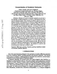
3.7 Generalized ensembles Let’s consider a system with x = {x1 , x2 , · · · } a vector of mechanical extensive variables and f the corresponding conjugate vector. Now imagine an equilibrated system in which both E and x can fluctuate. This system can be considered as a part of an isolated composite system in which the other part can be viewed as a big reservoir for both E and x (see also Fig. 3.1). Both, the energy En and xn fluctuate because the system is in contact with the bath, but E = Eb + En and x = xb + xn are constant. If the system is in one definite state n, then the number of states accessible from system plus

3.7 Generalized ensembles

111

the bath is: Ω(Eb , xb ) = Ω(E − En )Ω(x − xn ) , where we have assumed that fluctuations of the energy and extensive parameter x are independent.

Fig. 3.1 Illustration of a system immersed in a bath.

The probability of observing the system in a state n is given by Pn ∝ Ω(E − En , x − xn )

= Ω(E − En )Ω(x − xn )

= exp (ln (Ω(E − En )Ω(x − xn )))

= exp (ln (Ω(E − En ))) exp (ln (Ω(x − xn )))

Now we can express ln (Ω(E − En )) and ln (Ω(x − xn )) according to Taylor series for En � E and xn � x: d ln Ω + · · · ≈ ln Ω(E) − βEn , dE d ln Ω + · · · ≈ ln Ω(x) − f · xn , ln (Ω(x − xn )) = ln Ω(x) − xn · dx

ln (Ω(E − En )) = ln Ω(E) − En

(3.25) (3.26)

where �

� ∂ ln Ω , ∂E � �x ∂ ln Ω fi = . ∂xi E,xj�=i β=

(3.27) (3.28)

Finally we can write: Pn ∝ exp (−βEn − f · xn ) ,

(3.29)


where the proportionality constant is independent on the particular state of the system and it is determined from the normalization condition: � Pn = 1 . n

Hence,

Pn = Ξ −1 exp (−βEn − f · xn ) ,

where Ξ=

� n

exp (−βEn − f · xn ) ,

(3.30) (3.31)

are the probability distribution and partition function of the generalized ensemble. Thermodynamic values of E and xi are given through ensemble averages: � � � ∂ ln Ξ �E� = Pn E n = − , (3.32) ∂β f ,x n � � � ∂ ln Ξ �xi � = Pn xi,n = − (3.33) ∂fi T,E,xj�=i n

3.8 Isothermal-isobaric ensemble An example of the generalized canonical ensemble is the so-called isothermalisobaric ensemble or Gibbs ensemble. In the isothermal-isobaric ensemble, the temperature T , number of particles N and pressure p are held constant, but both, the energy E and volume V are allowed fluctuating. The conjugated fields that control these fluctuations are T (or β) and βp, respectively. We denote with n the state of system at volume Vn and energy En , then from Eq. (3.30) and Eq. (3.31) we get Pn = Ξ −1 exp (−βEn − βpVn ) , where Ξ=

� n

exp (−βEn − βpVn ) .

Using the Gibbs formula for the entropy � S = −kB Pn ln Pn n

(3.34) (3.35)

3.9 Grand canonical ensemble

= −kB

113

� n

Pn [− ln Ξ − βEn − βpVn ]

= −kB [− ln Ξ − β�E� − βp�V �] . This expression can also be written as: −kB T ln Ξ = �E� − T S − p�V � ,

(3.36)

which can be compared with the formula for Gibbs free energy: G = E − T S − pV . From this comparison we obtain G = −kB T ln Ξ = G(N, p, T )

(3.37)

Thus, it can be seen that Gibbs free energy G is a natural function of macroscopic variables of system N , p, and T .

3.9 Grand canonical ensemble Another very important application of generalized ensemble is grand canonical ensemble. This ensemble includes the set of all states of an open system at constant volume V . Both, the energy and number of particles are allowed fluctuating, and the conjugated fields that control the magnitude of these fluctuations are β and −βµ, respectively. Thus, if we denote with n the state with Nn particles and energy En , from Eq. (3.30) and Eq. (3.31), we get Pn = Ξ −1 exp (−βEn + βµNn ) ,

(3.38)

where Ξ is the grand canonical partition function given by � Ξ= exp (−βEn + βµNn ) .

(3.39)

Using the Gibbs formula for the entropy, we get � S = −kB Pn ln Pn

(3.40)

n

n

= −kB

� n

Pn [− ln Ξ − βEn + βµNn ]

= kB ln Ξ +

1 1 �E� − �N � . T T

Comparing this expression with the one for internal energy: E = T S − pV + µN , we obtain


pV = −kB T ln Ξ ,

(3.41)

which gives the free energy for the open system. Since the energy, E, depends on the volume, we can say that free energy pV for the open system depends on T , V and µ, which are also the nature macroscopic variables for grand canonical ensemble.

3.10 Grand isothermal-isobaric ensemble Grand isothermal-isobaric ensemble is defined as an ensemble with the fixed external pressure p, temperature T , and the chemical potential µ. Thus, in this ensemble, the energy E, volume V and number of particles N are allowed fluctuating. The conjugated fields that control these fluctuations are β, βp and −βµ, respectively. Therefore, the probability of observing the system in state n with volume Vn , energy En and number of particles Nn is found from Eq. (3.30) and Eq. (3.31) as: Pn = Ξ −1 exp (−βEn − βpVn + βµNn ) ,

(3.42)

where Ξ is the grand canonical partition function given by � Ξ= exp (−βEn − βpVn + βµNn ) .

(3.43)

Using the Gibbs formula for the entropy, we have � S = −kB Pn ln Pn

(3.44)

n

n

= −kB

� n

Pn [− ln Ξ − βEn − βpVn + βµNn ]

= kB ln Ξ +

1 1 1 �E� + p�V � − µ�N � , T T T

or T S = kB T ln Ξ + �E� + p�V � − µ�N � . This expression indicates that kB T ln Ξ = 0 , or Ξ=1, since T > 0.

3.11 Fluctuations

115

3.11 Fluctuations 3.11.1 Canonical ensemble We showed that each microstate n in canonical ensemble has a certain probability Pn given by expression Eq. (3.11). Since the number of different microstates is very large, we are not only interested on the probability of microstates (Pn ), but also on the probability of macrostate variables. For instance, the internal energy U . We first calculate the average internal energy �E� (or U ): � U ≡ �E� = E n Pn (3.45) n

1 � En e−βEn = Q n � � ∂ ln Q =− . ∂β N,V

Similarly, the second moment of U is � �E 2 � = En2 Pn

(3.46)

n

=

1 � 2 −βEn E e Q n n

1 � ∂ 2 −βEn e Q n ∂β 2 � � 1 ∂2Q = . Q ∂β 2 N,V =

Then, the variance of energy fluctuations can be obtained as: 2

2

�(δE) � = �(E − �E�) �

(3.47)

= �E 2 � − �E�2 �2 �� 1 ∂2Q ∂ ln Q = − Q ∂β 2 N,V ∂β N,V � � ∂�E� =− ∂β N,V

Since (∂�E�/∂T )N,V = CV is the specific heat, then we can further write

116 3 Hiqmet Kamberaj, International Balkan University, Email: [email protected] 2

�(δE) � = kB T 2 CV

(3.48)

Practically, this is a very important result, because it relates the amount 2 of spontaneous fluctuations, �(δE) �, with the degree of energy change with temperature, CV . Since the specific heat and the energy are extensive quantities, then they are of order N (the number of particles in the system). Thus, the ratio of the standard deviation of energy fluctuation to its average value is of order N −1/2 , i.e: � √ � � 2 �(E − �E�) � 1 kB T 2 C V = ∼O √ . �E� �E� N For large systems, such as N ∼ 1023 , N −1/2 becomes a very small number and we can consider the average value of energy as an accurate prediction of the experimental internal energy. For example, consider an ideal gas of structureless particles, we know that CV = and �E� =

3 N kB 2 3 N kB T 2

If we consider N ∼ 1022 , then the above ration is numerically ∼ 10−11 , which is a very small number.

3.11.2 Generalized ensemble For general statistical ensemble, from statistical mechanics we have � � ∂�x� 2 . �(δx) � = − ∂f T,E

(3.49)

The left hand side is always positive, and the right hand side determines the curve or convexity of the thermodynamical free energy.

3.11 Fluctuations

117

3.11.3 Isothermal-isobaric ensemble For isothermal-isobaric ensemble, x ≡ V and f ≡ βp, thus � � ∂�V � 2 �(δV ) � = − ∂ (βp) T,E � � ∂�V � ≥0. = −kB T ∂p T,E

(3.50)

The last inequality is true since from the condition of equilibrium stability discussed in the previous chapter, we got � � ∂�V � ≤0. ∂p T,E For this ensemble, the fluctuations of energy are given as; � � ∂�E� 2 �(δE) � = − , ∂β N,p which can further be written as � � ∂�H� − p�V � 2 �(δE) � = − ∂β N,p � � � � ∂�H� ∂�V � =− +p , ∂β N,p ∂β N,p

(3.51)

(3.52)

where �H� is the average value of the enthalpy: �H� = �E� + p�V � Using the relation of the specific heat at constant pressure: � � ∂�H� Cp = ∂T N,p we can write 2

�(δE) � = kB T

2

�

Cp − p

�

∂�V � ∂T

�

N,p

�

This expression can be simplified using the relation: � � � � ∂V ∂p C p = CV + T . ∂T N,V ∂T N,p

.

(3.53)


Substituting this expression in Eq. (3.53), we get � � �� ∂p ∂�V � 2 2 2 −p . �(δE) � = kB T CV + kB T T ∂T N,V ∂T N,p

(3.54)

Substituting the expression � � � � � � ∂�V � ∂V ∂p =− ∂T N,p ∂T N,V ∂p N,T into Eq. (3.54), we obtain 2

�(δE) � = kB T 2 CV � � �� ∂p ∂V ∂p 2 − kB T T −p ∂T N,V ∂T N,V ∂p N,T � � �2 � � � ∂p ∂V 2 −p . = kB T C V − k B T T ∂T N,V ∂p N,T

(3.55)

By direct comparison of expression given by Eq. (3.48) and the one given by Eq. (3.55), it can be seen that the energy fluctuations in canonical ensemble (with N , V and T constant) differ from the fluctuations in isothermal-isobaric ensemble (with N , p and T constant), namely by the term � � �2 � � � ∂V ∂p −kB T T −p ∂T N,V ∂p N,T which includes the change of pressure with temperature (at constant N and V ) and change of volume with pressure (at constant N and T ).

3.11.4 Grand canonical ensemble Formulas of the fluctuations for the grand canonical ensemble can be defined similarly to canonical ensemble. For instance, the fluctuations of the number of particles is given by: 2

2

�(δN ) � = �(N − �N �) � = �N 2 � − �N �2 . It can easily be shown that

3.11 Fluctuations

119

�N � = 2

�N � =

�

�

∂ ln Ξ ∂ (βµ)

�

,

(3.56)

T,V,µ

1 ∂2Ξ Ξ ∂ (βµ)2

�

.

(3.57)

T,V,µ 2

Substituting these two equations in the expression for �(δN ) �, we finally get � � ∂�N � 2 . (3.58) �(δN ) � = ∂ (βµ) T,V,µ 2

Note that �(δN ) � ≥ 0, hence, �

∂�N � ∂µ

�

T,V,µ

≥0.

Since �N � = nN0 , where n is the number of moles and N0 is the Avogadros number, we get � � ∂n ≥0, ∂µ T,V,µ which is one of the thermodynamic conditions of stability of system, obtained in the previous chapter, derived here in the context of statistical thermodynamics. Fluctuations of the energy are defined as: � � ∂�E� 2 �(δE) � = − . ∂β V,µ

(3.59)

The above relation is similar to the relationship found for the canonical ensemble, but it is different because the derivative is evaluated at constant N for the canonical ensemble and at constant chemical potential µ for the grand canonical ensemble. Hence, the energy fluctuations are different in the canonical and grand canonical ensembles. The reason for this difference between the fluctuations in grand canonical and canonical ensembles is not easy to determine from the above expression since the chemical potential is difficult to measure. The difference can be made explicit by using thermodynamics, in which case we identify the average energy E in the grand canonical ensemble with U . That is, since on holding V fixed �N � = �N (T, µ)� , (3.60) one has U = U (T, �N (T, µ)�) .

(3.61)


Thus, the differential of U can be written as � � � � ∂U ∂U dU = dT + d�N � (3.62) ∂T �N � ∂�N � T � � � �� ∂�N � ∂U ∂�N � ∂U dT + dT + dµ . = ∂T �N � ∂�N � T ∂T µ ∂µ T Hence, the derivative of U with respect to T with µ held fixed is given by � � � � � � � � ∂U ∂�N � ∂U ∂U = + (3.63) ∂T µ,V ∂T �N � ∂�N � T ∂T µ � � � � ∂�N � ∂U . = CN,V + ∂�N � T ∂T µ Therefore, the fluctuations of energy are given by � � � � ∂U ∂�N � 2 2 2 �(δE) � = kB T CN,V + kB T . ∂�N � T ∂T µ

(3.64)

As one can see, the first term of the energy fluctuation in the grand canonical ensemble is the same as energy fluctuations in the canonical ensemble where the number of particles and the volume are fixed and the other contribution (see second term in Eq. (3.64)) originates from the temperature dependence on the number of particles. We can further simplify the above expression to obtain more insight into the origin of the energy fluctuations in grand canonical ensemble. First, we can consider the differential of the internal energy U for one component system dU = T dS − pdV + µd�N � . (3.65) Dividing both sides by d�N � keeping T and V constant gives � � � � ∂S ∂U =T +µ. ∂�N � T,V ∂�N � T,V

(3.66)

Substituting the Maxwell equation � � � � ∂µ ∂S =− ∂�N � T,V ∂T �N �,V into Eq. (3.66) we obtain the first thermodynamic relation � � � � ∂µ ∂U = −T +µ. ∂�N � T,V ∂T �N �,V

(3.67)

3.11 Fluctuations

121

Dividing both sides of Eq. (3.62) by dµ keeping T and V constant, we obtain � � � � � � � � ∂�N � ∂U ∂�N � ∂U = =T , ∂µ T,V ∂�N � T,V ∂µ T,V ∂T µ,V Hence, �

∂�N � ∂T

�

= µ,V

1 T

1 = T

� �

∂U ∂�N � ∂�N � ∂µ

�

�

T,V

T,V

� �

∂�N � ∂µ

µ−T

�

(3.68) T,V

�

∂µ ∂T

�

�N �,V

�

.

(3.69)