Figure 1, a CDG specifies inter-component dependencies ... For example, the component A in the example CDG ...... Supercomputing '90, pages 2â11, Nov.
Prioritizing Component Compatibility Tests via User Preferences Il-Chul Yoon, Alan Sussman, Atif Memon, Adam Porter Department of Computer Science, University of Maryland, College Park, MD, 20742 USA {iyoon,als,atif,aporter}@cs.umd.edu
Abstract Many software systems rely on third-party components during their build process. Because the components are constantly evolving, quality assurance demands that developers perform compatibility testing to ensure that their software systems build correctly over all deployable combinations of component versions, also called configurations. However, large software systems can have many configurations, and compatibility testing is often time and resource constrained. We present a prioritization mechanism that enhances compatibility testing by examining the “most important” configurations first, while distributing the work over a cluster of computers. We evaluate our new approach on two large scientific middleware systems and examine tradeoffs between the new prioritization approach and a previously developed lowest-cost-configuration-first approach.
1 Introduction As today’s software systems become increasingly large and complex, they are subject to several trends. Increased reliance on third-party components: In practice, little software is developed entirely from scratch any more. Instead, majority of software is assembled from (third-party) components (e.g., libraries, tools, objects). While this practice allows complex systems to be developed quickly, it also creates problems for quality assurance. One such problem involves build testing. Because end-users often have different versions of third-party components installed on their computer systems (e.g., /usr/local/lib/gcc, Python, numerical libraries, etc.), software developers must ensure that their systems build correctly over all deployable configurations (combinations of components). We call this process of build testing multiple configurations compatibility testing. Because of the very large number of possible configurations comprising a complex software system, in practice, compatibility testing is a resource intensive process. Need for quick quality assurance: The practice of fre-
quent build testing has become extremely popular. Automated tools are deployed to build the latest version of the application on each check-in, periodically or overnight. Results from the process are expected to be quickly available to developers. Availability of clusters of machines and virtualization environments: As hardware costs decrease, quality assurance teams have access to powerful clusters of machines. Moreover, there is an increased use of virtualization environments, such as VMware Server, that allow developers to “mimic” different runtime environments. While this is desirable because different configurations can be built on different machines in parallel, it also creates the need for sophisticated test scheduling and management policies. Recognizing the above trends, in prior work we have developed Rachet, a process and infrastructure to support compatibility testing [13, 14]. The key features of Rachet are its ability to intelligently sample from a vast set of configurations, thereby reducing overall work, and to distribute the build process over multiple machines, including virtual machines. These features help to reduce overall turnaround time needed to perform compatibility testing. One major limitation is that Rachet always builds the lowest cost configuration first, completely ignoring developer preferences. For example, a developer may be more interested in configurations that (1) are composed of the latest versions of all components, or that (2) use a particular version of a specific component. It is impractical for developers to manually specify an ordering on the configurations to be tested. Rachet needs to be able to handle such preferences in an automatic and systematic way. In this paper, we present a prioritization mechanism that enhances Rachet by testing the configurations “most important” to developers first. We describe a mechanism by which developers can easily specify a preference order for configurations. We evaluate our new approach on two large scientific middleware systems. Our results explore the tradeoffs between the new prioritization approach and our previous “lowest cost configuration first” approach. In the next section, we give an overview of Rachet. Section 3 describes the user-preference based algorithms and
G1 {}
A F1 {G1}
*
E2 {G1} D2 {F1}
+ B
E1 {G1} D1 {F1}
E4 {G1}
E3 {G1}
B2 {E4}
D3 {F1}
B3 {E4}
B1 {E4}
F5
F4
F3
F2
C1 {E4}
E3
E4
E2
E1
E3
E2
E1
E3
E2
E1
E3
D3
D1
D2
D2
D1
D3
D2
D1
D3
D2
D1
D3
D Version Annotations
C *
*
E
F
Component A B C D E F G
* G
Versions A1 B1, B2, B3 C1, C2 D1, D2, D3 E1, E2, E3, E4 F1, F2, F3, F4, F5 G1
Constraints (ver(C) == C2) ĺ (ver(E) E3)
Figure 1. An Example System Model overall approach. In Section 4, we present results from empirical studies on two large software systems. Section 5 describes related work and Section 6 concludes with a brief discussion of future research plans.
2 Rachet Overview The Rachet process consists of four steps. First, developers model the system under test (SUT) using a formal representation consisting of two parts: (1) a directed acyclic graph called the Component Dependency Graph (CDG) and a set of (2) Annotations. As illustrated in the example in Figure 1, a CDG specifies inter-component dependencies by connecting components with AND and XOR relationships. For example, the component A in the example CDG depends on the component D and either one of B or C (captured via an XOR node represented by +). Annotations include version identifiers for components, and constraints between components and/or over configurations, written in first-order logic. Together, the CDG and annotations define the set of all valid configurations for the SUT. Second, developers determine which parts of the configuration space will be tested. Since it is normally infeasible to test the entire configuration space, Rachet employs a mechanism to systematically sample the space. One such sampling strategy is based on the observation that the ability to successfully build a component c is strongly influenced by the components on which c directly depends. In CDG terms, a component c directly depends on a set of components, DD, such that for every component, DDi ∈ DD, there exists at least one path, not containing any other component node, from the node encoding c to the node encoding DDi . From this definition, Rachet obtains relationships, called DD-instances, between versions of each component and versions of all other components on which it directly depends. A DD-instance is encoded as a tuple t = (cv , d) where cv is a version v of a component c; d is the dependency information used to build cv ; it is a set of versions of components on which c directly depends. The end result
B1 {E2}
B1 {E1}
A1 {B1 D2}
A1 {B1 D1}
B1 {E3} A1 {B1 D3}
C2
C2
C2
C1
C1
C1
B3
B3
B3
B2
B2
B2
A1
A1
A1
A1
A1
A1
A1
A1
A1
A1
A1
A1
Figure 2. An Example DD-coverage Test Plan of this strategy is a set of configurations to test. For this example, that set would include configurations in which all DD-instances for all system components are covered. We call this criterion DD-coverage. Third, Rachet automatically produces a set of configurations satisfying the test coverage criteria. To satisfy the DDcoverage criterion, for example, Rachet produces configurations where each DD-instance is covered by at least one configuration. For each DD-instance not yet covered, for every component in a CDG, Rachet adds appropriate DDinstances for components on which the component directly depends to the configuration under construction. (If multiple DD-instances are appropriate, we prefer one that is not covered yet.) This process is applied recursively until the configuration contains all DD-instances required to build the component version encoded by the initial DD-instance. Rachet uses Prolog as an external constraint checker to determine whether a configuration under construction violates any constraint (from the Annotations) during the recursive process. Fourth, Rachet combines the produced configurations into a tree data structure called a prefix tree. The prefix tree acts as a test plan in which each node corresponds to a DDinstance contained in the configurations; each path from the root node to a leaf node corresponds to a produced configuration. The rationale behind combining configurations is that we may reduce the overall time to execute configurations by reusing configurations partially completed (built) by a machine. A test plan with DD-coverage for the example model is shown in Figure 2. Note that each node in the tree represents a DD-instance – it is of the form (cv , d) where cv is a component version and d is a set of versions of components on which cv directly depends. Finally, Rachet executes the test plan by scheduling configurations to multiple machines and collecting results. Instead of distributing full configurations, Rachet distributes partial configurations, called tasks, to increase the reuse of partial builds that share sub-configurations (prefixes in the tree) across configurations. We have examined three plan execution strategies to determine the task to distribute next for a client request: (1) a parallel depth-first strategy that tries to maximize the reuse of tasks locally available in each client, (2) a parallel breadth-first strategy that tries to maximize task parallelism throughout plan execution, and (3) a hybrid strategy that combines the benefits of
Global Coordinator
Local Coordinator
CDG + Ann
Task Manager
Configuration Generator Test Plan Builder
Task Manager VMware Task Manager VMware VMware
Plan Execution Manager
ReqQ
LC handler
ResQ
LC handler
LC handler
VM Coordinator VM Coordinator VM CoordinatorVM Cache VM Cache
Test DB
VM Cache
Figure 3. Rachet Architecture Overview the depth-first and breadth-first strategies. The hybrid strategy achieves maximum parallelism in its initial execution stage by scheduling the test plan in breadth-first order, and then tries to increase task reuse locality by scheduling tasks in depth-first order. Figure 3 gives an overview of the architecture of Rachet. The global coordinator is responsible for taking the CDG and annotations as input, producing the set of valid configurations, and creating the test plan. A plan execution manager distributes the build tasks to various local coordinators residing in different physical machines, also called client machines. The actual component builds are done in a virtual machine (VM). When a task is successfully completed, i.e., all component versions contained in the task are built successfully without errors, the VM state realizing the task is cached in the client machine for later reuse. The global coordinator is made aware of all successful and failed builds so that it can adapt the plan execution accordingly. One example of plan adaptation is Rachet’s use of contingency planning when a component build fails. A build failure for a component version encoded by a DDinstance prevents building DD-instances encoded by nodes in subtrees rooted at all nodes encoding the identical DDinstance.1 In this case, Rachet’s global coordinator dynamically modifies the test plan by removing sub-trees and creating new configurations to build the DD-instances encoded by the removed nodes in alternate ways, if possible.
3 A Preference-Driven Plan Execution Software developers are often more interested in some configurations than others. For instance, they may be more interested in configurations with recently changed components or in those that use more popular versions of particular components. In this section, we present a methodology for executing test plans in a way that reflects differing developer priorities. We first describe how developers specify 1 Multiple nodes may encode an identical DD-instance when it is added to multiple configurations in the process of producing configurations.
their preferences. We then discuss how we use these preferences to determine the order in which configurations are tested. Our key objectives are to conduct testing efficiently while producing test results for higher preference configurations before ones with lower preference.
3.1
Specifying Preferences
Modern systems can have an enormous number of configurations. Thus, it is impractical for developers to explicitly specify preferences for all configurations to be tested. Therefore we use a simple method in which developers first express preferences between all system components. Then for each component they express preferences between all versions of that component. User preferences may be represented in any form that specifies relative user interest across component versions. For this work, we encode version preferences as positive integer values with larger values indicating higher preference. If developers do not care to specify certain preferences, Rachet assigns a default preference – lower than all developer-specified preferences – in which components closer to the top node of the CDG are preferred over lower ones, and more recent versions of a component are preferred over older ones. We interpret these partial preference assignments as capturing the developers’ preferred ordering of test results. That is, we believe they want test results for configurations with high-preference versions of high-preference components before test results of other configurations.
3.2
Using Developer Preferences
In this section we give more detail on how we use developer preferences to guide the test process. Given a set of developer preferences we could just opportunistically test configurations containing the most preferred components and component versions first. This would, however, be quite inefficient. As our previous work clearly shows, intelligently coordinating build effort across multiple configurations can save substantial time and effort. Therefore, our testing approach needs to consider not only developer preferences, but also the structure of the test plan so that total test effort can be reduced. To this end we transform developer preferences (expressed over components and component versions) into preferences over nodes in the test plan. Remember that every node in the test plan represents the building of a partial system configuration. That is, a test plan node represents building all components represented by the nodes on the path from the root node in the plan to that node. When building a node from scratch, the start of the path will be the root node of test plan, while building from a cached test
Pref. Pref. Pref. Pref. Pref.
1 2 3 4 5
A A1
Component & Version B C D E F B1 C1 D1 E1 F1 B2 C2 D2 E2 F2 B3 D3 E3 F3 E4 F4 F5
3.3 G G1
Table 1. Example Preference Assignments result means the start of the path is somewhere in the middle of the path. Logically, component version preferences are represented as vectors, called preference vectors. A preference vector has one element for each component, with these elements ordered by component preference.2 The elements values are assigned as follows: for a component C with version cv , each element takes the value 0, except for the element associated with C, whose values takes the preference assignment of cv . For example, consider the system shown in Figure 1. Assume that the components A–G have preferences 7–1 respectively. Assume further that the version preferences for each component are sequentially numbered preferences starting at 1. This data is represented graphically in Table 1. Given these preference assignments, we write the preference vector for component B, version B3 , for example, as (0, 3, 0, 0, 0, 0, 0). This because B is the second highest preferred component and because version B3 has preference assignment 3. Similarly, the preference vector for component F , version F3 is (0, 0, 0, 0, 0, 3, 0) Given the component preference vectors we can now define preference vectors for every possible step in the test process. For a given path we do this by taking a component-wise vector sum of each node in the path. For example, going back to Figure 2, consider the gray-shaded leaf node with the label starting with A1 . To build that node from scratch, we must build each node from the root of the test plan to this node. Therefore, we compute the preference vector for this entire task by summing the preference vectors of all nodes appearing in that path: G1 : (0, 0, 0, 0, 0, 0, 1), F1 : (0, 0, 0, 0, 0, 1, 0), E2 : (0, 0, 0, 0, 2, 0, 0), D2 : (0, 0, 0, 2, 0, 0, 0), B1 : (0, 1, 0, 0, 0, 0, 0), A1 : (1, 0, 0, 0, 0, 0, 0). This gives a resulting preference vector of (1, 1, 0, 2, 2, 1, 1). Note that the third vector element is zero because component C is not contained in the task. In the next section we describe how we use path preferences to guide execution of the test plan. 2 To simplify the presentation we restrict discussion to cases in which preference assignments are unique. Rachet can, however, handle nonunique component preferences by allowing an element in a preference vector to encode version preferences for multiple components with identical preferences.
Preference-guided Plan Execution
As mentioned earlier, Rachet clients (local coordinators) repeatedly request tasks from the Rachet global coordinator. For each request, the global coordinator selects the task to execute next in a greedy fashion, by first ordering the task preferences associated with all nodes not yet assigned to any client. Logically, this ordering is done by lexicographically sorting task preference vectors. We give a high-level description of the selection process in Algorithm 1. Algorithm 1 Schedule a task to execute, considering both user preference and task execution cost Algorithm Prioritized-Execution(Plan, C, W) 1: // C: requesting client, W : window size 2: TaskSet ← ∅ 3: for each task t for not-yet assigned node n ∈ P lan do 4: lt ← # of comps to build for t reusing a local task 5: rt ← # of comps to build for t reusing a remote task 6: stealt ← # of clients containing a cached task for t 7: TaskSet ← TaskSet ∪ < t, preft , lt , rt , stealt > 8: end for 9: Sort TaskSet by pref 10: return a task with minimum lt , or a task with minimum stealt among the first W tasks in TaskSet. (rt is used to break tie with identical stealt ) In the algorithm, we first extend each candidate task t with auxiliary information. lt is the number of component versions that must be built to execute t reusing the best locally available cached task in which a subset of the component versions contained in t are already built. When multiple clients are used to execute a test plan, this information may be used to maximize task reuse in each client, taking advantage of previous tasks executed by a client. The variables rt and stealt are used to reduce redundant work across clients. rt is the number of component versions that must be built for task t, reusing the best task cached in a client. stealt is the number of clients that have at least one cached task that may be reused to execute t. When there is no task that can reuse a locally available task, Rachet executes a task that minimizes stealt . rt is used to break ties when there are multiple candidate tasks with an identical stealt value. Note that Algorithm 1 has to be repeatedly invoked for each task request, since the plan execution state (including cache states at clients) changes continuously and the auxiliary information used in scheduling tasks depends on which client requests a new task. Although the auxiliary information may be used to decrease overall plan execution time by efficiently sharing the effort needed to execute the tasks for different configurations, the most important concern for developers is still the
task preferences. Therefore, we sort the TaskSet in task preference order. We always execute the first task in the set to produce more highly preferred results earlier.3 However, due to the large size of cached tasks and limited cache space in each client, scheduling tasks by only taking into account preference order may increase the number of remote task cache hits and as a result, the rate of local cache reuse drops and total plan execution time can increase compared to a solely cost-based scheduling policy. Rachet allows developers to determine how rigidly they want their preferences enforced. With a strong preference, the test plan always selects the most highly preferred configuration that has not yet been assigned to a client to be executed (or has already completed), and with a weaker preference the scheduling considers other factors, such as task reuse locality, that help to minimize the overall plan execution time, in exchange for allowing less highly preferred configurations to be executed earlier. Developer preference strength is expressed via a window size parameter, denoted W. As shown in Algorithm 1, we inspect the first W tasks in the TaskSet and select the task that requires building the fewest components, considering reuse of locally cached task results for that client. This means that less highly preferred tasks can be selected if they can be executed at low cost by reusing the results from previously executed tasks at that client. If no locally cached task result can be used, the scheduling algorithm selects a task for execution that has the smallest overlap with tasks currently being executed by other clients, to maximize the potential for future task result reuse. An interesting case occurs when the window size is set to a value greater than or equal to the number of nodes in the test plan. In that case, since we first try to execute tasks that reuse locally cached task results, and then try to reuse a remotely cached task result, the test plan is executed in a similar order to the hybrid plan execution strategy described in Section 2, that minimized overall plan execution time as shown in our prior work.
4 Evaluation We now evaluate our prioritization approach by constructing two scenarios that often occur during compatibility testing. In the first scenario, we want to test full configurations that are based on more recent versions of the SUT. In the second scenario, we prefer configurations that use recent versions of specific components required to build the SUT. In this section we describe these scenarios, describe two large software systems to which our prioritization technique is applied, and present benefits and tradeoffs of the overall approach. We specifically want to compare 3 However, results may still not be produced in preference order because of varying component, and therefore configuration, build times.
our prioritization approach with our last-best-known hybrid approach measuring the time it takes to test preferred configurations. We also want to study the tradeoffs involved in varying the window size parameter of Algorithm 1, and in varying the number of clients used to execute the test plan.
4.1
Subject Systems
We use two large software systems for our experiments, namely InterComm and PETSc. InterComm4 is a middleware library that supports coupled scientific simulations by redistributing data in parallel between data structures managed by multiple parallel programs. To provide this functionality, InterComm relies on several system components, including multiple C, C++ and Fortran compilers, parallel data communication libraries, a process management library and a structured data management library. Each component has multiple versions and there are dependencies and constraints between the components and their versions. PETSc (Portable, Extensible Toolkit for Scientific computation)5 [2] is a collection of data structures and interfaces used to develop scalable high-end scientific applications. Similar to InterComm, PETSc is designed to work on many Unix-like operating systems and depends on multiple compilers and parallel data communication libraries to provide interfaces and implementations for serial and parallel applications. To enhance the performance of applications developed using PETSc, it also relies on third-party numerical libraries such as BLAS [7] and LAPACK [1], and uses Python as a deployment driver. We have used these systems in previously reported work [13, 14], and for this study we have extended models for the systems by adding more versions of some components and also by specifying preferences on components and their versions.
4.2
Modeling the Subjects
Modeling the subject systems involved creating the CDG and annotations for each system. This process is currently manual and took almost a week. Dependencies between components for the systems are shown in Figure 4. We show a combined CDG, since InterComm and PETSc share many components. Table 2 shows the version annotations for the components in the CDG. Component versions added for this paper are shown in bold font in the table. In addition to the CDG and version annotations, we enforced several constraints on the configurations for the systems. First, if multiple GNU compilers are used (gcr, gxx, gf and gf77) in a configuration, they must have the same version identifier. Second, only a single MPI component 4 http://www.cs.umd.edu/projects/hpsl/chaos/ResearchAreas/ic 5 http://www.mcs.anl.gov/petsc/petsc-as
petsc
ic
*
*
python
ap
lapack
pvm
* +
*
*
mch
lam
*
*
* + gf
pf
gf77
* gxx
Version 1.1, 1.5, 1.6 2.2.0 2.3.6, 2.5.1 1.0 2.0, 3.1.1 0.7.9 3.2.6, 3.3.11, 3.4.5 6.5.9, 7.0.6, 7.1.3
mch gf gf77 pf gxx pxx mpfr
1.2.7 4.0.3, 4.1.1 3.3.6, 3.4.6 6.2 3.3.6, 3.4.6, 4.0.3, 4.1.1 6.2 2.2.0, 2.3.2
gmp
4.2.1, 4.2.4
pc gcr
6.2 3.3.6, 3.4.6, 4.0.3, 4.1.1 4.0
blas
+
pxx
Comp. ic petsc python blas lapack ap pvm lam
mpfr * * gmp
fc
+
Description InterComm, the SUT PETSc, the SUT Dynamic OOP language Basic linear algebra subprograms A library for linear algebra operations High-level C++ array management library Parallel data communication component A library for MPI (Message Passing Interface) standard A library for MPI GNU Fortran 95 compiler GNU Fortran 77 compiler PGI Fortran compiler GNU C++ compiler PGI C++ compiler A C library for multiple-precision floating-point number computations A library for arbitrary precision arithmetic computation PGI C compiler GNU C compiler Fedora Core Linux operating system
Table 2. Component Version Annotations
pc * gcr * fc
Figure 4. Combined CDG for Subject Systems (i.e., lam or mch) can be used in a configuration. Third, only one C++ compiler, and only one of its versions (gxx version X or pxx version Y) can be used in a configuration. Fourth, if both a C and a C++ compiler are used in a configuration, they must be developed by the same vendor. (i.e., GNU Project or PGI). Based on the PETSc documentation, we applied an additional constraint for PETSc: compilers from the same vendor must be used to build the PETSc and MPI component. These constraints helped eliminate those configurations that we knew a priori would not build successfully.
4.3
Scenarios
As mentioned earlier, we constructed two scenarios to evaluate our approach. In the first scenario, developers want to test configurations that contain recent versions of the SUT. This scenario was actually encountered during the development of InterComm. When InterComm version 1.6 was released, the InterComm developers wanted to buildtest recent versions of InterComm. In addition, they also preferred to test configurations based on more recent versions of other components; they believed that a large portion of their user base had already updated the system components on their machines to recent versions. To meet this requirement, we assigned components pref-
erence ranks in the InterComm model by traversing the CDG in reverse topological order. For version preferences, higher values are assigned to recent component versions (the oldest version had value 1). We applied the same preference requirements for the PETSc model. In the second scenario, developers prefer to test configurations that contain recent versions of specific components required to build the SUT. Specifically, for the InterComm and PETSc model we model that developers prefer configurations containing recent version of the MPFR and the GNU MP component. Thus, we set high preference ranks for those components, and set higher version preference values for recent versions.
4.4
Test Planning and Execution
From the CDG and annotations, there are a total of 639 DD-instances for components in the InterComm CDG, and Rachet produced 476 configurations satisfying the DDcoverage criterion. These configurations altogether contain 4421 component versions to build, but the actual number of component versions to build is reduced to 1908 since the configurations are combined by Rachet into a single test plan. For PETSc, there are 185 DD-instances and Rachet produced 88 configurations that contain 846 component versions, which is reduced to 522 components in the test plan. We first ran actual builds to execute test plans for InterComm and PETSc and obtained compatibility results for DD-instances of components in the models. For the InterComm model, 134 out of 639 DD-instances were tested without errors, which means that there were 134 successful ways to build component versions (18 for the top-level In-
Config Completion Time (Hybrid,InterComm,Scenario 1) 80
Success Failure
70 60 Elapsed Time (hrs)
terComm component). A total of 58 DD-instances failed to build (3 for InterComm). The remaining 447 DD-instances were not tested because there was no successful way to build at least one of its required component versions. For example, all DD-instances to build the InterComm component version 1.5 with the PVM component version 3.2.6, which is a component on which the InterComm directly depends, could not be tested because all feasible ways to build the PVM component version failed. For the PETSc model, 107 out of 185 DD-instances were tested successfully (8 for the top-level PETSc component) and 62 DD-instances failed (56 for PETSc). The remaining 16 DD-instances were not tested.
50 40 30 20 10 0 0
200
400
600 800 1000 Configuration Preference
1200
1400
1600
Config Completion Time (Prioritized,InterComm,Scenario 1,W=1)
4.5
80
Simulations
Success Failure
70
Elapsed Time (hrs)
60 50 40 30 20 10 0 0
200
400
600 800 1000 Configuration Preference
1200
1400
1600
Config Completion Time (Hybrid,PETSc,Scenario 1) 30
Success Failure
25 Elapsed Time (hrs)
In the remainder of this study, we use the results of the actual test runs, including whether the tests were successful or failed and the execution times to build each component on top of the components on which it directly depends, to simulate different test plan execution strategies (prioritized vs. hybrid), using different number of clients (4, 8, 16, 32), and using different window sizes (1, 16, 256, 2048) - window size only matters for the prioritized strategy. In all, we simulated the 20 possible combinations across the dimensions (4 for the hybrid and 16 for the prioritized strategy). For each plan execution we recorded the time when configurations succeeded or failed. A configuration succeeded if all component versions in the configuration built without errors. We say a configuration failed if either its build script returned errors or one of the components on which it depends failed. Note that if a component version encoded by a DD-instance in a configuration failed, then all configurations that contain the DD-instance also fail. Thus, when a DD-instance appears in several branches in a test plan, multiple configurations fail simultaneously.
20 15 10 5 0 0
20
40
4.5.1 Prioritized vs. Hybrid
60 80 100 Configuration Preference
120
140
Config Completion Time (Prioritized,PETSc,Scenario 1,W=1) 30
Success Failure
25 Elapsed Time (hrs)
Figure 5 shows times at which configurations for the subject systems succeeded (shown as diamonds) or failed (shown as plus signs). The top two graphs are for InterComm and the bottom two are for PETSc, while the top graph for each system is for the hybrid plan execution strategy and the bottom graph is for the prioritized strategy. The x-axis in each graph shows all configurations, sorted by their preference order, i.e., the leftmost is the most preferred configuration. The y-axis shows the time taken to test the configuration. In this result, we use a window size of 1 and the number of client machines is 4. From these plots, we observe that the prioritized strategy achieved results for highly preferred configurations quickly compared to the hybrid strategy. The hybrid strategy achieved some results for highly preferred configurations almost at the end of the plan execution.
20 15 10 5 0 0
20
40
60 80 100 Configuration Preference
120
140
Figure 5. The prioritized strategy achieves results for highly preferred configurations earlier compared to the hybrid strategy.
Plan Execution Times with Variying Number of Machines 80 70
Plan Execution Times in Different Window Sizes 80
Prioritized, W=1 Hybrid
60
60 Elapsed Time (hrs)
Elapsed Time (hrs)
Prioritized, W=1 Prioritized, W=16 Prioritized, W=256 Prioritized, W=n Hybrid
70
50 40 30 20
50 40 30 20
10
10
0 M=4 M=8 M=16 M=32 M=4 M=8 M=16 M=32 --------- Scenario 1 ----------------- Scenario 2 --------Number of Clients Used for each scenario (InterComm, W=1)
0 Scenario 1
Scenario 2
Scenario with Various Window Sizes for InterComm
Figure 6. Time difference between the prioritized and the hybrid strategy decreases with more machines.
Figure 7. The prioritized strategy executes a test plan faster with larger window size, for 4 client machines.
Failed configurations form multiple bands in the graph for the prioritized strategy. This is because multiple configurations failed simultaneously when a component version failed to build, and because many of those configurations were different by only one or two DD-instances so had similar priorities. Each plot in Figure 5 contains different number of configurations for the prioritized and hybrid plan execution strategies because Rachet applies contingency planning when there are build failures, so produces additional configurations to build those DD-instances affected by the failures in alternate ways. The number of additional configurations differs depending on the time and the order failures are discovered. The graphs for InterComm contain almost ten times more configurations than graphs for PETSc because there were initially 476 configurations in the InterComm model compared to 88 for PETSc. Moreover, InterComm had many failures for components represented by intermediate component nodes in the CDG. We also observed that plan execution with the prioritized strategy overall took longer than for the hybrid strategy. The prioritized strategy took 48% and 19% more time for InterComm and PETSc, respectively, for a window size of 1. This is mostly attributed to low task reuse locality during plan execution. When we strongly guide the plan execution by user preference (window size 1), Rachet always schedules the most preferred task to a requesting client, without considering potential cost savings from reusing task results already cached in the client.
ure 6, the time difference between the prioritized and the hybrid strategy decreases for both scenarios for InterComm as the number of clients increases. We infer that the communication time spent for transferring task results (i.e., virtual machines) across clients is overlapped more with the time to build components in parallel when there are more clients, since more tasks are executed in parallel. 4.5.3 Varying Window Size Algorithm 1 enables developers to control preference guidance by modifying the window size. A window size of 1 means that developers only care about their preferences, not overall plan execution cost. In this situation, Rachet always schedules the most preferred configuration for any client task request. As the window size increases, Rachet considers other factors, including task reuse locality, that can reduce the overall plan execution time. Figure 7 shows that the InterComm test plan executed faster with larger window sizes for both scenarios. When the window size is equal to or greater than the number of nodes in a test plan (the case with W = n), the execution time with the prioritized strategy was comparable to the hybrid strategy. In this case the prioritized strategy ignores the developers preferences, and instead executes the test plan so as to maximize reuse of locally stored tasks and minimize redundant work across clients. The cost to gain the improved overall performance, as seen in Figure 8, is that test results for less highly preferred configurations are produced earlier than some more highly preferred configurations with larger window sizes.
4.5.2 Varying the Number of Clients The prioritized strategy took more time to execute a test plan. However, we observed an interesting result when we increased the number of clients for testing. As seen in Fig-
4.5.4 Quantitative Analysis In the previous sections, we have measured the costs and benefits of the prioritized strategy by visually inspecting
Config Completion Time (Prioritized,InterComm,Scenario 1,W=16) 80
Config Completion Time (Prioritized,InterComm,Scenario 1,W=256) 80
Success Failure
70
70
80
40 30
60 Elapsed Time (hrs)
50
50 40 30
50 40 30
20
20
20
10
10
10
0
0 0
200
400
600 800 1000 Configuration Preference
1200
1400
1600
Success Failure
70
60 Elapsed Time (hrs)
Elapsed Time (hrs)
60
Config Completion Time (Prioritized,InterComm,Scenario 1,W=n)
Success Failure
0 0
200
400
600 800 1000 Configuration Preference
1200
1400
1600
0
200
400
600 800 1000 Configuration Preference
1200
1400
1600
Figure 8. As window size increases, less highly preferred configurations may be executed earlier than more highly preferred ones.
If all configurations finish testing in preference order than this metric will always be 1. In fact, for many of our experiments using the prioritized strategy with a window size of 1, the metric stayed very close to 1. However, in some cases test results come out of order. This occurs for several reasons. First, the times to build component versions contained in various configurations are different, and client machine speeds also vary. Although we schedule more highly preferred configurations earlier, results for those configurations may be produced out of order. Second, when we fail to build a component version encoded by a DD-instance, multiple configurations that contain the DD-instance are marked to fail at the same time, while other more highly preferred configurations are still being executed. Figure 9 shows the conformance to preference order for successfully completed configurations, when we execute the InterComm test plan for the first scenario with the hybrid strategy and with the prioritized strategy, for different window sizes. We showed results after applying a smoothing technique called Loess smoothing [5, 6]. As seen in the figure, with a window size of 1 the plan execution conforms completely to developer preferences and that the degree of conformance drops as we increase the window size. An extreme case is when we execute the plan with a window size equal to the plan size. For that case, the prioritized strategy shows similar behavior to the hybrid strategy, since both strategies execute the test plan completely ignoring the developer specified preferences.
Conformance to Preference Order (InterComm, Scenario 1) 1
Prioritized (W=1) Prioritized (W=16) Prioritized (W=256)
0.8 Prioritized (W=n)
0.6 Ratio
patterns in the scatter plots in Figures 5 and 8. To evaluate the results more quantitatively, we developed a metric to measure conformance to preference order. Specifically, whenever a configuration finishes test, we compute the ratio between: 1) the number of already-tested configurations whose preference was greater than the current configuration’s preference and 2) the number of already-tested configurations.
Hybrid
0.4
0.2
0 0
0.1
0.2
0.3
0.4 0.5 0.6 Time Proportion
0.7
0.8
0.9
1
Figure 9. Conformance to preference order weakens as window size increases.
5 Related Work There have been several studies that incorporate user requirements into test case prioritization. Bryce et al. [4] describe a technique to prioritize test cases that cover pairwise interaction between factors when testers have different priorities between factors and their levels. They showed that test cases that take into account user priorities quickly achieved higher coverage for interactions in which users have more interest. Srikanth et al. [10, 11] used consumer priorities on requirements to prioritize system-level test cases. We share with those approaches the basic idea of considering user requirements to prioritize build tests. Continuous integration [3] recommends that developers integrate changes made every few hours into the complete software system and inspect whether those changes cause problems. Continuous integration also suggests testing whether those changes cause problems for configurations that mimic expected field configurations [8]. This approach has been highly advocated since it can be applied to many software projects with relatively low effort and also because problems originating from the difference between
development and field configurations can be detected early in the software development process [9]. Our approach is complementary to continuous integration. Rachet can be used to produce a set of field configurations and then test the configurations that developers think are most likely to appear in the field so that they are tested early in the test process. Such an approach would allow developers to perform integration testing on preferred configurations within the time allowed for each round of integration, in a seamless way without any developer intervention, and effectively utilize a set of available test resources. As an approach to support automated software compatibility testing, Rational, IBM and VMware have jointly developed a solution called Test lab automation [12]. Although this approach provides developers with an automated environment for testing software systems in multiple configurations without modifying the persistent state of test resources, the number of configurations can be very limited because developers are responsible for creating the configurations. In addition, developers must also directly determine the order in which the desired configurations are tested. Compared to this approach, Rachet automatically produces a set of configurations that effectively test intercomponent compatibility, and also enables executing tests in parallel. Our process does not require any intervention from developers after they model their software system and specify preferences.
6 Conclusion and Future Work In this paper we have presented a method for prioritizing the order in which configurations are executed, taking into account developer preferences. The goal is to obtain test results for configurations of higher importance early, in resource-constrained test environments. To accomplish this goal, we have developed methods that aid developers in specifying their preferences in a straightforward way, and also shown algorithms that intelligently schedule configurations considering specified preferences. Results from our empirical studies show that our techniques can help developers achieve results for preferred configurations early in the overall testing process, by guiding plan execution to consider the developer specified preferences. In the future, we will investigate how to apply the prioritization techniques when compatibility testing needs to be performed repeatedly. Considering properly the results from prior test plan executions can allow not re-executing a large portion of the test plan that has already been determined to work correctly. While the benefits of such a strategy are clear, the question is how to best integrate both test plan execution history information and update information to component versions that would invalidate prior test execution results, to best schedule a new round of testing.
Acknowledgments This research was supported by NSF grants #CCF0447864, #ATM-0120950 and #CNS-0615072, the Office of Naval Research grant #N00014-05-1-0421, and NASA grant #NNG06GE75G.
References [1] E. Anderson, Z. Bai, J. Dongarra, A. Greenbaum, A. McKenney, J. D. Croz, S. Hammarling, J. Demmel, C. H. Bischof, and D. C. Sorensen. LAPACK: A portable linear algebra library for high-performance computers. In Proc. of Supercomputing ’90, pages 2–11, Nov. 1990. [2] S. Balay, K. Buschelman, V. Eijkhout, W. D. Gropp, D. Kaushik, M. G. Knepley, L. C. McInnes, B. F. Smith, and H. Zhang. PETSc users manual. Technical Report ANL95/11 - Revision 2.3.2, Argonne National Lab., Sep. 2006. [3] K. Beck. Extreme Programming Explained: Embrace Change. Addison-Wesley, 1999. [4] R. C. Bryce and C. J. Colbourn. Test prioritization for pairwise interaction coverage. ACM Software Engineering Notes, 30(4):1–7, Jul. 2005. [5] W. Cleveland. Robust locally weighted regression and smoothing scatterplots. Journal of the American Statistical Association, 83:829—836, 1979. [6] W. Cleveland and S. Devlin. Locally weighted regression: An approach to regression analysis by local fitting. Journal of the American Statistical Association, 83:596–610, 1988. [7] J. Dongarra, J. D. Croz, S. Hammarling, and I. S. Duff. A set of level 3 basic linear algebra subprograms. ACM Transactions on Mathematical Software, 16(1):1–17, Mar. 1990. [8] M. Fowler. http://martinfowler.com/articles/continuousinte gration.html, May 2006. [9] B. Rumpe and A. Schr¨oder. Quantitative survey on Extreme Programming projects. In Proceedings of the 3rd Int. Conference on Extreme Programming and Flexible Processes in Software Engineering, pages 95–100, May 2002. [10] H. Srikanth and L. Williams. On the economics of requirements-based test case prioritization. ACM Software Engineering Notes, 30(4):1–3, Jul. 2005. [11] H. Srikanth, L. Williams, and J. Osborne. System test case prioritization of new and regression test cases. In Proceedings of 2005 Int. Symposium on Empirical Software Engineering, Nov. 2005. [12] VMware Inc. Streamlining software testing with IBM, Rational and VMware: Test lab automation solution, 2003. [13] I.-C. Yoon, A. Sussman, A. Memon, and A. Porter. Directdependency-based software compatibility testing. In Proc. of the 22st Int’l Conf. on Automated Software Engineering, Nov. 2007. [14] I.-C. Yoon, A. Sussman, A. Memon, and A. Porter. Effective and scalable software compatibility testing. In Proceedings of the 2008 Int. Symposium on Software Testing and Analysis (ISSTA 2008), pages 63–74, Jul. 2008.