Priority Cycle Time Behavior Modeling for ...

Priority Cycle Time Behavior Modeling for Semiconductor Fabs Shi-Chung Chang1,2

Bo-Jiun Liao1

[email protected] 1

Yu-Ting Kao1

Argon Chen1

[email protected] [email protected] [email protected] Graduate Institute of Industrial Engineering, National Taiwan University 2 Dept. of Electrical Engineering, National Taiwan University Taipei, Taiwan, R.O.C. 10617

Abstract—Semiconductor wafer fabrication factories (fabs) often offer wafer manufacturing services of multiple priorities in terms of differentiated cycle time-based targets and fab production must be planned accordingly. This paper aims to develop modeling methods and fab behavior models to capture cycle times of differentiated manufacturing services for semiconductor supply chain management. A novel, hybrid decomposition approximation-based priority queueing network model is designed to characterize how cycle times of individual priorities (PCTs) are affected by wafer release rates and fab capacity utilization. The approach integrates queueing network analyzer that approximates production flow behaviors among tool groups, sequential decomposition approximation among priorities, fixed point iteration to exploit the re-entrant flows and an empirical data-based model tuning technique. Model tuning and validation by comparison with simulation results demonstrate that the decomposition approximationbased models yield quick and good quality estimations of PCTs and related performance indices. The fab models thus constructed enable efficient what-if analysis for supply chain management of differentiated manufacturing services. Keywords- priority; cycle time; modeling; semiconductor fab; hybrid decomposition approximation, queueing network

I. INTRODUCTION A supply chain is a system of nodes that provides manufacturing services—in fact, a variety of services. Services differentiation, namely, prioritization, is common in operations of semiconductor supply chains (SSC, Figure 1). It affects how to allocate resources and charge prices. Such a new paradigm of manufacturing services requires new methods of operation control. Challenges are incurred by service prioritization - how to evaluate cycle-time based fab performance with priority with reasonable accuracy in short computation time, and how to achieve model scalability and predictability with respect to differentiation of services and variability that are exacerbated by the increasing product varieties and process variations in the chains. Priority service discipline is common in foundry fab operations and is critical to service differentiation. To provide service with differentiable ensures that the quality of service (QoS), allocation of manufacturing capacity and pricing of services have to be dependent of and differentiated by QoS requirements. Product, process and operation variability affects the performance of individual service nodes such as tool groups and fabs and chains/networks of service nodes. In order to predict the behavior of a SSC that provides differentiated services, research is needed in the following aspects: predictable and scalable performance

metrics with respect to the chain structure, and fundamental understanding of the behavior of service nodes and chains with respect to variability. Among the SSC service nodes, fab is the most expensive, complicated, and important. So this study is aimed at the behavior modeling of a fab and provides a cornerstone model for supply chain management. The model characterizes how cycle time of individual priorities (PCT) is affected by release rate and fab capacity utilization. The behavior model describes the relationship between output performance metrics and inputs, which are characterized by not only mean values but also variability. In this paper, we investigate the behavior modeling problem and develop fab behavior models and modeling methods that enhance the scalability and predictability of SSCs with respect to varieties, and differentiability of services. The input/output relationship of a fab is modeled as a network of priority service nodes. Such a priority network captures factors and effects of variations throughout the network model. The model is scalable and allows chain/network performance metrics to be decomposed into per node and per priority metrics. It has also predictability that allows very quick evaluation of mean and variability of both nodal and system output performance metrics such as cycle times under various priority input, resource allocation and sources of variations. The fab behavior model thus provides a cornerstone model to SSC management. The remainder of this paper is organized as follows. In Section II, a fab is modeled as a priority open queueing network (OQN). An innovative, hybrid decomposition approximation-based approach for such a priority OQN is then developed. Section III presents the validation results of the modeling method and a model tuning method. Section IV concludes the paper. II. FAB BEHAVIOR MODELING BY HYBRID DECOMPOSITION OF PRIORITY NETWORK Consider a fab with multiple part priorities, failure prone machines, and re-entrant process flows. We model the fab as a failure-free, batch-free, deterministic-feedback and priority open queueing network (OQN). Then we develop an innovative, hybrid decomposition approximation-based approach for such a priority OQN with a focus on capturing operation priority and variations in a fab. Key ingredients of the hybrid decomposition approach for modeling a priority fab OQN are as follows: 1. Decompose the fab network into many independent service nodes and their networking relationship by

adopting the decomposition approximation of queueing network analyzer (QNA, [3]). 2. Model single service node behavior by sequential decomposition approximation (SDA) of coupling interactions among priorities in one node ([2], Figure 2); 3. Combine the networking relationship among service nodes with a fixed point iteration to approximate re-entrant flow line performance. More details will be given in the following subsections. To develop fab behavior models, let us first define some notations. Notations ,2,…,I ; j =1 ,2,…, I; where I is i, j : Priority index, i =1 the number of priorities; n : Node index, n=1,2,…,N, where N is the number of nodes; S i : Priority i job’ s own service time; H i : Special service time of priority i (arrive into empty queue); G i : General service time of priority i (arrive into non-empty queue); S rj : Remaining service time when priority j job is under q *ji

service; : Probability of a priority j job is under service based on

the condition that there is no priority i in the system; : Probability of no job is served based on the condition that there is no priority i in the system; i : Aggregated queue index, aggregate all higher priority queues to one queue when analyzing queue i, i {1,2,…,I}; : ei External arrival rate of priority-i to node 1; C ei2 : Inter-arrival time SCV of priority-i external arrivals to node 1 sni : Mean service time of priority i at node n;

q e*i

2 C sni : Service time SCV of priority-i at node n; ani : Mean arrival rate of priority i to node n; 2 : Inter-arrival time SCV of priority-i to node n; C ani

ni' : Adjusted utilization of serving priority-i in node n; Wni : Waiting time of priority-i at service node n; Lni : Oueue length of priority-i in the node n (including on the service); v ni : Number of visits of priority-i job to node n; A.

Nodal Model: Sequential Priority Decomposition The behavior modeling of priority single service node provides a cornerstone for the fab behavior modeling. We develop the nodal behavior model with priority by treating each service node independently as a GI/G/1 non-preemptive priority queue, and then adopt the sequential decomposition approximation (SDA) proposed by [2] among priorities for our behavior modeling. SDA decomposes the coupling among priorities into approximately independent queues for

individual priorities as shown in Figure 3 by the notion of equivalent service time. SDA determines “ e q u i v a l e n t ”s e r v i c ep a r a me t e r sf o r each queue by taking the interactions with other queues into consideration. The most important feature to consider in each individual queue is that the service time of a job arriving into an empty queue differs from one arriving into a non-empty queue. The calculation of equivalent service time is briefly summarized as follows. Highest priority queue ( i =1 ) When a priority 1 job arrives into an empty queue, the special service time only consists of its own service time; but if the whole system is not empty, the special service time consists of the remaining service time of currently processed lower priority job and its own service time.

 q e*1 S1 (1) H 1  r q *j1 j  2,3,..., I    S j S1 When a priority 1 job arrives into a non-empty queue, the general service time is the same as the original service time, because the server does not serve any lower priority jobs when there is highest priority job in the system. (2) G1 H 1 And the first two moments of the special and general service times of priority 1 are calculated by: I

q

E ( H 1 ) 1 

*1 r j E (S j )

(3)

j 2

E (G1 ) 1

(4) I

q

E ( H 12 ) q e*1 E ( S12 ) 

*1 r 2 2 r j ( E (( S j ) ) E ( S1 ) 2 1 E ( S j ))

j 2

(5) (6)

E (G12 ) E ( S12 )

Any lower priority queue ( i =2,3,…,I ) There are three situations in calculating special service time when a job arrives into an empty queue. The first one is that if the whole system is empty, it only consists of its own service time. The second is that if a higher priority job is under service, it has to wait for the remaining service time of currently processed job, the time required by the aggregated higher priority queue to become empty, and its own service time. And the last situation is that if a lower priority job is under service, it has to wait for the remaining service time, the time required by the aggregated higher priority queue to become empty starting from the number of arrivals occurred during the period that lower priority job is processed, and its own service time.  Si q e*i  r *i (7) H i  Si R Ni S i q i r S j R N i (S j ) S i q *ji j  i 1,   I  

  



The general service time of priority i job consists of its own service time and the time required by the aggregated higher priority queue to become empty starting from the number of arrivals occurred during the period that the previous job with the same priority is processed Gi S i R N i ( S i ) . (8) And the first two moments of the special and general service times of lower priority i are calculated by:

   q  E ( R N (S )) E (S ) 

*i r E ( H i ) i q E ( S ) E R Ni i i I

*i j

i

j i  1

j



(9)

r j



E(Gi ) i E( R Ni (S i )) E( H i2 )

qe*i

 

(10)

  

    E  (S )  E (S ) E  R  N (S ) 2E(S )   q     2 E ( S ) E ( R  N ( S ))   2  E ( R  N ( S ))    *i j

j i 1

r 2 j

r j

2 i

2

i

i

j

i

j

r j

i

i

j

(11) E (Gi2 ) E (S i2 ) E ( R 2 Ni (S i )) 2i E( R N i (S i )) (12)









Due to decomposition of our priority system, the separated queues can be analyzed independently but it still has to consider the influences from another priorities. So we calculate the probability of priority i job arriving into a nonempty queue by the adjusted-utilization of serving priority i ~ ( i' ). Define S i as the equivalent service time of priority i, which is calculated by ~ S i H i (1 i' ) Gi i' (13) By applying the SDA, the waiting time parameters can be calculated for each priority class independently, from the queue length moments of the corresponding priority queue. The waiting time has two components. One is the queueing delay: the job has to wait in the buffer till there are no jobs in the same queue arrived earlier; and the other is server vacation: if it is the only job in its own priority queue, it has to wait till the server can process it due to the possible presence of other jobs belonging to other priorities. The waiting time is thus (14) Wi Wq i Vi and the server vacation can be approximated by (15) Vi i' (Gi S i ) (1 i' )( H i S i ) Given the equivalent service time parameters and part release parameters, the means and variances of the cycle times and the departure process of individual priorities can then be obtained. B.

Traffic rate equations When the network is in a steady state, there is a flow rate balance relationship among network nodes, i.e. N



ani ei n 

ani q mni ，

1 n N

(16)

m 1

E(S i2 )

r  E(S r ) E R 2 N E(S i2 ) 2i E(S ) i i  *i  i q i   r 2 1 E R Ni 2E(Si ) E R Ni  

I

machines, and re-entrant process flows. This re-entrant OQN is analyzed by using a class of approximate decomposition methods. The decomposition methods decompose an OQN into individual network nodes and use two types of parameters to characterize the stochastic arrival, service and departure processes of each node: one describing the rate and the other describing the variability. The aggregate external arrival and the flow rates and variability within the network are as below.

Decomposition Approximation-based Queueing Network Modeling of Fab In combining SDA with QNA [3], a priority open queueing network (OQN) [4] is first developed for a fab with multiple part types, multiple priorities, failure prone

where n = 1 if n = 1 and n = 0 otherwise. Traffic variability equations The departure flow out of a node is split into a few subflows of different destination nodes according to the routing matrix. N

C

2 C ani a ni 

2 ami b mni ，

n 1, 2 ,..., N

(17)

m 1

Equation (17) describes the approximate relationship among the inter-arrival time SCVs of all nodes. In the equation, the term an captures the SCV of the external arrival processes, bmn approximates the SCV due to internal transitions. There is an OQN for each priority. OQNs of individual priorities are coupled through competition of service node resources. The priority coupling is handled by application of the SDA procedure to sequentially solving the equivalent service times from the highest priority in a node. We apply QNA to deal with interactions among nodes: splitting, merging, and deterministic feedback with priority. Figure 3 depicts a two node-example. The departure parameters of one node are equal to the arrival parameters of next node in tandem queues. We can directly use QNA to separate nodes in the network, and apply SDA to sequentially analyze the performances of each priority in each node. But in a fab, there are re-entrant flows and the arrival parameters of one node are affected by the departure parameters of many other nodes. Figure 4 depicts a simple re-entrant example of two nodes and two priorities. We deal with the re-entrant flows in a priority fab network by combining fixed point iteration [5] over SDA and QNA. Based on this priority network model with deterministic routing, we can estimate system cycle time. Once arrival and 2 2 service parameters (ani , C ani , sni , C sni , ) at each node are available, we can utilize them as input data to calculate many nodal performance measures, such as the mean and variance of waiting time, the first second moments of queue length, and the server utilization.

III.

MODEL VALIDATION AND TUNING

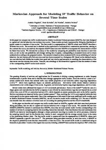
A. Model Validation To validate the hybrid priority network model, we consider a small example of two machine groups and four stages as depicted in Figure 4. Figure 5 shows the cycle times obtained by the hybrid SDA+QNA algorithm over the example. Although there exist difference in standard deviation for priority 2, the difference does not increase as the number of nodes increases. Numerical experiments are also conducted on a simple but full-scale fab model [6] to examine the efficiency, accuracy and application potential of the hybrid decomposition approximation-based queueing network modeling. Discrete event simulations are also developed for validation of the fab behavior model. The fab example has two parts with two priorities classes, and the numbers of processing steps of products P1 and P2 are 32 and 60, respectively. In a special fab model (SFM), all the service times of a node have exponential distributions. Details of SFM data are listed in Appendix A. Node and system level cycle times of the SFM are given in Figure 6, Figure 7, and Table 1 respectively. The differences of mean cycle times of two priorities and the cycle time standard deviation of P2 are mostly within 3%. Although the difference of cycle time standard deviation of P1 is high (up to 45%), the absolute error is only 1.627. In a general fab model (GFM), the service times of individual nodes have general distributions, such as uniform, erlang and exponential (see Appendix A). Node and system level cycle times of the GFM are given in Figure 8, Figure 9, and Table 2 respectively. The differences of mean cycle times of two priorities and the cycle time standard deviation of P2 are mostly within 10%. The cycle time standard deviation of P1 has a high relative error of 55%. But again, the absolute error, 1.214, is still very small as compared to the mean. Comparisons of numerical results with simulation in these two fab models show that our network modeling methodology provides good approximations in most nodal performances B. Model Tuning To further fit the decomposition-based priority queueing network model to the actual priority system and reduce the difference caused by approximation, we design a model tuning step for the behavior model. In the hybrid SDA+QNA model, the mean cycle time of one priority job consists of the mean waiting time and the service time, where the waiting time is divided into queueing and the approximate server vacation time because of higher priority jobs as given in Eq. (14). Consider the cycle time performance of priority 1. Figure 8 shows that the hybrid SDA+QNA provides a good approximation. But for priority 2, Figure 9 shows that there are positive errors in mean cycle times. We reason that the potential source of error to priority 2 is caused by the estimation of vacation time. So we use two parameters and for each machine group to compensate

the mean and variance of the vacation time in Eqs. (9) and (11) respectively. Take node 5 and node 12 for example. By adjusting the parameters of vacation time, the PCT approximation errors are reduced and lead to a close fit of the cycle time of priority 2 as compared to simulation results listed in Table 3. C. Computation Efficiency Application of hybrid decomposition approximation to each model (listed in Table 4) only requires less than 4 seconds of CPU time on a 2.8 GHz personal computer. This leads to fast calculation with respect to changes of system input options. Consequently, both the accuracy and computing efficiency of hybrid decomposition approximation-based network modeling support its potential for applications of real fab with service differentiation. IV.

CONCLUSIONS

Responding to rapidly changing complex SSC requirements, SSC planners/managers need an effective performance evaluation/prediction tool to do what-if analysis between SSC inputs and outputs. Given a set of priority mix, capacity, mean and variability of wafer release, mean service time and variability of tools, the hybrid decomposition approximation-based network model allows very quick evaluation of mean and variability of nodal and fab performance metrics with good accuracy. Effective evaluation of various input options in terms of capacity allocation, priority mix, wafer release policy, tool adjustment, etc., may serve as a behavior model for SSC performance optimization. The mean and variability statistics at individual tool groups may also be utilized by six-sigma management for on time and quick delivery, where the mean values can be used to derive control targets while variability values for calculation of control limits. ACKNOWLEDGEMENT This work was supported in part by the Semiconductor Research Corporation and International Semiconductor Manufacturing Initiative under FORCe-II project 1214 and by the National Science Council, Taiwan, R.O.C., under grant NSC95-2221-E-002-346-MY3.

Figure 1: Semiconductor supply chain

SDA+QNA

Priority 2 Mean Cycle Time

Hours

QNA

Simulation

14 12

Node m

SDA

Node n 10

P1 moving

1

1

2

2

P1 moving

8 6

P2 moving

P2 moving

4 2 0

Figure 2: Decomposition approximation-based queueing network modeling

1

2

3

4

5

6

7

8

9

10

11

12

Node Index

Figure 7: Mean cycle times of P2 in SFM nodes SDA+QNA

Priority 1 Mean Cycle Time

Hours

Simulation

2.4 2.1

Figure 3: Decomposition among priorities

1.8 1.5 1.2 0.9 0.6 0.3 0 1

2

3

4

5

6

7

8

9

10

11

12

Node Index

Figure 8: Mean cycle times of P1 in GMF nodes Figure 4: Two stations with reentrant line SDA+QNA

Priority 2 Mean Cycle Time

Hours

Simulation

10 SDA+QNA 1 SDA+QNA 2 Simulation 1 Simulation 2

Mean Cycle Time

Unit Time 600

Cycle Time Standard Deviation

Unit Time 280

SDA+QNA 1 SDA+QNA 2 Simulation 1 Simulation 2

6

200

400

5

160 300

4

120 200

3

80 100

2

40

0

1

0 2

3

4

8 7

240

500

9

5

2

3

Number of Nodes

4

Number of Nodes

Figure 5: Mean and standard deviation of cycle time for multi-nodes (2~5) with reentrant line

5

0 1

2

3

4

5

6

7

8

9

10

11

12

Node Index

Figure 9: Mean cycle times of P2 in GMF nodes SDA+QNA

Priority 1 Mean Cycle Time

Hours

Simulation

3 2.5 2 1.5 1 0.5 0 1

2

3

4

5

6

7

8

9

10

11

12

Node Index

Figure 6: Mean Cycle Times of P1 in SFM Nodes

Table 1: System level performance comparisons (SFM) Cycle Time Mean Cycle Time Standard Deviation SDA+QNA 18.613 5.190 Simulation 18.572±0.014 3.5622±0.008 1 Absolute Error 0.041 1.627 Relative Error 0.22 % 45.68 % SDA+QNA 172.78 54.674 Simulation 174.695±1.159 53.088±0.899 2 Absolute Error -1.915 1.586 Relative Error -1.10 % 2.99 %

Table A1: Service processes of nodes for special fab model Table 2: System level performance comparisons of general Cycle Time Mean Cycle Time Standard Deviation SDA+QNA 15.137 3.503 Simulation 15.451±0.009 2.289±0.005 1 Absolute Error -0.314 1.214 Relative Error -2.03 % 53.02 % SDA+QNA 122.22 36.392 Simulation 112.015±0.668 38.133±0.424 2 Absolute Error 10.205 -1.740 Relative Error 9.11% -4.56% Table 3: PCT adjustment table Machine





5 12

3.2 -1.6

-3.2 -1.6

P2 Modified Cycle time Approx. 8.4268 5.2404

Simul.

error

8.4102 5.2204

0.20% 0.38%

Appendix A: Fab Model Data 1 1 1 1 1 1 1

      

2 2 2 2 2 2 2

      

10 3 10 11 3 3 6

      

8  5 8 8 2

   

2  10 

3 

9 

12 

           

2 2 2 2 6 2 2 6 2 2 2 2

           

3  6  3  3  11  3  3  11  3  4  7  12 

8 

10 

8  8  1  8  8  1  8  8  8  Exit

9  10  2  9  10  2  9  3  10 

1 2

1 1

Exponential Exponential

3 4 5

1 1 1

Exponential Exponential Exponential

6 7 8

1 1 1

Exponential Exponential Exponential

9 10 11

1 1 1

Exponential Exponential Exponential

12

1

Exponential

MPT (hr/lot)

Utilization %*

0.125 0.125 0.25

88.38 85.23 91.54

1.8 0.9 0.6

68.18 90.91 83.33

1.8 0.2 0.6

68.18 80.81 83.33

0.3333 0.6 1.25

88.38 83.33 78.91

Node

# of Machines

Service Time Distribution

1 2

1 1

Erlang Order 4 Exponential

3 4 5

1 1 1

Uniform Erlang Order 3 Erlang Order 2

6 7 8

1 1 1

Erlang Order 4 Exponential Erlang Order 3

9 10 11

1 1 1

Uniform Erlang Order 2 Exponential

12

1

Uniform

MPT (hr/lot)

Utilization %*

0.125 0.125 0.25

88.38 85.23 91.54

1.8 0.9 0.6

68.18 90.91 83.33

1.8 0.2 0.6

68.18 80.81 83.33

0.3333 0.6 1.25

88.38 83.33 78.91

REFERENCES E xit

[1]

[2] 1 1 1 1 1 1 1 1 1 1 1 1

Service Time Distribution

8 

Figure A1: Process flow of P1 in 2-PR fab model Enter 

# of Machines

Table A2: Service processes of nodes for general fab model

Table 4: Comparisons of CPU times in fab models Average CPU time (seconds) Two Priorities Hybrid SDA+QNA Simulation (one run) Fab Models Special case 3.606 2466 General case 3.622 2484

E nter 

Node

[3] [4] 5  5  10 

[5] 11 

Figure A2: Process flow of P2 in 2-PR fab model

[6]

D. P. Connors, G. E. Feigin, and D. D. Yao, “ A Queueing network Model for Semiconductor Manufacturing,”IEEE Trans. Semi. Manuf., vol. 9, pp.412-427, 1996. G. Horvath and M. Telek,“ Ap pr o x i ma t e Ana l y s i so fPriority Queues,”Technical Report, Technical University of Budapest, 2000. W. Whitt, “ The Queueing Network Analyzer,”The Bell System Technical Journal, Vol. 62, pp2779-2815, 1983. M. D. Hu, S. C.Cha ng ,“ Tr a ns l a t i ngOv e r a l lPr o duc t i o nGoals into Distributed Flow Control Parameters for Semiconductor Manufacturing,”Journal of Manufacturing Systems, Vol. 22, No. 1, 46-63, 2003. J. D. Faires, and R.L. Burden, Numerical Methods, 3rd ed., Brooks/Cole Pub. Co., Nov. 2002. S. H. Lu, D. Ramaswamy, and P. R. Kumar, “ Ef f i c i e ntSc he dul i ng Policies to Reduce Mean and Variance of Cycle-Times in Semiconductor Manufacturing Plants,” IEEE Transactions on Semiconductor Manufacturing, Vol. 7, No. 3, August 1994.