Priority Queues, Pairing and Adaptive Sorting Amr Elmasry Computer Science Department, Rutgers University, New Brunswick, NJ 08903
[email protected]
Abstract. We introduce Binomialsort, an adaptive sorting algorithm that is optimal with respect to the number of inversions. The number of comparisons performed by Binomialsort, on an input sequence of length n that has I inversions, is at most 2n log nI + O(n) 1 . The bound on the number of comparisons is further reduced to 1.89n log nI + O(n) by using a new structure, which we call trinomial queues. The fact that the algorithm is simple and relies on fairly simple structures makes it a good candidate in practice.
1
Introduction
In many applications the lists to be sorted do not consist of randomly distributed elements, but are already partially sorted. An adaptive sorting algorithm benefits from the existing presortedness in the input sequence. Mannila [10] formalized the concept of presortedness. He studied several measures of presortedness and introduced the concept of optimality with respect to these measures. One of the main measures of presortedness is the number of inversions in the input sequence [6]. The number of inversions is the number of pairs in the wrong order. More precisely, for an input sequence X of length n, the number of inversions is defined Inv(X) = |{(i, j) | 1 ≤ i < j ≤ n and xi > xj }|. We assume that xi is to the left of xj , whenever i is less than j. For an adaptive sorting algorithm to be optimal with respect to the number of inversions, its running time should be in O(n log Inv(X) + n) [5]. n Finger trees [5, 2, 12] was the first data structure that utilizes the existing presortedness in the input sequence. Using a finger tree, the time required to sort a sequence X of length n is O(n log Inv(X) + n). The fact that the underlying n data structure is pretty complicated, and requires a lot of pointer manipulations, makes these algorithms impractical. Mehlhorn [11] introduced a sorting algorithm that achieves the above bound, but his algorithm is not fully practical as well. Other algorithms which are optimal with respect to the number of inversions, include Blocksort [9] which runs in-place, and the tree-based Mergesort [14] which is optimal with respect to several other measures of presortedness. Among the sorting algorithms which are optimal with respect to the number of 1
We define log x to be max(0, log2 x)
inversions, Splitsort [7] and adaptive Heapsort [8] are the most promising from the practical point of view. Both algorithms require at most 2.5n log n comparisons. Splaysort, sorting by repeated insertion in a splay tree [15], was proved to be optimal with respect to the number of inversions [3]. Moffat et al. [13] performed experimental results showing that Splaysort is practically efficient. See [4] for a nice survey of adaptive sorting algorithms. We introduce Binomialsort, an optimal sorting algorithm with respect to the number of inversions. The number of comparisons performed by Binomialsort + O(n). Next, we introduce trinomial queues, an alteris at most 2n log Inv(X) n native to binomial queues, and use it to reduce the bound on the number of comparisons performed by the algorithm to 1.89n log Inv(X) + O(n). The fact n that our algorithm is simple and uses simple structures makes it practically efficient, while having a smaller constant, for the leading term of the bound on the number of comparisons, than other known algorithms. The question about the existence of a selection sort algorithm, that uses a number of comparisons that + O(n), is open. matches the information theoretical lower bound of n log Inv(X) n
2
Adaptive transformations on binomial queues
A binomial tree [1, 16] of rank r is constructed recursively by making the root of a binomial tree of rank r − 1 the rightmost child of the root of another binomial tree of rank r − 1. A binomial tree of rank 0 consists of a single node. The following properties follow from the definition: – The rank of an n-node (assume n is a power of 2) binomial tree is log n. – The root of a binomial tree, with rank r, has r sub-trees each of which is a binomial tree, having respective ranks 0, 1, . . . , r − 1 from left to right. – Other than the root, there are 2i nodes with rank log n − i − 1, for all i from 0 to log n − 1. A binomial queue is a heap-ordered binomial tree. It satisfies the additional constraint that every node contains a data value smaller than or equal to those stored in its children. We use a binary implementation of binomial queues. In such an implementation, every node has two pointers, One pointing to its right sibling and the other to its rightmost child. The right pointer of a rightmost child points to the leftmost child to form a circular list. Given a pointer to a node, both its rightmost and leftmost children can be accessed in constant time. The list of its children can be sequentially accessed from left to right. Given a forest F , each node of which contains a single value, the sequence of values obtained by a pre-order traversal of F is called the corresponding sequence of F and denoted by P re(F ). Our traversal gives precedence to the trees of the forest in left-to-right order. Also, the precedence ordering of the sub-trees of a given node proceeds from left to right. A transformation on F that results in a forest F 0 shall be considered Inv-adaptive provided that
Inv(P re(F 0 )) ≤ Inv(P re(F )). Our sorting algorithm will be composed of a series of Inv-adaptive transformations, applied to an initial forest consisting of a sequence of singleton-node trees (the input sequence). The idea is to maintain the presortedness in the input sequence, by keeping the number of inversions in the corresponding sequence of the forest non-increasing with time. The following transformations are needed throughout the algorithm: Heapifying binomial queues Given an n-node binomial queue, T , such that the value at its root is not the smallest value, we want to restore the heap property. Applying the standard heapify operation will do. Moreover, this transformation is Inv-adaptive. Recall that the heapify operation proceeds by finding the node, say x, with the smallest value among the children of the root and swapping its value with that of the root. This step is repeated with the node x as the current root, until either a leaf or a node that has a value smaller than or equal to all the values of its children is reached. To show that the heapify operation is Inv-adaptive, consider any two elements xi , xj ∈ P re(T ), where i < j. If these two elements were swapped during the heapify operation, then xi > xj . Since xi appears before (to the left of) xj in P re(T ), we conclude that this swap decreases the number of inversions. It remains to investigate how the heapify operation is implemented. Finding the minimum value within a linked list requires linear time. This may lead to an O(log2 n) time for the heapify operation. We can do better, however, by maintaining with every node an extra pointer that points to the node with the smallest value among all its left siblings, including itself. We call this pointer, the pointer for the prefix minimum (pm). The pm pointer of the rightmost child of a node will, therefore, point to the node with the smallest value among all the children of the parent node. To maintain the correct values in the pm pointers, whenever the value of a node is updated all the pm pointers of its right siblings, including itself, have to be updated. This is accomplished by proceeding from left-to-right; the pm pointer of a given node, x, is updated to point to the smaller of the value of x and the value of the node pointed to by the pm pointer of the left sibling of x. A heapify at a node with rank r1 reduces to a heapify at its child with the smallest value whose rank is r2, after one comparison plus at most r1 − r2 comparisons to maintain the pm pointers. Let H(r) be the number of comparisons used by the above algorithm to heapify a binomial queue whose root has rank r, then H(0) = 0,
H(r1 ) ≤ H(r2 ) + r1 − r2 + 1.
The number of comparisons is, therefore, at most 2 log n. The number of comparisons can still be reduced as follows. First, the path from the root to a leaf, where every node has the smallest value among its siblings, is determined by utilizing the pm pointers. No comparisons are required for this step. Next, the value at the root is compared with the values of the nodes
of this path bottom up, until the correct position of the root is determined. The value at the root is then inserted at this position, and all the values at the nodes above this position are shifted up. The pm pointers of the nodes whose values moved up and those of all their right siblings are updated. The savings are due to the fact that at each level of the queue (except possibly for the level of the final destination of the old value of the root), either a comparison with the old value of the root takes place or the pm pointers are updated, but not both. Then, the number of comparisons is at most log n + 1. In the sequel it is to be understood that our binomial queues will be augmented with pm pointers as described above. Lemma 1. The number of comparisons needed to heapify an n-node binomial queue is at most log n + 1. Inv-adaptive construction of binomial queues Given an input sequence of length n, we want to build a corresponding binomial queue Inv-adaptively. This is done by recursively building a binomial queue with the rightmost n2 elements, and another binomial queue with the leftmost n2 elements. The root of the right queue is linked to the root of the left queue as its rightmost child. If the value at the root of the right queue was smaller than the value at the root of the left queue, the two values are swapped. A heapify operation is then called to maintain the heap property for the right queue, and the pm pointer of the root of the right queue is updated. Note that swapping the values at the roots of the two queues is an Inv-adaptive transformation. Let B(n) be the number of comparisons needed to build a queue of n nodes as above, then n B(2) = 1, B(n) ≤ 2B( ) + log n + 2. 2 Lemma 2. Given an input sequence of length n, a binomial queue can be Invadaptively built with less than 3n comparisons. Proof. Consider the recursion tree corresponding to the above recursive relations. There are 2ni nodes each representing a sub-problem of size 2i , for all i from 2 to log n. The number of comparisons associated with each of these subproblems is two plus the logarithm of the size of the sub-problem, for a total of Plog n n n i=2 (i+2) 2i < 2.5n. Also, there are 2 sub-problems each of size 2, representing the initial conditions, for a total of another n2 comparisons. Note that, a bound of 2.75n can be achieved by replacing the initial condition with B(4) = 5. t u
3
Adaptive pairing
For any two queues q1 and q2 , where q1 is to the left of q2 , a pairing operation is defined as follows. If the value of the root of q2 is the smaller, perform a left-link by making q1 the leftmost child of the root of q2 . Otherwise, perform a right-link by making q2 the rightmost child of the root of q1 . See Fig. 1. It is
straightforward to verify that this way of pairing is Inv-adaptive. Consider the corresponding sequence of the heap before and after the pairing. This sequence will not change by a right-link. A left-link changes the position of the root of the right queue, by moving it before (to the left of) all the elements of the left queue. Since the value of the root of the right queue is smaller than all the elements of the left queue, the number of inversions of the corresponding sequence decreases. The Inv-adaptive property follows. Given a forest of priority queues, we combine these queues into a single queue as follows. Starting from the rightmost queue, each queue is paired with the result of the linkings of the queues to its right. We refer to this right-toleft sequence of node pairings as a right-to-left incremental pairing pass. The intuition behind doing the pairing from right to left is to keep the number of right-links throughout the algorithm linear, as will be clear later.
4
The Binomialsort algorithm
Given an input sequence X of length n. If n is not a power of 2 we split the input list into sub-lists of consecutive elements whose lengths are powers of 2. The lengths of the sub-lists have to be strictly increasing from left to right. Note that this splitting is unique. The sorting algorithm is then applied on each sublist separately. We then do a merging phase to combine the sorted sub-lists. We start with the leftmost (shortest) two sub-lists and merge them. Then, the result of the merging is repeatedly merged with the next list to the right (next list in size), until all the elements are merged. Lemma 3. The number of comparisons spent in merging is less than 2n. Proof. Let the lengths of the k sub-lists from left to right be 2j1 , 2j2 , . . . 2jk , where j1 < j2 < . . . < jk . Let Ci be the number of comparisons needed toPmerge the i leftmost i sub-lists, where i ≤ k. We prove by induction that Ci < l=1 2jl +1 . P i The base case follows, since C2 < 2j1 + 2j2 . We also have Ci < Ci−1 + l=1 2jl . Pi−1 jl +1 Pi jl Assuming the hypothesis is true for i−1, then Ci < l=1 2 + l=1 2 . Using Pi−1 jl Pi−1 jl +1 ji ji +1 +2 , and the hypothesis the fact that l=1 2 < 2 , then Ci < l=1 2 Pk t u is true for all i. Since n = l=1 2jl , then Ck < 2n.
Throughout the algorithm, we assume without loss of generality that n is a power of 2. The algorithm in a nutshell is: Build an initial binomial queue Inv-adaptively. While the heap is not empty do Delete the root of the heap and output its value. Do a fix-up step. Do a right-to-left incremental pairing pass. enddo To implement the fix-up step efficiently, we associate a pseudo-rank with every node. This rank field may be different from the natural rank defined in Sect. 2 for binomial queues. After building the initial binomial queue, the pseudo-rank of every node is equal to its natural rank. Consider any node, x, the first time it becomes a root of a tree immediately before a pairing pass. Define to-the-left(x) to be the set of nodes of the trees to the left of the tree of x, at this moment. Note that, before this moment, to-the-left(x) is not defined. The following invariant must hold throughout the algorithm: Invariant 1. The pseudo-rank of any node, x, must be strictly greater than the pseudo-rank of all the nodes in to-the-left(x). For a given node, call the children that were left-linked to that node, the L-children. Call the, at most one, child that may be right-linked to that node, the R-child (We will show later that, as a result of our pairing strategy, any node may gain at most one right child). And call the other children the I-children. The following two properties, concerning the children of a given node, are a direct consequence of Invariant 1: Property 1. The R-child is the rightmost child and its pseudo-rank is the largest pseudo-rank among its siblings and parent. Property 2. The pseudo-ranks of the L-children are smaller than that of their parent. Moreover, they form an increasing sequence from left to right. If the pseudo-rank of the root of a binomial queue is equal to its natural rank, this binomial queue is a heavy binomial queue. If the pseudo-rank of this root is one more than its natural rank, the binomial queue is a light binomial queue. The number of nodes of a light binomial queue, whose pseudo-rank is r, is 2r−1 . We call the root of a light binomial queue, a light node. All other nodes are called normal nodes. The special case of a light binomial queue with pseudo-rank 0 is not defined. In other words, a binomial queue with pseudo-rank 0 is a single node, and is always heavy. Invariant 2.1. The I-children of a normal node, whose pseudo-rank is r, are the roots of heavy or light binomial queues. The pseudo-ranks of these I-children, from left to right, form a consecutive sequence from 0 up to either r − 1 or r.
Invariant 2.2. Immediately before the pairing pass, all the roots of the queues are normal nodes. For the initial binomial queue, all the children are I-children, and both Invariant 1 and Invariant 2 hold. When time comes for a node to leave the heap, the pseudo-ranks of its children form at most two runs of strictly increasing values from left to right. One is formed from the L-children, and the other is formed from the I-children and the R-child. The purpose of the fix-up step is to reconstruct such a forest of queues to form one single run of increasing pseudo-ranks from left to right, while maintaining Invariant 1 and Invariant 2. Subsequent to the initial construction of the binomial queue, the pseudo-ranks are updated during the fix-up step as illustrated below. The fix-up step Let w be the node that has just been deleted before the fix-up step. We start with the leftmost queue and traverse the roots of the queues from left to right, until a node whose pseudo-rank is greater than or equal to the pseudo-rank of its right neighbor is encountered (if at all such a node exists). Call this node x and its pseudo-rank rx . This node must have been the first L-child linked to w, and its right neighbor must be the leftmost I-child (By Invariant 2, this queue is a single node whose pseudo-rank is 0). Property 2 implies that, before w leaves the heap, its pseudo-rank must have been strictly greater than rx . Property 1 implies that if w has an R-child, the pseudo-rank of this child must be greater than rx + 1. Starting from the right neighbor of x, we continue traversing the roots of the queues from left to right, while the pseudo-ranks of the traversed nodes are less than or equal to rx + 1. Call the forest of queues defined by these nodes the working-forest. The above analysis implies that the roots of the queues of the working-forest are I-children of w. Invariant 2 implies that the pseudo-rank of the root of the rightmost queue of the working-forest is either rx or rx + 1. A trivial case arises if there is only one queue in the working forest. By Invariant 2, The pseudo-rank of this node, y, must be 0. This implies that rx is equal to 0, and x is a single node as well. The fix-up step, in this case, ends by making the node that has the smaller value of x and y, the parent of the other node, and assigning a pseudo-rank 1 to it. If the number of queues of the working-forest is more than one, we perform a combine step. a) Combine. The combine starts by promoting the single node queue representing the leftmost queue of the working forest, giving it a pseudo-rank of rx + 1, and making it the root of the combined queue. In other words, we make the other roots of the queues of the working-forest I-children of this promoted node. The binomial queues of the working forest are traversed from left to right, until a heavy binomial queue, say h, is encountered. The pseudo-rank of the root of each of the light binomial queues, to the left of h, is decreased by 1, making these binomial queues heavy. Let rh be the pseudo-rank of the root of h. We
proceed by splitting h into two binomial queues; the right queue is the queue whose root was the rightmost child of the root of h before the split, while the rest of h form the left queue. The left binomial queue is assigned a pseudo-rank rh − 1, indicating that it is a heavy binomial queue, while the right binomial queue is assigned a pseudo-rank rh , indicating that it is a light binomial queue. After this step, the pseudo-ranks of the roots of the queues of the working-forest still form a consecutive sequence from left to right, and Invariant 2.1 holds. Note that this process is similar to subtracting 1 from the binary representation of an integer. Finally, perform a heapify operation on the combined queue. See Fig. 2. It is straightforward to verify that the combine step is Inv-adaptive. Consider the case where all the queues of the working-forest are light queues. The pseudo-rank of the root of each of these queues is decreased by 1, making it a heavy binomial queue. If the pseudo-rank of the root of the rightmost queue was rx and now becomes rx − 1, for Invariant 2 to hold, the promoted root is assigned a pseudo-rank rx , instead of rx +1, and a fusion step is to be performed.
b) Fusion. If the pseudo-rank of the root of the combined queue is rx , a fusion step is performed. Call the root of the combined queue y. The way the combine step is done insures that the combined queue, in this case, is a binomial queue. The queue of y is fused with the queue of x as follows. If the value of y is smaller than the value of x, the two values are swapped and a heapify step is performed on the queue of y. The pseudo-rank of x is incremented by 1. Let z be the rightmost child of x and its pseudo-rank rz . If rz < rx , the fusion ends by making the queue of y the rightmost I-child of x. In this case, Invariant 2 implies rz = rx − 1, and Invariant 2.1 still holds after the fusion. Otherwise (rx = rz , a
case that happens only if x was promoted in a previous combine step), the value of y is compared with the value of z. If the value of y is smaller, the two values are swapped and a heapify step is performed on the queue of y. The queue of y becomes the rightmost I-child of z, and the pseudo-rank of z is incremented by 1. Since the queue of y is a binomial queue, Invariant 2.1 again holds in this case. See Fig. 3 for an example. Since the heapify operation is Inv-adaptive, it follows that the fusion step is Inv-adaptive as well.
c) Gluing. The last step of the fix-up is to maintain Invariant 2.2. The roots of the queues are traversed from left to right, searching for light nodes. Light nodes may have been I-children of w, that were not included in the combined queue of the working forest. When a light node is encountered its rank is decreased by 1, making it a normal node. We may now face another problem; Invariant 1 may no longer be true, since there may be two sibling nodes having the same rank. The first observation is that, for a given rank, there may be at most two roots that have this rank. The second observation is that the queues of any two roots having the same rank must have been one queue, which was split by a combine step at some point of the algorithm. This follows from the fact that the right queue, among any of these pairs, was a light queue, indicating that it was split in a previous step of the algorithm. Each pair of such queues is glued together by making the right queue the rightmost child of the root of the left queue, and increasing the rank of the root of the glued queue by 1. Note that, during the gluing step, no comparisons are performed between the values of the nodes. Analysis Lemma 4. The number of right-links in all the pairing passes is less than n.
Proof. The right-to-left incremental pairing pass ensures that a node can gain at most one R-child. When a node gains an R-child it becomes the root of the rightmost queue. From this point on this node will never have a right sibling and will always be a node on the right spine of the rightmost queue. Hence, it will never gain another R-child in any pairing pass. t u Lemma 5. The number of comparisons involved in all the fusion steps is at most 2n. Proof. Consider a fusion step between any two queues q1 and q2 , where q1 is to the left of q2 . Let r be the pseudo-rank of the roots of the two queues before the fusion. The first observation is that q2 must be a binomial queue. During the fusion, in the worst case, one comparison and a heapify step are performed on q2 , at most twice. Therefore, the number of comparisons involved is at most 2 when r = 0, at most 4 when r = 1, and at most 2(r + 2) in general. What makes the overall comparisons, performed during fusion steps, linear is that fusion steps are not executed in most of the iterations of the algorithm. More precisely, Before this fusion step, there should have been 2r nodes that have already left the heap without executing a fusion step, and can be associated only with this fusion step. (Each of these 2r nodes must have left the heap with a combine step that was not followed by a fusion step.) For more illustration, consider the nodes of q2 . In the previous iteration of the algorithm, these nodes were descendents of a root whose pseudo-rank was at least r + 1. The last time the queue that contains these nodes may have been involved in a fusion step (as a right queue) was when it was a heavy binomial queue, i.e. it had 2r+1 descendents. From this point, a total of 2r nodes, of the descendents of this queue, have left the heap, and each time the fix-up did not include a fusion step. We charge each of these 2r nodes twice. Since, for all values of r, 2r+1 credits cover the cost of the current fusion step, the lemma follows. t u Lemma 6. The pseudo-rank of a normal node, that has s descendants, is less than log s + 1. Proof. Let r be the pseudo-rank of a normal node that has s descendents. To establish a lower bound on s, we use Invariant 2. The node itself contributes 1 to s. Consider the I-children of this node. The leftmost I-child is a single node. The other children are roots of binomial queues whose pseudo-ranks form a consecutive sequence from 1 to either r−1 or r. Even if these binomial Pr−2 queues are light, they contribute at least 20 , 21 , . . . , 2r−2 to s, then s ≥ 2+ i=0 2i > 2r−1 .u t Lemma 7. The number of comparisons involved in the heapify operations in all + 3n. the combine steps is less than n log Inv(X) n Proof. Consider the moment when a node w is leaving the heap. Let fw be the number of descendents of the L-children of w. Each of these nodes represents an element that is greater than w and was appearing before (to the left of) w in the input sequence. Since all the steps ofPthe algorithm are Inv-adaptive, taking the summation over all the nodes, then x fx ≤ Inv(X).
Assume that the pseudo-rank of the first L-child gained by w is r. Using Lemma 6, then r < log fw + 1. During the combine step that follows the deletion of w, the accompanying heapify operation is performed on a queue whose pseudorank is at most r + 1, for a total of at most r + 2 comparisons. Let CH be the number of comparisons involved in all the heapify operations of the combine steps. Using Jensen’s inequality, and taking the summation over P + 3n. t u all the nodes of the heap, then CH < x (log fx + 3) ≤ n log Inv(X) n Lemma 8. The number of left-links in all the pairing passes is less than n log Inv(X) + n. n Proof. Consider the moment when a node w is leaving the heap. Let fw be as defined in Lemma 7. Let lw be the number of L-children of w. Using Property 2, andP applying Lemma 6 on each of the sub-trees defined by these nodes, then lw −1 i−1 fw > i=1 2 + 1, and hence lw < log fw + 1. Let L be the number of leftP links. Using Jensen’s inequality, then L < x (log fx + 1) ≤ n log Inv(X) + n. t u n The following theorem follows, as a consequence of the above lemmas. Theorem 1. Binomialsort sorts a sequence X of length n, in at most + O(n) comparisons and O(n log Inv(X) + n) time. 2n log Inv(X) n n
5
Trinomial queues
A trinomial tree of rank r is constructed recursively using 3 trinomial trees of rank r − 1. The first is linked as the rightmost child of the second. Then, the second is linked as the rightmost child of the third. A trinomial tree of rank 0 consists of a single node. The following properties hold for trinomial trees: (Assuming that the number of nodes n is a power of 3) – The rank of an n-node trinomial tree is log3 n. – The root of a trinomial tree, with rank r, has r children, having respective ranks 0, 1, . . . , r − 1 from left to right. – Other than the root, there are 2.3i nodes with rank log3 n − i − 1, for all i from 0 to log3 n − 1. A trinomial queue is a heap ordered trinomial tree. Applying the same techniques we used for heapifying binomial queues on trinomial queues, the number of comparisons needed to do the heapify on a trinomial queue of rank r is at most 2r + 1. In a similar fashion, building an initial trinomial queue Inv-adaptively can be done in linear time. A trinomial queue is considered heavy if the pseudo-rank of its root is equal to its natural rank. A light trinomial queue, with pseudo-rank r, consists of two heavy trinomial queues, with pseudo-ranks r − 1, one of them is the rightmost child of the other. This means that a light trinomial queue, with rank r, has 2.3r−1 nodes. During the combine step, when a heavy trinomial queue, with
pseudo-rank r, is split, its rightmost child becomes the right queue, which is a light queue with pseudo-rank r, and the rest of the queue becomes the left queue, which is a heavy queue with pseudo-rank r − 1. Using trinomial queues instead of binomial queues throughout the algorithm, it can be easily verified that the number of comparisons involved in all the heapify operations during the fix-up steps is at most log2 3 n log Inv(X) + O(n), and the n number of left-links is at most
Inv(X) 1 log 3 n log n
+ O(n). All the other operations
require a linear number of comparisons, for a total of at most O(n) comparisons.
Inv(X) 3 log 3 n log n
+
Theorem 2. Trinomialsort sorts a sequence X of length n, in at most 1.89n log Inv(X) + O(n) comparisons and O(n log Inv(X) + n) time. n n
References 1. M. Brown. Implementation and analysis of binomial queue algorithms. SIAM J. Comput. 7 (1978), 298-319. 2. M. Brown and R. Tarjan. Design and analysis of data structures for representing sorted lists. SIAM J. Comput. 9 (1980), 594-614. 3. R. Cole. On the dynamic finger conjecture for splay trees. Part II: The proof. SIAM J. Comput. 30 (2000), 44-85. 4. V. Estivill-Castro. A survey of adaptive sorting algorithms. ACM Comput. Surv. vol 24(4) (1992), 441-476. 5. L. Guibas, E. McCreight, M. Plass and J. Roberts. A new representation of linear lists. ACM Symp. on Theory of Computing 9 (1977), 49-60. 6. D. Knuth. The Art of Computer Programming. Vol III: Sorting and Searching. Addison-wesley, second edition (1998). 7. C. Levcopoulos and O. Petersson. Splitsort - An adaptive sorting algorithm. Information Processing Letters 39 (1991), 205-211. 8. C. Levcopoulos and O. Petersson. Adaptive Heapsort. J. of Alg. 14 (1993), 395-413. 9. C. Levcopoulos and O. Petersson. Exploiting few inversions when sorting: Sequential and parallel algorithms. Theoretical Computer Science 163 (1996), 211-238. 10. H. Mannila. Measures of presortedness and optimal sorting algorithms. IEEE Trans. Comput. C-34 (1985), 318-325. 11. K. Mehlhorn. Sorting presorted files. Proc. Of the 4th GI Conference on Theory of Computer Science. LNCS 67 (1979), 199-212. 12. K. Mehlhorn Data Structures and Algorithms. Vol. 1. Sorting and Searching. Springer-Verlag, Berlin/Heidelberg. (1984). 13. A. Moffat, G. Eddy and O. Petersson. Splaysort: fast, verstile, practical. Softw. Pract. and Exper. Vol 126(7) (1996), 781-797. 14. A. Moffat, O. Petersson and N. Wormald A tree-based Mergesort. Acta Informatica, Springer-Verlag (1998), 775-793. 15. D. Sleator and R. Tarjan. Self-adjusting binary search trees. J. ACM 32(3) (1985), 652-686. 16. J. Vuillemin. A data structure for manipulating priority queues. Comm. ACM 21(4) (1978), 309-314.