Article
Priority Queues with Fractional Service for Tiered Delay QoS Gary Chang *,† and Chung-Chieh Lee † Received: 28 October 2015; Accepted: 14 December 2015; Published: 29 December 2015 Academic Editor: Fernando Cerdán Department of EECS, Northwestern University, Evanston, IL 60201, USA;
[email protected] * Correspondence:
[email protected]; Tel.: +1-312-804-1731 † These authors contributed equally to this work.
Abstract: Packet scheduling is key to quality of service (QoS) capabilities of broadband wired and wireless networks. In a heterogeneous traffic environment, a comprehensive QoS packet scheduler must strike a balance between flow fairness and access delay. Many advanced packet scheduling solutions have targeted fair bandwidth allocation while protecting delay-constrained traffic by adding priority queue(s) on top of a fair bandwidth scheduler. Priority queues are known to cause performance uncertainties and, thus, various modifications have been proposed. In this paper, we present a packet queueing engine dubbed Fractional Service Buffer (FSB), which, when coupled with a configurable flow scheduler, can achieve desired QoS objectives, such as fair throughputs and differentiated delay guarantees. Key performance metrics, such as delay limit and probability of delay limit violation, are derived as a function of key FSB parameters for each delay class in the packet queueing engine using diffusion approximations. OPNET simulations verify these analytical results. Keywords: quality of service; modeling; simulation; diffusion approximation; broadband routers
1. Introduction Packet scheduling is central to high-speed routing networks that leverage statistical multiplexing of traffic flows to maximize bandwidth efficiency. In these networks, bandwidth contention arisen from traffic burstiness may result in occasional congestion at a packet router or a network access point. During periods of congestion, a well-designed packet scheduler is needed to allocate bandwidth to competing traffic flows from various classes of users and applications to maintain their required or contracted quality of service (QoS) levels, in terms of queuing delay, packet loss, or throughput. In this environment, QoS contracts can only be fulfilled with a non-zero probability of violation. A great deal of packet scheduling research has focused on fair allocation of bandwidth [1–4]. These contributions emphasize the throughput aspect of QoS and deal primarily with flow scheduling. In these cases, the scheduler essentially treats packets solely on the QoS status of their owner flows. One drawback of flow schedulers is that delays of individual packets are not accounted for and, thus, access delays for short-lived traffic flows are not protected. Furthermore, packet retransmissions may occur due to excessive packet delays even when the flow-level fairness is maintained. As Internet and mobile applications become increasingly bandwidth demanding and multimedia driven, maintaining fairness while providing protection for delay sensitive multimedia data plays an important role in modern network design and management. As packets associated with different traffic flows may have similar delay limits as determined by the flow scheduler, they can be grouped and treated equally as a delay class. One simple approach to differentiate delays between classes is to use priority queues. However, strict priority queues are known to cause highly uncertain delays on all classes except the highest. To provide meaningful packet delay
Future Internet 2016, 8, 1; doi:10.3390/fi8010001
www.mdpi.com/journal/futureinternet
Future Internet 2016, 8, 1
2 of 15
protections, every delay class must receive a certain fraction of service relative to the higher-priority classes to prevent starvation when higher priority classes present heavy loads. This notion of fractional service is the main motive of this work. We shall present a two-stage packet scheduling architecture that can be tailored to satisfy both flow-level throughput fairness and packet-level delay protections. The first stage is a buffer-less flow scheduler of which the responsibility is to classify packets based on their flow QoS. No specific flow QoS strategies will be assumed except that each classified packet is given a delay limit associated with its assigned delay class. The second stage is a packet queueing engine that uses as many buffers as delay classes to queue classified packets. Its responsibility is to protect the delay guarantee of each delay class such that it is met with a sufficiently high probability. This paper focuses on the second stage: the packet queueing engine. We shall present and analyze the packet queueing engine dubbed Fractional Service Buffer (FSB) that allows a fraction of lower-priority (higher-delay-limit) traffic class to advance their queueing priority at every higher-priority packet arrival. The fraction, in conjunction with the buffer size, determines a delay limit and a delay-violation probability associated with each delay class. Basically, our approach adds a fair queueing component to the conventional static priority queues, such that the lower-priority traffic may improve their priority over time and thus will not be shut out by higher-priority traffic. The rest of this paper is organized as follows. In Section 2, we cite some related literatures in flow scheduling and priority-queueing schemes. In Section 3, we present the two-stage FSB architecture and its fractional service algorithm. In Section 4, we analyze the FSB under heavy traffic conditions using a combination of queue aggregation technique and diffusion approximations. In Section 5, we demonstrate the accuracy of our analytical results from Section 4 using simulations. In Section 6, we discuss the relationship between the system parameters and desired QoS levels and how tradeoffs between different QoS levels can be achieved. In Section 7, we provide a concrete design example on tuning the FSB system parameters. 2. Related Works In terms of providing better packet delay for each traffic flow, the scheduler in [5] separates traffic flows with substantially different bandwidth requirements into different groups. Then, a time-stamp based scheduler is used to schedule the service of each group while a round-robin scheduler is used to service flows within a group. However, due to its round-robin structure, there is an inherit dependency between the allocated bandwidth of a flow and the queueing delay of the flow’s packets [6]. Furthermore, only the first packet of each flow can receive a delay protection. In [6], the authors presented a two-stage architecture that separates the dependencies between bandwidth allocations and packet delays. The first stage is a number of rate regulators that shape the traffic of each flow while the second stage is a number of strict priority queues that queue the regulated packets of each flow. Delay protections are achieved using an admission control policy that monitors the occupancy level at each priority queue. This implementation requires one buffer per flow to regulate each flow’s packets, in additional to the priority queues. These flow buffers require a separate management algorithm to ensure efficient usages of the memory space [7]. Class-based schedulers, on the other hand, have a far simpler approach in managing the memory space. In the Relative Differentiated service (RD) [8] framework, packets are grouped into M + 1 classes of service where Class-i packets receive better performance metrics than Class-i + 1 packets for all 0 ď i < M. One simple way of realizing RD is to use strict priority queues where the highest priority class is assigned to the highest priority queue and each queue is serviced in the order of their priority. However, such a method does not provide any means for adjusting the quality of each priority class and no delay protections can be offered to lower priority classes. In terms of overcoming the inflexibilities of strict priority queues, the authors of [8] presented a delay-ratio idea for determining service orders of each priority class. Specifically, they defined a delay ratio between every pair of service classes and the scheduler strives to maintain these service ratios
Future Internet 2016, 8, 1
3 of 15
at their target levels. In this manner, the relative service quality in terms of packet delays between classes is maintained, regardless of the load of higher-priority classes. The authors also applied their delay-ratio idea to existing queueing disciplines, such as Generalized Processor Sharing [9] and Waiting-Time Priority [10], to deliver controllable service qualities. This approach only offers a single dimension in QoS provisioning, namely the delay-ratio between classes. Separate mechanisms are required to ensure the fairness and maximum delay of each traffic class [11]. Other related literature, such as delay-dependent priority jumps [12], deals with this strict priority issue by prioritizing each packet based on its delay limit and tagging the packet with its entry time. The priority of a packet is increased if the maximum queueing delay of the packet in a priority queue is reached. This method requires tagging and updating timestamps of packets to accomplish priority increases. In [13], the authors presented several priority-jumping policies for systems with two priority classes. Each policy has a unique criterion for increasing the priority of lower priority packets. They concluded that each policy has its pros and cons and no single policy is a clear winner. The system that bases its priority increase criterion on the arrival of higher priority packets is the most “self-adaptive” to different traffic conditions. However, obtaining an exact analytical expression for this system is “extremely difficult”. 3. Fractional Service Buffers Although commonly referred to as “packet schedulers”, throughput-based schedulers are essentially flow schedulers. Examples of these include Deficit Round Robin (DRR) [14], Weighted Round Robin (WRR), and Weighted Fair Queueing (WFQ) [9] schedulers. However, throughput contracts are meaningful for traffic flows rather than individual packets. Service order of packets is determined solely by flows’ QoS attributes in a flow scheduler. Typically, a flow scheduler uses one queue for each active traffic flow and serves these flow queues with a scheduling discipline to fulfill their throughput contracts. In any of these scheduling solutions, packet delays of a given traffic flow vary with the flow’s packet arrival pattern and the overall system load. As a result, while the throughput of a traffic flow is protected, individual packet delays are not. For short traffic flows, the throughput may not be a meaningful QoS metric since their durations are just a few packets. The quality of these short flows’ services is better represented by their packet delays. Because the majority of traffic flows in the Internet are short [15], packet delays of these flows are a critical contributor to user experience. Furthermore, in a TCP dominated network environment, excessive packet delays may lead to TCP retransmissions thus increasing the duration of congestion. We are presenting a two-stage packet scheduling architecture where the first stage schedules traffic flows and the second stage protects packet delays. In Figure 1, a buffer-less flow scheduler classifies each input packet into a delay class based on its owner flow’s QoS status, while a subsequent packet queueing engine strives to protect the delay limit associated with each class. The flow scheduler maintains flow throughput by specifying a delay limit on each packet. For example, suppose the flow scheduler classifies packets by using a token bucket mechanism with load-adaptive token rates. Instead of physically maintaining a token bucket for each flow in the flow scheduler, the flow scheduler can simply compute the delay limit of each incoming packet based on its flow’s token rate and its available tokens, if any. The packet is mapped accordingly to a delay class based on its delay limit and then sent to the packet queueing engine. Actual packet delay will not reach the specified delay limit unless the system is fully loaded. As such, flows will likely receive more bandwidth than specified by the token bucket algorithm.
can simply compute the delay limit of each incoming packet based on its flow’s token rate and its available tokens, if any. The packet is mapped accordingly to a delay class based on its delay limit and then sent to the packet queueing engine. Actual packet delay will not reach the specified delay limit unless the system is fully loaded. As such, flows will likely receive more bandwidth than specified by Future Internet 2016, 8, 1 4 of 15 the token bucket algorithm.
1. Two-stage packet scheduling architecture. FigureFigure 1. Two-stage packet scheduling architecture.
The simple token bucket algorithm mentioned above for the flow scheduler is merely an example of associating flow throughputs with packet delays. Advanced algorithms, such as WFQ, WF2 Q [14] and Least Attained Service [15], which map flow throughputs into packet delays, are also suitable candidates. A flow scheduling policy, in conjunction with the delay protection provided by the packet queueing engine, provides configurable parameters for network operators to tune the desired level of QoS. The key in a configurable QoS scheduler is the packet queueing engine that offers multiple classes of delay protections, where the delay protection of each class can be quantified based on the traffic parameters given by a flow scheduling policy and an admission control policy. In this paper, we are leaving open the flow scheduling policy while assuming that the flow scheduler assigns each packet a delay class according to some selected flow QoS principles. We shall focus on the design and analysis of the packet queueing engine, dubbed the Fractional Service Buffers (FSB), of which the objective is to deliver the packet delay limit of each delay class. The FSB employs M + 1 FIFO buffers, dubbed Buffer-0, Buffer-1, . . . , Buffer-M, to accommodate M + 1 classes of classified packets. An arriving Class-i packet is placed in Buffer-i so long as this does not result in a buffer overflow. Basically, Class-0 corresponds to the most delay-sensitive packets and Class-M the least delay-sensitive packets as determined by the flow scheduler. A Class-i packet has a delay limit τi to be protected by the FSB, where τ0 < τ1 < . . . < τ M . Strict priority queues can be used to differentiate service qualities of multiple classes of traffic. However, strict priority queues, by itself, cannot protect the throughput or the delay of lower-priority classes when higher-priority classes present heavy traffic. Furthermore, the relative service level between traffic classes cannot be quantified or adjusted. The FSB serves its buffers in a strict priority order as well, but it employs a fractional service algorithm (FSA) to “move” packets between buffers in a controlled fashion thus achieving delay guarantees. In the FSB, Class-0 has the highest service priority while Class-M the lowest. Buffer-i earns a unit fractional credit whenever there is a packet arrival from the flow scheduler at ANY of the higher-priority buffers, i.e., Buffer-0, Buffer-1, . . . Buffer-(i ´ 1). Once the credit accumulates to one full credit, the packet at the head of Buffer-i is “moved” to Buffer-(i ´ 1). The credit balance of Buffer-i is then reset to zero. While packet sizes may be used to determine flow fairness in the flow scheduler, packets of different sizes are treated equally by the FSB. We will elaborate on how the FSA moves packets between queues such that a lower-priority class effectively shares a fraction of service with its higher-priority counterpart. The FSB maintains a credit counter for each buffer except Buffer-0. For every packet arriving at Buffer-i, each lower-priority buffer, Buffer-(i + k), 1 ď k ď M ´ i, receives a unit fractional credit of ηi`k = 1/(m(i + k)), regardless of the size of the arriving packet. In other words, Buffer-i receives a credit 1/(mi) whenever a packet arrives at one of the buffers with a priority higher than i (i.e., Buffer-0, Buffer-1, . . . , Buffer-(i ´ 1)). The integer m is a configurable parameter used to control the unit fractional credit. When the credit accumulated by Buffer-i reaches unity, its leading packet is moved to Buffer-(i ´ 1) and is thus “promoted” to Class-(i ´ 1). A promoted packet is treated equally as any other newly arriving packets to that class. We note that unit fractional credits always accumulate to unity with no leftovers. This would avoid credit remainder issues and their associated analytical and
Future Internet 2016, 8, 1
5 of 15
algorithmic complications. Similar to a strict priority queueing system, services are dedicated to a lower-priority buffer when all the higher-priority buffers are empty. To illustrate the idea behind unit fractional credits, let us consider the case m = 1. In this case, Buffer-1 will receive one full credit for every packet arriving at Buffer-0 from the flow scheduler. Buffer-2 will receive 1/2 of credit for every packet arriving at either Buffer-0 or Buffer-1, from the flow scheduler. Buffer-3 will receive 1/3 of credit for every packet arriving at Buffer-0, Buffer-1, or Buffer-2, from the flow scheduler, and so on. This harmonic descending of the fractional credit with respect to the queue index i is reasonable since the amount of higher-priority traffic included in generating the credit for Buffer-i increases linearly with i. The configurable integer m controls the rate of promotion of the lower-priority traffic. It can be used as a tuning parameter in defining the QoS levels, in terms of delay limits, for the different traffic classes. A larger m, which implies a slower rate of promotion for lower-priority classes, would favor higher-priority classes, and vice versa. Since packets in Buffer-1 are promoted to Buffer-0 where transmission takes place, Buffer-1 in effect receives 1/(m + 1) of bandwidth. For example, in a 3-Buffer system with m = 1, Buffer-1 effectively receives 50% of bandwidth. It is important to note that Buffer-i carries not only Class-i packets from the flow scheduler, but packets promoted from lower-priority buffers. Packets in Buffer-0 (Buffer-1) may consist of packets from Class-1 (Class-2) that were promoted to Class-0 (Class-1) over time, via the FSA. Similarly, if m = 2, Class-1 and Class-2 packets jointly receive an effective service share of 1/3. If m = 3, Class-1 and Class-2 packets jointly receive an effective service share of 1/4, and so on. Thus, a large m damps the effective service share jointly received by the lower-priority classes thereby increases the delay experienced by these classes. Clearly, when there are many priority classes, a small m should be used to ensure that the lower-priority classes are not shut out from service under heavy traffic conditions. In order to achieve delay guarantee for each class of packets, we impose an upper limit on the queue length of each buffer. From the perspective of an incoming Class-i packet, the total queue length from Buffer-0 to Buffer-i affects its delay. Unless these higher-priority buffers become empty along the process, Class-i packets have to be promoted, one buffer at a time, from Buffer-i to Buffer-0, in order to receive service. Therefore, instead of constraining the queue lengths of individual buffers, we impose a threshold Ki on the aggregate queue length of Buffer-0 to Buffer-i. That is, the FSB algorithm prevents the total number of packets inside the lowest i buffers, denoted by Qi , from exceeding Ki . As such, a Class-i packet can enter Buffer-i only if it does not result in Qi > Ki . Thus, a Class-i delay violation occurs when a Class-i packet arrives and finds Qi = Ki . We refer to this event as a packet overflow. An overflowed packet is no longer protected within the delay limit of its priority class originally determined by the flow scheduler. Once a packet overflows from Buffer-i to Buffer-(i + 1), it will be treated as Class-(i + 1) and, thus, receives the delay protection of Class-(i + 1). If Buffer-(i + 1) has also reached its threshold, the packet will be overflowed to Buffer-(i + 2) and so on. Figure 2 illustrates the packet management of the FSB for M + 1 buffers. Figure 2a shows that classified packets from the flow scheduler enter different buffers based on their assigned delay classes. Figure 2b shows packet movements between adjacent buffers based on the FSA, where a rightward arrow signifies packet promotion, while a leftward arrow signifies packet overflow. We note that without buffer capacity thresholds, the FSB becomes strict priority queues when mÑ8.
Future Internet 2016, 8, 1
6 of 15
Future Internet 2016, 8
7
(a)
(b) Figure 2. (a) Packets are assigned to different buffers in accordance with their delay classification; Figure 2. (a) Packets are assigned to different buffers in accordance with their delay (b) Packet movements between buffers as directly by the FSA. classification; (b) Packet movements between buffers as directly by the FSA.
An overflow could occur under two circumstances. To illustrate these scenarios, we label each
Anpacket overflow occur under two icircumstances. To illustrate these scenarios, wej the label each packet withcould two integers, ij, where represents the packet’s current service class and position with two integers, ij, where represents packet’s current service class j the position the packet of the packet within theibuffer of its the class. As shown in Figure 3, we canand logically view the of buffers concatenated in the order of their priorities. In Figures 4 and 5 we illustrate how the FSB handles these within the buffer of its class. As shown in Figure 3, we can logically view the buffers concatenated in two scenarios with a simple pointer management. The FSB maintains a memory pointer for the tail the order of their priorities. In Figures 4 and 5, we illustrate how the FSB handles these two scenarios of each buffer. To illustrate, we assume m = 1 for a 3-buffer system with thresholds K0 = 6, K1 = 12, with aK simple pointer management. The FSB maintains a memory pointer for the tail of each buffer. To 2 = 18 for classes 0, 1, and 2 respectively. Figure 4 illustrates the first overflow scenario. In Figure 4a, illustrate, we assume mX=is1classified for a 3-buffer system with thresholds 12, K2 = 18 for classes 0, 0 = 6, Kto 1= the arriving Packet as Class-1 and is supposed to be K admitted Buffer-1. However, the threshold of Class-1 has already been reached (i.e., Q = K ) at the time. Thus, X has to be overflowed 1 1 scenario. In Figure 4a, the arriving Packet X 1, and 2 respectively. Figure 4 illustrates the first overflow to the tail of Buffer-2 as shown in Figure 4b and counted as a delay violation. In this case, no service is classified as Class-1 and is supposed to be admitted to Buffer-1. However, the threshold of Class-1 credit is awarded to Buffer-2 as a result of X’s arrival because X is not admitted to Buffer-1. Figure 5 has already been Q1 =scenario. K1) at theIntime. Thus, X has YtoofbeClass-0 overflowed theistail of Buffer-2 illustrates thereached second (i.e., overflow Figure 5a, Packet arrivestoand assigned as shown in Figure 4bcase, and the counted as aofdelay violation. In this case,(i.e., no Q service is awarded to to Buffer-0. In this threshold Class-0 has not been reached and thus Y can 0 < K0 ) credit be admitted to Buffer-0. However, the combined number of packets from Class-0 and Class-1, Q 1 Buffer-2 as a result of X’s arrival because X is not admitted to Buffer-1. Figure 5 illustrates the second will exceed the Class-1 threshold (i.e., Q1 > K1 ) as a result. As shown in Figure 5b one of the Class-1 overflow scenario. In Figure 5a, Packet Y of Class-0 arrives and is assigned to Buffer-0. In this case, the packets, Packet 18, has to be overflowed to the head of Buffer-2 and counted as a delay violation. This K0) and thus Y can be admitted to Buffer-0. However, threshold of Class-0 has noton been reachedpolicies (i.e., Q0in< buffer is similar to “push-out threshold” management [16]. Certainly, the FSB has to the combined number of Class-0 Class-1, exceed theaClass-1 threshold limit the frequency of packets overflowfrom for each class, and denoted δi for Q Class-i, maintain meaningful delay (i.e., 1 will to QoS for that class. In this latter case, the successful insertion of Y grants both Class-1 and Class-2 Q1 > K1) as a result. As shown in Figure 5b one of the Class-1 packets, Packet 18, has to be overflowed service credits. Because m = 1, Class-1 and Class-2 receive credits of 1 and 1/2 respectively. As a result, to the head of Buffer-2 and counted as a delay violation. This is similar to “push-out on threshold” Class-1 has sufficient credit to have its leading packet promoted to Buffer-0 while Class-2 does not. policies in promoting buffer management [16]. Certainly, the FSB has limit the overflow for each Since a packet from Buffer-1 to Buffer-0 does nottochange the frequency value of Q1of , the promotion take place though threshold leveldelay Q1 = KQoS 5c displays renumbered class,can denoted δi foreven Class-i, to Qmaintain meaningful for that class. Inthethis latter case, the 1 is at its a 1 . Figure packets in the buffers after the arrival, the overflow, and the promotion. In particular, Packet is now and successful insertion of Y grants both Class-1 and Class-2 service credits. Because m = 1,Y Class-1 Packet 05, Packet 06 is the promoted Packet 11, and Packet 21 is the overflowed Packet 18 in Figure 5b. Class-2 receive credits of 1 and 1/2 respectively. As a result, Class-1 has sufficient credit to have its We note that each buffer in FSB can be implemented with a link-list and a promotion is achieved by leading packet promoted topointer Buffer-0 while Class-2 doesbuffer not. by Since a packet fromfor Buffer-1 to simply moving the tail of the higher-priority onepromoting (packet) to accommodate the packet promoted fromthe thevalue lower-priority buffer as shown Figure 5c. In thisthough case, pointer to the tail Buffer-0 does not change of Q1, the promotion canintake place even Q1 is at its threshold of Class-0 is moved, while pointer to the tail of Class-1 is not because Class-2 has not earned sufficient level Q1 = K1. Figure 5c displays the renumbered packets in the buffers after the arrival, the overflow, credits. With this pointer management scheme, packets do not have to be physically moved once they and the promotion. In particular, Packet Y is now Packet 05, Packet 06 is the promoted Packet 11, and are placed in the buffer memory. Packet 21 is the overflowed Packet 18 in Figure 5b. We note that each buffer in FSB can be implemented with a link-list and a promotion is achieved by simply moving the tail pointer of the higher-priority buffer by one (packet) to accommodate for the packet promoted from the lower-priority buffer as shown in Figure 5c. In this case, pointer to the tail of Class-0 is moved, while pointer to the tail of Class-1 is
Future Internet 2016, 8 Future Future Internet Internet 2016, 2016, 88
88 8
not because Class-2 has not earned sufficient credits. With this pointer management scheme, packets do not not because because Class-2 Class-2 has has not not earned earned sufficient sufficient credits. credits. With With this this pointer pointer management management scheme, scheme, packets packets do do Future Internet 2016, 8, 1 7 of 15 not have to be physically moved once they are placed in the buffer memory. not not have have to to be be physically physically moved moved once once they they are are placed placed in in the the buffer buffer memory. memory.
Figure 3. Logical the buffers. Figure 3. Logicalconcatenation concatenation of of the buffers. Figure 3. concatenation of buffers. Figure 3. Logical Logical concatenation of the the buffers.
Figure 4. First scenario a packet overflow. overflow. K0K=06,=K6, 12, K212, = 18. 1 =K Figure 4. First scenario of of a packet K22 = 18. 1= Figure Figure 4. 4. First First scenario scenario of of aa packet packet overflow. overflow. K K00 == 6, 6, K K11 == 12, 12, K K2 == 18. 18.
Figure 5. Second scenario of a packet overflow. K = 6, K = 12, K = 18.
0 1 2 Figure 5. Second scenario of a packet overflow. K00 = 6, K11 = 12, K 2 = 18. Figure Figure 5. 5. Second Second scenario scenario of of aa packet packet overflow. overflow. K K0 == 6, 6, K K1 == 12, 12, K K22 == 18. 18.
4. Performance Analysis In this we8,perform queueing analysis for the FSB presented in Section 2. Specifically, Futuresection, Internet 2016, 1 8 of 15we use diffusion approximations and a queue aggregation technique to deduce the probability of overflow for each delay class under heavy traffic conditions. Our analytical results demonstrate how the delay limit 4. Performance Analysis for each delay class can be enforced by using proper values of FSB parameters: the unit fractional credit In this section, we perform queueing analysis for the FSB presented in Section 2. Specifically, and the capacity. To illustrate and our aanalysis, consider the highest-priority of a twoofbuffer webuffer use diffusion approximations queue aggregation technique to deduce buffer the probability overflow for each delay class heavyanalysis traffic conditions. Ourisanalytical results demonstrate how that Queueing of Buffer-0 performed under the assumption case: Buffer-0 with threshold K0.under the delay limit for each delay class can be enforced by using proper values of FSB parameters: the unit the traffic input rate is sufficiently high. fractional credit and the buffer capacity. To illustrate our analysis, consider the highest-priority buffer Packets arriving at Buffer-0 flow scheduler are assumed followisa performed stationary under arrivalthe pattern of a two buffer case: Buffer-0from withthe threshold K0 . Queueing analysis oftoBuffer-0 with assumption known mean variance. heavy traffic thatand the traffic input Under rate is sufficiently high. conditions, we are making an approximate Packets arriving at Buffer-0 from the flow scheduler are assumed to follow via a stationary assumption that Buffer-1 always has packets ready to be promoted to Buffer-0 the FSA.arrival All packet pattern with known mean and variance. Under heavy traffic conditions, we are making an approximate sizes are assumed to follow the same distribution with known mean and variance. Figure 6 shows five assumption that Buffer-1 always has packets ready to be promoted to Buffer-0 via the FSA. All packet sequential packet arrivals η1distribution = 1/2. In this example, other Class-0Figure packet6 arrival sizes Class-0 are assumed to follow thewith same with known every mean and variance. shows from the flow is accompanied by awith Class-1 packet promoted Class-0 Thus, the five scheduler sequential Class-0 packet arrivals η1 = 1/2. In this example,toevery other from Class-0Buffer-1. packet arrival from the flow scheduler is accompanied by a Class-1 packet promoted to Class-0 from Buffer-1. Thus, traffic served by Buffer-0 includes Class-0 packets coming straight from the flow scheduler and the traffic served by Buffer-0 includes Class-0 packets coming straight from the flow scheduler and promoted packets coming from Buffer-1. Essentially, Buffer-0 is a G/G/1/K0 queueing system where promoted packets coming from Buffer-1. Essentially, Buffer-0 is a G/G/1/K0 queueing system where inter-arrival timestimes should account forforClass-0 fromthe theflow flow scheduler traffic promoted inter-arrival should account Class-0 traffic traffic from scheduler and and traffic promoted from Buffer-1. from Buffer-1.
An example packets arriving Buffer-0 with with η1 = 1/2. FigureFigure 6. An6. example ofofpackets arrivingat at Buffer-0 η1 = 1/2.
We approximate the occupancy Buffer-0 as as aa diffusion of aof G/G/1/K system 0 queueing We approximate the occupancy of of Buffer-0 diffusionprocess process a G/G/1/K system 0 queueing where K0 is the buffer threshold for Buffer-0. Diffusion process is often used by researchers to model where K0 is the buffer threshold for Buffer-0. Diffusion process is often used by researchers to model packet schedulers, under heavy load conditions [10], because it leads to closed-form results for the packetbehavior schedulers, heavy load [10],heavy because it leads to closed-form results in for the of theunder scheduler. The keyconditions notion is, under traffic conditions, the discontinuities timeoffrom arrival and processes areheavy much traffic smallerconditions, than queueing Thus, these behavior the the scheduler. Thedeparture key notion is, under the delay. discontinuities in time processes may be treated as continuous fluid flows, which allow the queue length to be approximated from the arrival and departure processes are much smaller than queueing delay. Thus, these processes by a diffusion process. For finite buffer cases, the overflow probability can be obtained by imposing may be treated as continuous fluid flows, which allow the queue length to be approximated by a diffusion boundary conditions on the diffusion process. A comprehensive survey article [17] compared different process. For finite buffer cases, the overflow probability be obtained imposing diffusion approximation techniques and concluded that thecan diffusion formula by by Gelenbe [18]boundary for G/G/1/K is the most accurateAand robust. It solved the diffusion with jump boundaries conditions onqueue the diffusion process. comprehensive survey article equation [17] compared different diffusion and instantaneous returns at 0 and K. approximation techniques and concluded that the diffusion formula by Gelenbe [18] for G/G/1/K queue A diffusion process is characterized by first and second order statistics of the arrival/departure is the most accurate and robust. It solved the diffusion equation with jump boundaries and instantaneous processes. Let the mean and the variance of packet inter-arrival time be p t, σ2t q. For a packet of returns at 0 and random sizeK.X bits, the mean and the variance of packet service times are denoted pX{C , σ2X {C2 q, C represents rate in bits/s. Thenand the probability of thestatistics diffusion process the A where diffusion processthe is service characterized by first second order of the touching arrival/departure 2 boundary K, denoted δ, is given by [18]: processes. Let the mean and the variance of packet inter-arrival time be (t , t ) . For a packet of random
size X bits, the mean and the variance ofδ packet times are denoted ( X / C , 2X / C 2 ) , where C “ βp1 ´service ρqexppγpK ´ 1qq (1) where: ρ “ X{pCtq
(2)
where: X / (Ct )
(2) 2
Future Internet 2016, 8, 1
2(1 ) / (t2 / t 2 2X / X )
(3) 9 of 15
and: 2
2
2 2 2 1 γ “´2p1 ´ρq{pρσ X {X q (1 exp(t {t( K`σ1)))
(3)
(4)
and:
´1 Let the mean and the variance of packet time be β “ ρp1inter-arrival ´ ρ2 exppγpK ´ 1qqqfor Buffer-0 from the flow scheduler (4) 2 (t 0 , t ) . Also, assume that Buffer-1 has an unlimited supply of packets to be promoted. Since Buffer-0 0
Let the mean and the variance of packet inter-arrival time for Buffer-0 from the flow scheduler
2 has tobe deal packets from the flow scheduler and packets promoted from Buffer-1, we define the effective p twith 0 , σt0 q. Also, assume that Buffer-1 has an unlimited supply of packets to be promoted. Buffer-0 has to deal packets the flow scheduler packets promoted Buffer-1, packetSince inter-arrival time, t0*,with as the timefrom interval between twoand successive packets from entering Buffer-0, we define the effective packet inter-arrival time, t *, as the time interval between two successive packets 0 regardless of the packets’ origins. Then, it is readily shown that the mean and the variance of t0* are:
entering Buffer-0, regardless of the packets’ origins. Then, it is readily shown that the mean and the 2 t variance of t0 * are: 0 ( t0 *, t20 * ) ˆ , ˆ1 1 ˙ t20 1 t0 ˙ (1t 1 ) 1 η 1 2 1 η 11 1 pt0 ˚, σ2t0 ˚ q “ 0 , σ2t0 ` 1´ t0
p1 ` η1 q
1 ` η1
1 ` η1
(5)
(5)
Under the assumption that the packet arrival process remains stationary, we can substitute Equation (5) Under the assumption that the packet arrival process remains stationary, we can substitute into Equations (1)–(4) to obtain δ0, the probability that Buffer-0 is at its threshold K0 when a new ClassEquation (5) into Equations (1)–(4) to obtain δ0 , the probability that Buffer-0 is at its threshold K0 0 packet arrives. is the probability delay limit violationoffor Class-0 it depends on theand effective when a newThis Class-0 packet arrives. of This is the probability delay limitand violation for Class-0 * ˚ ˚ * on the = 2, a two-buffer (M = 1) load it ofdepends Buffer-0, For m =ρ0 2,“ X{pCt a two-buffer system (M = 1) system with exponentially 0 q. For m 0 effective X / ( Cload t 0 )of. Buffer-0, with exponentially distributed inter-arrival time and exponentially distributed service time, Figure 7
distributed inter-arrival time and exponentially distributed service time, Figure 7 shows the simulation shows the simulation result for δ0 as a function of ρ˚0 almost coincides with our result based on * a function of 0 almost coincides with our result based on diffusion approximations. resultdiffusion for δ0 asapproximations.
Figure 7. Analytical versus simulation results: probability of overflow for Buffer-0 versus its load Figure 7. Analytical versus simulation results: probability of overflow for Buffer-0 versus (2 Buffers, and m = 2). its load (2 Buffers, and m = 2).
This analytical method can be readily extended to M + 1 buffers, with M > 1. Again, we assume the traffic is heavy and each buffer, except Buffer-0, has traffic ready to be promoted. For each i, we define Li as the aggregate of packet queues formed in the i + 1 highest-priority buffers (i.e., Buffer-0, Buffer-1, . . . , Buffer-i), and Hi the aggregate of packet queues formed in the M-i lowest-priority buffers (i.e., Buffer-(i + 1), Buffer-(i + 2), . . . , Buffer-M). Figure 8 shows the aggregate queues L2 and H2 for an M = 4 system (5 buffers). The analytical result for the two-buffer case can then be applied to the two aggregate buffers, Li and Hi .
Li as the aggregate of packet queues formed in the i + 1 highest-priority buffers (i.e., Buffer-0, Buffer-1, …, Buffer-i), and Hi the aggregate of packet queues formed in the M-i lowest-priority buffers (i.e., Buffer-(i + 1), Buffer-(i + 2), …, Buffer-M). Figure 8 shows the aggregate queues L2 and H2 for an M = 4 system (5 buffers). The analytical result for the two-buffer case can then be applied to the two Future Internet 2016, 8, 1 10 of 15 aggregate buffers, Li and Hi.
Figure 8. Buffer aggregation for M = 4. Figure 8. Buffer aggregation for M = 4.
we treat may treat a G/G/1/K systemwhose whoseblocking blocking probability i queueing That is,That we is, may Li asLiaasG/G/1/K system probabilitycorresponds corresponds to i queueing to the probability of overflow for Class-i. From the conservation law of priority queues [10], the probability of overflow for Class-i. From the conservation law of priority queues [10], the distribution the distribution of the number of packets in the system is invariant to the order of service, as long as of thethe number of packets in the system is invariant to theoforder service, as long asthe theFSB scheduling scheduling discipline selects packets independent their of service times. Since is packet-size-neutral, noservice packets times. are dropped Li , we can apply the discipline selects packetswork-conserving, independent ofand their Since inside the FSB is packet-size-neutral, conservation law lower aggregate buffer Li and diffusion result of G/G/1/Klaw thelower i to find work-conserving, andtonothepackets are dropped inside Liuse , wethe can apply the conservation to the probability of Qi = Ki when a new packet arrives at Li . Interested reader may refer to Reference [10] result of G/G/1/Ki to find the probability of Qi = modeling Ki when a new aggregate buffer Li and use the diffusion for a more comprehensive description on the conservation law of priority queues for packetqueueing arrives at Li. Interested reader may refer to Reference [10] for a more comprehensive description system. Let λi denote arrival ratefor at modeling Buffer-i from the flowsystem. scheduler. The aggregate packet on the conservation lawthe ofpacket priority queues queueing arrival rate for Li coming from the flow scheduler is given by: Let λi denote the packet arrival rate at Buffer-i from the flow scheduler. The aggregate packet arrival ÿ rate for Li coming from the flow schedulerΛisi “ givenik“by: (6) 0 λk ” 1{ti
i
k 1/ tthe i Then, under the assumption that Hii is never effective inter-arrival time for Li is k 0 empty, given by: ˜ ¸ ˆ ˙2 Then, under the assumption that Hi is tnever empty, the inter-arrival time for Li is given ηi`effective η 2 i 1 i ` 1 pti ˚, σti ˚q “ (7) , 1´ σ2ti ` ti p1 1 ` η i `1 2 1 ` η i `1 ` ηi`1 q where:
ti ( ti *, t2i *) , 1 i 1 t2i i 1 ti (1 i 1 ) 1 i 1 1 i 1 ηi`1 “ 1{pmpi ` 1qq
(6) by: (7)
(8)
where:
By substituting Equation (7) into Equations (1)–(4), we can obtain δi , the probability of overflow for Class-i packets. Finally, we may obtain the overall packet blocking probability PB of the system by i 1 to1a/(single m(i 1buffer )) L M and represented by a G/G/1/K M (8) observing that all M buffers can be aggregated queue such that PB = δ M . By substituting Equation (7)delay intoclass, Equations can obtain δi,receiving the probability overflow for The FSA allows each except(1)–(4), Class-0, we to advance, thus a delay of guarantee. Class-i packets. Finally, may obtain thea Class-i overallpacket packetthat blocking probabilitycan PB be of expressed the system by Specifically, the worstwe case delay τ i , for is not overflowed, iteratively as M a function of the size from every Xmax , and by the abuffer and represented G/G/1/KM observing that all buffers can be maximum aggregatedpacket to a single buffer LM class, thresholds Ki s: queue such that PB = δM. Xmax pKi ´ Ki´1 q τi “ ` τ i ´1 , 1 ď i ď M (9) pηi {p1 ` ηi qqC and: τ0 “
Xmax K0 C
(10)
Finally, define the normalized system load to be: ρ M “ Λ M X{C
(11)
Future Internet 2016, 8, 1
11 of 15
The throughput of the whole system can be written as: S “ ρ M p1 ´ PB q
(12)
5. Simulation In Section 3, we used diffusion approximations to reach analytical results describing the probability of overflow associated with each class. OPNET simulations were used to validate these results. We note that extensive studies have been done [10,17] on the diffusion approximation with various arrival time and service time distributions. For simplicity, our simulation assumed relative small buffer sizes and exponential distributions for both packet sizes and inter-arrival times. Note that our analytical results are applicable to any buffer sizes with any stationary inter-arrival time and service time distributions. In particular, we consider a five-buffer system with five traffic classes. For m = 1, we set λi = λ, 0 ď i ď 4, and vary λ to study the loading effect on each buffer. The assumption that every buffer, except Buffer-0, always has traffic to be promoted, does not hold in the simulations but is expected to be sufficient under heavy traffic loads. Figure 9 compares our analytical results with the simulation results: they track each other very closely in terms of the probabilities of overflow. These probabilities of overflow do not exhibit any particular trend across different classes. The approximation appears to be slightly less accurate on higher-priority classes; this may be because the effective load of the aggregate lower buffers Li increases with i and the fact that our analytical result is based on heavy traffic assumptions. Therefore, for small is, our result yields a conservative approximation to the actual probabilities of overflow; the actual probabilities of overflow are expected to be slightly lower than Future Internet 2016, 8 our approximations.
13
Figure 9. Probabilities of overflow versus normalized system loads. X is truncated exponential with a
Figure 9. Probabilities of overflow versus normalized system loads. X is truncated exponential maximum size four times the mean, K0 = 10, K1 = 20, K3 = 30, K3 = 40, K4 = 50. with a maximum size four times the mean, K0 = 10, K1 = 20, K3 = 30, K3 = 40, K4 = 50. 6. Discussion
6. Discussion
Our two-stage architecture basically separates throughput protection and delay protection into two different modules. The interactions between the stages are summarized by the traffic statistics of Our two-stage architecture basically separates throughput protection and delay protection into two packets entering the queueing engine and the engine’s key parameters m and Ki . The analytical results different interactions between are summarized byworst-case the trafficdelay, statistics of packets frommodules. EquationsThe (1)–(4), (7), and (9) showedthe thestages relationships between the the delay limit violation probability, and the key parameters m and K of the queueing engine. By tuning these entering the queueing engine and the engine’s key parameters m and Ki. The analytical results from i parameters, the protections offered to each delay class can be altered.
Equations (1)–(4), (7), and (9) showed the relationships between the worst-case delay, the delay limit violation probability, and the key parameters m and Ki of the queueing engine. By tuning these parameters, the protections offered to each delay class can be altered. Recall that Ki is the limit on the aggregate queue length of Li. Supposing that we set these thresholds to be multiples of K0, i.e., K1 = 2K0, K2 = 3K0… That is, for each additional service class, we increase
Future Internet 2016, 8, 1
12 of 15
Recall that Ki is the limit on the aggregate queue length of Li . Supposing that we set these thresholds to be multiples of K0 , i.e., K1 = 2K0 , K2 = 3K0 . . . That is, for each additional service class, we increase the buffer capacity by a constant amount K0 . In this setup, one may expect the worst-case delays of these classes to scale linearly as the priority decreases. However, this is not the case. Figure 10 plots worst-case delay against priority level, which shows that the increase in delay is faster than a linear rate. This is because the rate of promotion worsens as i increases and for lower-priority buffers (larger i), effects of slower promotion rates compound. This phenomenon is best observed in Equation (9): the difference of the worst-case delays between two adjacent priority classes, τi ´ τi ´1 , has a denominator that decreases faster than a linear rate as i increases. For example, when m = 1, the denominators of τi ´ τi ´1 are η1 /(1 + η1 ) = 0.5, η2 /(1 + η2 ) = 1/3, and η3 /(1 + η3 ) = 1/4, for i = 1, 2, 3, Futurerespectively, Internet 2016, while8the numerators remain constant with respect to i.
14
Figure 10. Worst-case delays for buffers when M = 4 and m = 1, 2, . . . , 5.
Figure 10. Worst-case delays for buffers when M = 4 and m = 1, 2, …, 5. Changing parameter m affects the rate of promotion and thus the worst-case delay. It can be Changing parameter m affects the rate of promotion and thus the worst-case delay. It can be used to used to tune the relative service quality level, in terms of packet delays, received by the delay classes, tune the relativesimilar service level,used in terms received by theclasses delay because classes,with a concept a concept to quality delay-ratios in [8].ofApacket large mdelays, favors higher-priority similar to delay-ratios in [8]. A large m favors higher-priority classes with a10slower a slower promotionused rate, the worst-case delays for lower-priority classes wouldbecause worsen. Figure plots worst-case delays of all the buffers for several values of m. Note that a larger m gives a steeper promotion rate, the worst-case delays for lower-priority classes would worsen. Figure 10 plots worst-case decrease in the rate of promotion and results in an increasing gap between the curves as priority level delays of all the buffers for several values of m. Note that a larger m gives a steeper decrease in the rate increases (i.e., delay limit worsens). A small m should be used when there are many traffic classes to of promotion and results in an increasing gap between the curves as priority level increases (i.e., delay prevent starvation of lower-priority classes. limit worsens). smallwe m should be useda when there are many traffic starvation of In thisApaper, have imposed unit fraction ηi = 1/(mi) uponclasses the ratetoatprevent which Buffer-i can promote its packets. Although this has simplified the analysis and implementation of the FSB lower-priority classes. considerably, it has also greatly limited its configurability, since a single parameter m controls all In this paper, we have imposed a unit fraction ηi = 1/(mi) upon the rate at which Buffer-i can promote the unit fractions ηi . Without such a unit fraction restriction, the values of ηi can be set and tuned its packets. Although this to has simplified the analysis and implementation ofdelay the FSB considerably, individually in order yield more flexible performance tradeoffs between classes. Under this it has general limited approach, lower the worst-case the ith class, one can to all either ηi or also greatly itstoconfigurability, sincefor a single parameter m choose controls theincrease unit fractions η i. decrease K From the iterative relationship of the worst-case delay, Equation (9), lowering the threshold Without such ai. unit fraction restriction, the values of ηi can be set and tuned individually in order to Ki will naturally lower the delays of all classes i and above. By lowering Ki , the buffer capacity for yield more flexible performance tradeoffs between delay classes. Under this general approach, to lower accommodating packets from the ith class will also be lowered thus leading to a higher delay violation the worst-case ithclass. class,Increasing one can ηchoose to either increase ηi or decrease Ki. From the iterative probabilityfor for the the ith i will also lower the worst-case delay of all classes i and above. However, ηi , we are increasing service share the dedicated to theKlower-priority buffers. lower the relationship of by theincreasing worst-case delay, Equationthe (9), lowering threshold i will naturally Thus, even though worst-case delays for higher-priority buffers will not be affected by a larger η , their i delays of all classes i and above. By lowering Ki, the buffer capacity for accommodating packets from the ith class will also be lowered thus leading to a higher delay violation probability for the ith class. Increasing ηi will also lower the worst-case delay of all classes i and above. However, by increasing ηi, we are increasing the service share dedicated to the lower-priority buffers. Thus, even though worst-case delays for higher-priority buffers will not be affected by a larger ηi, their probabilities of delay limit violation will be higher. Basically, favoring some classes inevitably affects the other classes. The tradeoff
Future Internet 2016, 8, 1
13 of 15
probabilities of delay limit violation will be higher. Basically, favoring some classes inevitably affects the other classes. The tradeoff is determined by the setting of Ki and ηi . The worst-case delay for the ith class occurs only if all buffers of equal or higher priority are fully occupied, and all packets in these buffers are of the maximum size. Naturally, this is a pessimistic upper bound for the delay. Figure 11 plots worst-case delays and the 95-percentiles of packet delays for FuturetheInternet 8 m = 1. Packet sizes are assumed to follow a truncated exponential distribution 15 5-buffer2016, case when with a maximum packet size four times the mean packet size. As can be seen in the graph, worst-case delays, marked asterisks, are well above line, their and 95-percentiles, between mean packetbydelays, plotted in dotted worse-casemarked delays by arecircles. larger Furthermore, for lower priority the differences between mean packet delays, plotted in dotted line, and worse-case delays are larger traffic.forThis might be caused by the pessimistic assumption that all lower buffers are fully and lower priority traffic. This might be caused by the pessimistic assumption that all lower buffers continuously occupied to reach the worst case. Figure 11 Figure demonstrates that thethat majority of are fully and continuously occupied to reach theOverall, worst case. Overall, 11 demonstrates the majority of packets are protected within theirpromised delay-limits by the queueing engine. packets are protected within their delay-limits by promised the queueing engine.
Figure 11. Delays for a system with M = 4 and m = 1.
Figure 11. Delays for a system with M = 4 and m = 1. 7. Designing Fractional Service Buffer
7. Designing Fractional Service Buffer
In the previous section, we showed that, given the values of Ki (i.e., thresholds for the queue of eachsection, Li ) and m, delay limit thethe probability limit violation for each class In length the previous wethe showed that, and given values offorKdelay i (i.e., thresholds for the queue length could be determined. When designing a packet scheduler, however, a common objective is to set the of each Li) and m, the delay limit and the probability for delay limit violation for each class could be buffer size for each delay class such that a pre-determined delay limit for that class can be achieved. determined. When designing a packet scheduler, common objective is to set the buffer size In the following, we illustrate how to utilize ourhowever, analytical aresults to achieve this design objective. We consider a case M = 4, where each Class-i delay limit of be (i +achieved. 1)D. That is, for each delay class such thatwith a pre-determined delay limithas forathat class can In the the delay following, limit increases with i such that Class-0 has a delay limit of D, Class-1 a delay limit of 2D, Class-2 a we illustrate how to utilize our analytical results to achieve this design objective. delay limit of 3D, and so on. For simplicity, we assume that the packet sizes are fixed and are equal Weforconsider a case with M = 4, where each Class-i has a delay limit of (i + 1)D. That is, the delay all classes and let Xmax denote the fixed packet size. By letting each τi ´ τi ´1 = D in Equations (9) limit increases withKiican such Class-0 and (10), each be that expressed as: has a delay limit of D, Class-1 a delay limit of 2D, Class-2 a DC that the packet sizes are fixed and are equal for delay limit of 3D, and so on. For simplicity, weK0assume (13) “ Xmax
all classes and let Xmax denote the fixed packet size. By letting each τi − τi−1 = D in ηi {p1 ` ηi qDC “ expressed (14) as: ` Ki´1 , 1 ď i ď M Equations (9) and (10), each Ki canKibe X max
The above equations associate each Ki with theDC K 0 delay limits. However, Ki s and delay limits are meaningless without being accompanied by the probabilities of delay-limit violation (i.e., δi ), which X max can be determined given the packet-arrival statistics. For simplicity, let the packet inter-arrival time / (1 i )with DC a mean of 1/λ (i.e., λi = λ for all 0 ď i ď M). We for each Buffer-i be exponentially distributed Ki 1 , 1 i M Ki i use a numeric example to illustrate the relationships between D, Ki , and δi , where the numeric values X max
(13) (14)
The above equations associate each Ki with the delay limits. However, Kis and delay limits are meaningless without being accompanied by the probabilities of delay-limit violation (i.e., δi), which can be determined given the packet-arrival statistics. For simplicity, let the packet inter-arrival time for each Buffer-i be exponentially distributed with a mean of 1/λ (i.e., λi = λ for all 0 ≤ i ≤ M). We use a numeric
Future Internet 2016, 8, 1
14 of 15
Xmax “ 7.5 ˆ 10´ 4 , which is equal C to the time required for serving 50 packets of size Xmax = 1500. This results in K0 = 50. Additionally, pM ` 1qλXmax “ 1). note that λ is chosen such that the system has a normalized load of 1 (i.e., ρ M “ C λXmax 2λXmax This means that ρ0 “ “ 0.2, ρ1 “ “ 0.4, and so on. As such, Buffer-0 can store up to C C 50 Class-0 packets but only has ρ0 “ 0.2 of traffic load. Clearly, Class-0 traffic has ample storage space for storing packets and will have a very small probability of delay limit violation, δ0 , regardless of the unit fraction, η1 = 1/m, chosen for packet promotion from Buffer-1 to Buffer-0. This excessive storage space is shared with lower-priority classes, thus allowing these classes to enjoy low probabilities of delay limit violation as well. Table 1 illustrates the Ki required for achieving the delay limits when m = 1 and when m = 2. For m = 1, Ki ´ Ki ´1 decreases as i increases. In other words, the dedicated buffer space for Class-i packets under congestion (i.e., Ki ´ Ki ´1 ) is small when Class-i has low priority. This is because as i increases, ηi decreases harmonically while the delay limit increases linearly. The linear increase on the delay limit requires that each Class-i packet be promoted in D seconds, for any Class-i with 1 ď i ď M. However, the harmonic descent on ηi implies that a Class-i packet is promoted slower than that of a Class-(i´1) packet. That is, as the promotion rate of packets becomes slower when i increases, the limit on the time for a packet promotion remains unchanged. As a result, the dedicated buffer space for Class-i decreases as i increases. This phenomenon is even more apparent for m = 2, which results in a lower ηi for each Class-i when compared with the m = 1 case. Table 1 also summarizes the probabilities of delay limit violation, where the higher-priority classes have very small probabilities of delay limit violation as expected. Even for Class-4 traffic, which has the lowest priority, its delay limit can be protected with a fairly high probability, when m = 1 and m = 2. used in this example are summarized in Table 1. Note that D “ 50
Table 1. Parameters for the Fractional Service Buffer (FSB) design example, and comparison on the Size of aggregated lower buffers (Ki ) vs. probabilities of delay limit violation (δi ). D (s) 7.5 ˆ
C (bps)
10´4
1.00 ˆ
108
X max (bits)
λ
1500
1.33 ˆ 105
Class 0 1 2 3 4
m=1 Ki 50 75 91 104 114
δi 1.26 ˆ 10´22 7.17 ˆ 10´26 4.72 ˆ 10´15 9.50 ˆ 10´3 8.70 ˆ 10´3
Class 0 1 2 3 4
m=2 Ki 50 66 76 83 89
δi 2.97 ˆ 10´60 7.37 ˆ 10´48 1.19 ˆ 10´26 1.81 ˆ 10´9 1.11 ˆ 10´3
8. Conclusions We have developed a packet queueing engine that queues packets of different delay classes using a fixed number of buffers and a service discipline that strives to deliver a packet delay guarantee to each class. The service discipline serves the buffers in a strict priority order while using a specially designed algorithm to advance packets in lower-priority buffers to higher priority buffers over time. We showed how the tiered delay guarantees can be achieved and how the probabilities of delay limit violation can be analyzed. In particular, we employed diffusion approximations and a queue aggregation technique to derive closed-form relationships between the delay limit and the probability
Future Internet 2016, 8, 1
15 of 15
of delay limit violation for each class and the key parameters of the queueing engine. These analytical results can be used to tune the parameters in order to achieve a desired performance objective or a desired tiered delay service objective. The simulation results demonstrated the accuracy of our analytical results. When coupled with a proper flow scheduler such as a token bucket algorithm, the presented packet queueing engine—the FSB—may be configured to yield a comprehensive QoS packet scheduling solution. Author Contributions: Chang and Lee conceived and designed the algorithm; Chang performed the simulation; Chang and Lee analyzed the data and wrote the paper. Conflicts of Interest: The authors declare no conflict of interest.
References 1. 2. 3. 4. 5.
6.
7. 8. 9. 10. 11. 12. 13. 14. 15.
16. 17. 18.
Guo, C. SRR: An O(1) time complexity packet scheduler for flows in multi-service packet networks. IEEE/ACM Trans. Netw. 2004, 12, 1144–1155. [CrossRef] Jiwasurat, S.; Kesidis, G.; Miller, D. Hierarchical shaped Deficit Round-Robin scheduling. In Proceedings of the IEEE Global Telecommunications Conference, St. Louis, MO, USA, 28 November–2 December 2005. Kanhere, S.; Sethu, H.; Parekh, A. Fair and efficient packet scheduling using elastic round robin. IEEE Trans. Parallel Distrib. Syst. 2002, 13, 324–336. [CrossRef] Shreedhar, M.; Varghese, G. Efficient fair queuing using deficit round-robin. IEEE/ACM Trans. Netw. 1996, 4, 375–385. [CrossRef] Ramabhadran, S.; Pasquale, J. Stratified Round Robin: A low complexity packet scheduler with bandwidth fairness and bounded delay. In Proceedings of the 2003 Conference on Applications, Technologies, Architectures, and Protocols for Computer Communications, Karlsruhe, Germany, 25–29 August 2003. Zhang, H.; Ferrari, D. Rate-Controlled Static-Priority Queueing. In Proceedings of the Twelfth Annual Joint Conference of the IEEE Computer and Communications Societies, San Francisco, CA, USA, 28 March–1 April 1993. McKenney, P. Stochastic fairness queueing. J. Internetworking Res. Exp. 1991, 2, 113–131. Dovrolis, C.; Stiliadis, D.; Ramanathan, P. Proportional Differentiated Services: Delay Differentiation and Packet Scheduling; ACM: New York, NY, USA, 1999. Parekh, A.K.; Gallager, R.G. A generalized Processor Sharing Approach to Flow Control in Integrated Services Networks: The Single-Node Case. IEEE/ACM Trans. Netw. 1993, 1, 344–357. [CrossRef] Kleinrock, L. Queuing Systems, Volume II: Computer Applications; Wiley-Interscience: Hoboken, NJ, USA, 1976. Zhou, X.; Ippoliti, D.; Zhang, L. Fair bandwidth sharing and delay differentiation: Joint packet scheduling with buffer management. Comput. Commun. 2008, 31, 4072–4080. [CrossRef] Lim, Y.; Kobza, J. Analysis of a delay-dependent priority discipline in an integrated multiclass traffic fast packet switch. IEEE Trans. Commun. 1990, 38, 659–665. [CrossRef] Maertens, T.; Walraevens, J.; Bruneel, H. Performance comparison of several priority schemes with priority jumps. Ann. Oper. Res. 2008, 162, 109–125. [CrossRef] Zhang, H. Service disciplines for guaranteed performance service in packet-switching networks. IEEE Proc. 1995, 83, 1374–1396. [CrossRef] Avrachenkov, K.; Ayesta, U.; Brown, P.; Nyberg, E. Differentiation between short and long tcp flows: Predictability of the response time. In Proceedings of the Twenty-Third AnnualJoint Conference of the IEEE Computer and Communications Societies, Hong Kong, China, 7–11 March 2004. Cidon, I.; Georgiadis, L.; Guerin, R.; Khamisy, A. Optimal Buffer Sharing. IEEE J. Sel. Areas Commun. 1995, 13, 1229–1240. [CrossRef] Springer, M.; Makens, P. Queueing models for performance analysis: Selection of single station models. Eur. J. Oper. Res. 1992, 58, 123–145. [CrossRef] Gelenbe, E. On approximate computer system models. J. ACM 1975, 22, 261–263. [CrossRef] © 2015 by the authors; licensee MDPI, Basel, Switzerland. This article is an open access article distributed under the terms and conditions of the Creative Commons by Attribution (CC-BY) license (http://creativecommons.org/licenses/by/4.0/).