called PropCaching (proactive popularity caching), which relies on the popularity ..... average delivery rate in any time instance is superior to dri . In this setting ...
Proactive Small Cell Networks Ejder Ba¸stu˘g, Jean-Louis Guénégo, and Mérouane Debbah Alcatel-Lucent Chair - SUPÉLEC, Gif-sur-Yvette, France {ejder.bastug, jean-louis.guenego, merouane.debbah}@supelec.fr
Abstract—Proactive scheduling in mobile networks is known as a way of using network resources efficiently. In this work, we investigate proactive Small Cell Networks (SCNs) from a caching perspective. We first assume that these small base stations are deployed with high capacity storage units but have limited capacity backhaul links. We then describe the model and define a Quality of Experience (QoE) metric in order to satisfy a given file request. The optimization problem is formulated in order to maximize this QoE metric for all requests under the capacity constraints. We solve this problem by introducing an algorithm, called PropCaching (proactive popularity caching), which relies on the popularity statistics of the requested files. Since not all requested files can be cached due to storage constraints, the algorithm selects the files with the highest popularities until the total storage capacity is achieved. Consecutively, the proposed caching algorithm is compared with random caching. Given caching and sufficient capacity of the wireless links, numerical results illustrate that the number of satisfied requests increases. Moreover, we show that PropCaching performs better than random caching in most cases. For example, for R = 192 number of requests and a storage ratio γ = 0.25 (storage capacity over sum of length of all requested files), the satisfaction in PropCaching is 85% higher than random caching and the backhaul usage is reduced by 10%. Index Terms—Small cell networks, proactive caching, popularity caching
I. I NTRODUCTION Market forecasts nowadays point out an explosion of mobile traffic [1]. The traffic generated by wireless devices is expected to become much higher than the traffic generated by wired devices. Even with the latest advancements, such as long term evolution (LTE) networks, wireless networks will not be able to sustain the demanded rates. To overcome this shortage, small cell networks (SCNs) have been proposed as a candidate solution [2], and they are expected to be the successor of LTE networks [3]. Deploying such high data rate SCNs to satisfy this demand requires high-speed dedicated backhaul. Due to the costly nature of this requirement, the current state of the art proposes to add high storage units (i.e., hard-disks, solid-state drives) to small cells (SCs) and use these units for caching purposes [4], (i.e., in order to offload the significant amount of backhaul usage). To decrease the cost and have additional benefits, the work in [5] proposes to use such a dense infrastructure opportunistically for cloud storage scenarios either for caching or persistent storage. Independently, another line of research focuses on proactivity to handle network resources efficiently, and can be seen as a complementary [6], [7]. In this work, we complementarily merge the two approaches for SCNs. We focus on proactive SCNs where we have small
base stations deployed with high storage units but have limited backhaul links. In detail, we have the following observations: •
•
•
•
In classical networks, called hereafter reactive networks, user requests are satisfied right after they are initiated. In contrast, proactive SCNs can track, learn and then establish a user request prediction model. Therefore, we can achieve flexibility in scheduling efficient resources. Although human behaviour is highly predictable and correlated [8], [9], in reality, predicting the exact time of user requests might not be obtainable. However, statistical patterns such as file popularity distributions, may help to enable a certain level of prediction. By doing this, the predicted files can be cached in SCNs. Thus, the backhaul can be offloaded and mobile users can have a higher level of satisfaction. The caching in SCNs can be low-cost as the storage units have become exceptionally cheap. For instance, putting two terabytes of storage in a SC costs approximately 100 dollars. The network operators usually deploy transparent caching proxies to accelerate service requests and reduce bandwidth costs. We observe that these kinds of proactive caching approaches can be a complementary way of cost reduction by migrating the role of these proxies to SCNs.
Given these observations, the aim of this work is to investigate the impact of caching in SCNs. Looking to caching as a way of being proactive, we also introduce an algorithm called PropCaching (proactive popularity caching). The method relies on the popularity statistics of the requested files. We then compare our results with random caching. The rest of the paper is organized as follows. We discuss the problem scenario and describe our model in Section II. We formulate an optimization problem and explain the PropCaching algorithm in Section III. Related numerical results are given in Section IV. Finally, we conclude in Section V. The mathematical notation used in this paper is the following. Lower case and uppercase italic symbols (e.g., b, B) are scalar values. A lower case boldface symbol (e.g., b) denotes a row vector and an upper case boldface symbol (e.g., B) a matrix. 1M ×N represents a M × N matrix with all ones, and 0M ×N is again M × N sized matrix but with entries set to zeros. Λ(b) is a diagonal matrix constructed from vector b. The indicator function 1{· > ·} returns 1 when the inequality holds, otherwise 0. Finally, the transpose of b is denoted with bT .
s1
W U T1 q1
SC1 b1
s2 U T2 q2
SC2
b2
in peak times where the load of the backhaul is very high. Thus, it would avoid large delays in file delivery. Let us assume discrete popularity distributions of files of UTs:
s3
b3
CS
U T3 q3
SC3
p ¯1 p ¯2 ¯= P .. = .
bM
U TN qN
SCM
Figure 1. A SCN scenario consists of a central scheduler, small cells and user terminals.
II. S CENARIO Consider a SCN scenario where a central scheduler (CS) and M SCs are in charge of serving N user terminals (UTs) as depicted in Fig. 1. In this setting, the CS is coordinating and providing broadband access to SCs over cheap backhaul links with given capacities b = [b1 , ..., bM ] ∈ {0, Z+ }. On the other hand, SCs have high storage units with the storage capacities s = [s1 , ..., sM ] ∈ {0, Z+ }, thus, they can cache information coming from the CS and serve their UTs over wireless links with the rate of: w1 w2 W= . = .. wM
p¯1,1 p¯2,1 .. .
... ... .. .
p¯1,F p¯2,F N ×F , .. ∈ [0, 1] .
p¯N,1
...
p¯N,F
p ¯N sM
w1,1 w2,1 .. .
... ... .. .
w1,N w2,N .. .
wM,1
...
wM,N
∈ {0, Z+ }M ×N ,
(1) where wi,j represents the rate from i-th SC to j-th UT, in bits per timeslot. Now, suppose that over a given time window T , users want to perform requests with the rates specified by q = [q1 , ..., qN ] ∈ {0, Z+ }. In other words, the j-th user wants to perform qj number of requests during the time window T . Let us say for instance that users want to download files from internet. Thus, the CS keeps track of F different files indexed as f = [f1 , ..., fF ]. Each file fi is atomic and has a length specified by li . We denote l = [l1 , ..., lF ] ∈ Z+ . In a reactive scenario, requests would be satisfied by the CS just after they are initiated by the user. In a proactive scenario, the CS tracks, learns and then predicts the user requests before the actual request arrival. This helps to decide which files should be stored in which SC before it is requested. Because the storage capacities of SCs are limited even if they are high, proactivity includes a file replacement policy. This policy tries to set or replace files in order to let the cache contain the right file at the right SC. This proactive storage mechanism would enable the network to use its resources efficiently especially
(2)
where p¯i,j represents the probability of the j-th file being ¯ is rowrequested by the i-th UT. Note that the matrix P stochastic as i-th row represents the discrete probability distribution of i-th user, hence, the sum of all elements in i-th row ¯ might be sparse as number of files grows equals to 1. The P by time. ¯ represents the local file popularities As we defined above, P of the UTs. The file popularity distributions observed at the ¯ as all connected users will SCs will be different than P contribute with their local file popularities. To show this, let us first define the connectivity matrix, such that,
c1 c2 C= . = .. cM
c1,1 c2,1 .. .
... ... .. .
c1,N c2,N .. .
cM,1
...
cM,N
∈ {0, 1}M ×N ,
(3)
where cm,n = 1{wm,n > 0}. Then, we can derive popularity ¯ with distributions at the SCs, called P, by multiplying P the user request rates q, the connectivity matrix C, and a normalization factor. The equation is given in (4), where pi,j represents the popularity of the j-th file seen by the i-th SC. If the matrix P can be obtained by CS at t = 0, proactive caching strategies can be employed. In practice, this matrix can be computed at the CS by counting the number of times the files are requested. This would give the information about the file popularity of the future requests as the user behaviour is correlated. Assuming that the matrix P is perfectly given in our scenario, the following step is to decide how to distribute these files among SCs. This is detailed in the next section. III. P ROACTIVITY T HROUGH C ACHING In this section, we formulate an optimization problem for the satisfied requests over total requests and provide a PropCaching algorithm to heuristically maximize the objective. Suppose that, over the time window T as assumed in the scenario, the CS is observing a number of R file request events listed in r = [r1 , ..., rR ]. A request ri ∈ r is done by a UT to download the file f ri with the corresponding length of lri . Hence, the CS has to deliver this file to the user either from the internet or from the caches of the connected small cells. The delivery for the request ri starts at t = tri and finishes until the file is completely downloaded by the UT at t = tˆri . For each file fi , let us define its corresponding bandwidth requirement
� � 1 1 ¯ P =Λ , ..., CΛ(q)P c1 q T cM q T 1 q 0 ... 0 1 c1 qT c . . . c 1,1 1,N . . 0 .. .. 1 0 c2,1 . . . c2,N c2 qT = .. .. .. . .. .. .. . . . .. . . . 0 . . cM,N 0 ... 0 cM1qT | cM,1 .{z }| 0 | {z } connectivity factor normalization p1,1 . . . p1,F p1 p2 p2,1 . . . p2,F M ×F . = . = . .. .. ∈ [0, 1] .. .. . . pM,1 . . . pM,F pM Algorithm 1 PropCaching algorithm. Input: s, f , l, P 1: Θ ← 0M ×F , ˆ s ← 0M ×1 2: for i = 1, ..., M do 3: [a, b] ← SORT(pi ) 4: for j = 1, ..., F do 5: k ← bj 6: if lk + sˆi ≤ si then 7: Θi,k ← 1 8: sˆi ← sˆi + lj 9: else 10: break 11: end if 12: end for 13: end for
0
... .. . q2 .. .. . . ... 0 {z
request rates
0 .. . 0 qN }
p¯1,1 p¯2,1 .. .
... ... .. .
p¯1,F p¯2,F .. .
p¯N,1
... {z
p¯N,F
|
(4) }
popularity distribution of files at UTs
. Initializes the cache decision matrix Θ and the current storage vector ˆs . Sorts pi by descending order, returns a and b as ordered values and indices . Gets index of j-th most popular file . Checks if the j-th most popular file can be stored in the i-th SC . Sets the element of the cache decision matrix to 1, meaning that the file will be cached . Increases the current storage . Stops inner loop if the storage capacity is achieved
Output: Θ
lri delivered data [bits]
as di ∈ d = [d1 , ..., dF ]. Now, suppose that dri ∈ d is the bandwidth requirement for the request ri and xri (t) is the amount of delivered information up to the time t (see Fig. 2). By definition we consider that the request ri is satisfied, if the average delivery rate in any time instance is superior to dri . In this setting, the following formula holds: r
� ri � tˆ i X 1 x (t) ri 1 ≥ d = 1. t − t ri tˆri − tri t=tri
t=0
ri
x
(t )
tˆri
tri
(5)
The idea in (5) is to ensure that the network delivers the data with enough speed such that waiting is not going to occur during the playback. Therefore, if the request is satisfied, UT will have a better quality of experience (QoE). The determination of the value dri might be different for different types of content. Roughly speaking, watching a compressed highdefinition (HD) video on a website (i.e., YouTube) requires 3 − 4 Mbps of bandwidth for interruption-free playback. For our scenario, an optimization problem can be formulated in the sense of maximizing the number of satisfied requests under the ˆ as the ratio of the satisfied capacity constraints. If we denote R requests over the total requests R, or simply the satisfaction
Figure 2.
T
time slots
Deadline of a request ri .
ratio, we have: r
maximize r t
i
� � ri tˆ i X X 1 x (t) ri ˆ= 1 R 1 ≥ d R r ∈r tˆri − tri t=tri t − tri i
subject to b � B max , s � S max , W � W max , (6) where B max , S max and W max are the capacity constraints of backhaul links, storage units and wireless links, respectively.
In general, even being able to predict the request times and storing the corresponding files in SCs before their arrival, all requests might not be satisfied due to the capacity constraints. Employing a brute-force search by varying the start of the delivery times would be hard due to the combinatorial behaviour of the problem. Therefore, instead of a time oriented approach, we focus on caching the popular files to achieve a certain amount of proactivity. Suppose that the CS has a cache decision matrix (also called caching matrix), such that θ1 θ1,1 . . . θ1,F θ2 θ2,1 . . . θ2,F M ×F Θ= . = . , (7) .. .. ∈ {0, 1} .. .. . . θM θM,1 . . . θM,F where θi,j = 1 means that the i-th SC has to store the j-th file, and θi,j = 0 is the vice versa. The complete proactive case in our scenario would be achieved if all the files could be cached in the SCs. Hence, our caching matrix would be Θ = 1M ×F , meaning that all SCs cache all files before the requests start. In the worst case, no file would be stored, so the caching matrix would be Θ = 0M ×F . The matrix Θ in CS can be obtained using the PropCaching algorithm, as given in Algorithm 1. The algorithm basically chooses to store the files with the highest popularities until the storage capacity of SCs are achieved. The detailed explanation is given step by step in the algorithm. Recall that this cache method of decision is due to the fact that the exact request times are not practically obtainable. Even knowing the request times and then solving the problem would be hard with a brute-force search algorithm. Our heuristic approach is used to maximize our objective by caching the files according to the popularity statistics of the files and the storage capacities of SCs. Assuming that the complexity of the initialization step is O(1) and the sorting operation has O(F log F ) worst-case complexity (i.e., by using Timsort), the complexity of Algorithm 1 becomes O(1 + M (F log F + 4F )) ' O(M F log F ), which is linear in M and almost linear in F . As we present PropCaching in a simple way for sake of clarity, in real-time systems where M and F is very big and the time window is moving, a more efficient method could be implemented by employing an iterative approach of the algorithm. IV. N UMERICAL R ESULTS A discrete event simulator was implemented in order to obtain the numerical results for the scenario. The capacity of the backhaul links are assumed to be lower than the capacity of the wireless links. Over the time window T , the request times are pseudo-randomly generated with uniform distribution. The popularity of files are also generated using uniform distribution. The simulation parameters are given in Table I. After generating the request times with respect to the parameters, Algorithm 1 is simulated for different values of the storage ratio γ, which is defined as
Table I S IMULATION PARAMETERS . Parameter T M N B max W max F li , ∀i bi , ∀i wi,j , ∀i, j di , ∀i
Values 1024 4 16 16 128 128 256 4 2 4
Description time window (time slot) number of SCs number of UTs total capacity of backhaul links (Mbit/time slot) total capacity of wireless links (Mbit/time slot) number of files length of files (Mbit) backhaul link capacities (Mbit) wireless link capacities (Mbit) QoE requirement (Mbit)
γ=
M
S max PF
i=1 li
.
(8)
In order to see the impact of the storage in SC with the proactive caching approach, the following γ values are simulated: {0, 0.25, 0.50, 0.75, 1}. In the worst case, when γ = 0, SCs would have zero storage capacity. Hence, Algorithm 1 would compute the caching matrix as Θ = 0M ×F . On the other hand, γ = 1 is the best case where each SC has enough storage to cache all requested files. Therefore the caching matrix would be Θ = 1M ×F . After estimating the caching matrix for each γ values using Algorithm 1, the corresponding files are assumed to be in SCs in order to avoid additional bandwidth usage for their delivery to SCs. In fact, this assumption is reasonable as some files might be either previously stored or can be stored on their first delivery. After this assumption, by iterating over time, the CS delivers the files either from the internet or from the cache of the connected SCs. In case of simultaneous transmissions due to the same request times and/or continuing transmissions, the network resources are fairly shared among the UTs. More precisely, the total backhaul and wireless bandwidths are equally divided among the requests. The simulation using PropCaching is repeated while increasing the number of requests. These operations are repeated 100 times and averaged. To compare the gain of PropCaching, simulations of the random caching method is also performed by filling the Θ with uniform distribution, until the storage capacity is achieved. Numerical results for PropCaching are shown in Fig. 3(a). ˆ The figure shows the evolution of the satisfaction ratio R over the total requests R. For each γ value, the satisfaction ratio remains 1 until a certain threshold because of sufficient capacity of the links. After that, due to the congestion caused by many simultaneous deliveries, the number of satisfied requests starts to decrease and converges to 0. This is obvious due to the fair bandwidth sharing policy. As the total requests R → ∞, the amount of delivery bandwidth given to a request tends to 0. Therefore, no request will be satisfied as R → ∞. The decrement in case of γ = 0 is strictly related to the backhaul capacity as the files are delivered over the backhaul. The more we increase γ the more we store the files in SCs. Thus, the decrease becomes more dependent on the wireless
5
0.6
0.4
0.2
0 0
100
200
300 400 Total requests (R)
500
Backhaul bandwidth usage [Mbit]
γ=0 γ = 0.25 γ = 0.5 γ = 0.75 γ=1
0.8 ˆ Satisfaction ratio (R)
x 10 γ=0 γ = 0.25 γ = 0.5 1.5 γ = 0.75 γ=1 2
1
1
0.5
0 0
600
100
200
(a)
Figure 3.
300 400 Total requests (R)
500
600
(b)
Numerical results of PropCaching: (a) evolution of the satisfaction ratio, (b) the backhaul bandwidth usage. 5
ˆ Satisfaction ratio (R)
0.6
0.4
0.2
100
200
300 400 Total requests (R)
500
600
(a)
Figure 4.
Backhaul bandwidth usage [Mbit]
γ=0 γ = 0.25 γ = 0.5 γ = 0.75 γ=1
0.8
0 0
x 10 γ=0 γ = 0.25 γ = 0.5 1.5 γ = 0.75 γ=1 2
1
1
0.5
0 0
100
200
300 400 Total requests (R)
500
600
(b)
Numerical results of random caching: (a) evolution of the satisfaction ratio, (b) the backhaul bandwidth usage.
link capacities. In general, as γ increases, the satisfaction ratio ˆ becomes better compared to the non-caching case. R Fig. 3(b) illustrates the backhaul bandwidth consumption over the total requests R. It is seen that as γ increases, the amount of bandwidth consumption decreases. This is evident as more files are cached. For the performance of random caching, Fig. 4(a) and Fig. 4(b) depict the evolution of the satisfaction ratio and the backhaul bandwidth consumption respectively. In case of γ = 0 and γ = 1, the performance is obviously identical to PropCaching. However, in between, PropCaching has different gains for different R values. For example, for R = 192 and γ = 0.25, the satisfaction of PropCaching is 85% higher than random caching and the backhaul usage is reduced by 10%. V. C ONCLUSIONS In this paper, proactive SCNs equipped with low capacity backhaul links and high storage units are investigated from a caching point of view. By using the popularity statistics of the files and employing a caching strategy based on this, the impact of storage in SCs is studied. As the load of the network increases by the number of requests, our results show that caching has a better performance in satisfying the requests compared to the non-caching case. Moreover, PropCaching outperforms random caching in the most cases. Other approaches of proactivity could be caching the files according to the recent and trending statistics of the files. We
think that by storing recently downloaded files or trending files according to time varying behaviour of the file popularities, the performance of these networks can be improved. VI. ACKNOWLEDGMENT This research has been supported by the ERC Starting Grant 305123 MORE (Advanced Mathematical Tools for Complex Network Engineering). R EFERENCES [1] Cisco, “Cisco visual networking index: Global mobile data traffic forecast update, 2011–2016,” White Paper, [Online] http://goo.gl/lLkTl, 2012. [2] J. Hoydis, M. Kobayashi, and M. Debbah, “Green small-cell networks,” IEEE Vehicular Technology Magazine, vol. 6(1), pp. 37–43, 2011. [3] Small Cell Forum, “Small cells to make up almost 90% of all base stations by 2016,” [Online] http://goo.gl/qFkpO, 2012. [4] N. Golrezaei, K. Shanmugam, A. G. Dimakis, A. F. Molisch, and G. Caire, “Femtocaching: Wireless video content delivery through distributed caching helpers,” arXiv preprint: 1109.4179, 2011. [5] E. Ba¸stu˘g, J.-L. Guénégo, and M. Debbah, “Cloud storage for small cell networks,” in IEEE CloudNet’12, (Paris, France), Nov. 2012. [6] H. E. Gamal, J. Tadrous, and A. Eryilmaz, “Proactive resource allocation: Turning predictable behavior into spectral gain,” in Communication, Control, and Computing (Allerton), 2010 48th Annual Allerton Conference on, pp. 427 – 434, 2010. [7] J. Tadrous, A. Eryilmaz, and H. E. Gamal, “Proactive resource allocation: Harnessing the diversity and multicast gains,” submitted to IEEE Transactions on Information Theory, arXiv preprint: 1110.4703, 2011. [8] C. Song, Z. Qu, N. Blumm, and A.-L. Barabási, “Limits of predictability in human mobility,” Science, vol. 327, no. 5968, pp. 1018–1021, 2010. [9] V. Etter, M. Kafsi, and E. Kazemi, “Been There, Done That: What Your Mobility Traces Reveal about Your Behavior,” in Mobile Data Challenge by Nokia Workshop, in conjunction with Int. Conf. on Pervasive Computing, 2012.