distribution is widely used to analyze paleomagnetic data [59], computer vision [38] ...... from MathWorks, running on a ThinkPad T450s computer with 8 GB RAM.
Thesis Proposal
Probabilistic Approaches for Pose Estimation Arun Srivatsan Rangaprasad May 2017
The Robotics Institute School of Computer Science Carnegie Mellon University Pittsburgh, PA 15213
Thesis Committee Howie Choset (chair) Michael Kaess Simon Lucey Russell H. Taylor, JHU Nabil Simaan, VU
Submitted in partial fulfillment of the requirements for the degree of Doctor of Philosophy
c Copyright 2017 Arun Srivatsan Rangaprasad
1
Abstract Pose estimation is central to several robotics applications such as registration, manipulation, SLAM, etc. In this thesis, we develop probabilistic approaches for fast and accurate pose estimation. A fundamental contribution of this thesis is formulating pose estimation in a parameter space in which the problem is truly linear and thus globally optimal solutions can be guaranteed. It should be stressed that the approaches developed in this thesis are indeed inherently linear, as opposed to linearization or other approximations commonly made by existing techniques, which are known to be computationally expensive and highly sensitive to initial estimation error. This thesis will demonstrate that the choice of probability distribution significantly impacts performance of the estimator. The distribution must respect the underlying structure of the parameter space to ensure any optimization, based on such a distribution, produces a globally optimal estimate, despite the inherent nonconvexity of the parameter space. Furthermore, in applications such as registration and three-dimensional reconstruction, the correspondence between the measurements and the geometric model is typically unknown. In this thesis we develop probabilistic methods to deal with cases of unknown correspondence. In this thesis work, we plan to extend our approaches to applications requiring dynamic pose estimation. We also propose to incorporate probabilistic means for finding the data association, inspired by [12]. Finally, we will develop a filtering approach using a Gilitschenski distribution [31], that considers the constraints of both rotation and translation parameters without decoupling them.
2
Contents
1 Introduction 1.1
1.2
19
Motivation . . . . . . . . . . . . . . . . . . . . . . . . . . . . . . . . .
19
1.1.1
Linear Update Model . . . . . . . . . . . . . . . . . . . . . . .
20
1.1.2
Appropriate Choice of Probability Distribution
. . . . . . . .
20
1.1.3
Probabilistic Nonconvex Optimization . . . . . . . . . . . . .
21
1.1.4
Registration with Few Sparse Measurements . . . . . . . . . .
21
1.1.5
Sequential Estimator with Probabilistic Matching . . . . . . .
21
Key Contributions . . . . . . . . . . . . . . . . . . . . . . . . . . . .
22
1.2.1
Linear Models for Pose Estimation . . . . . . . . . . . . . . .
22
1.2.2
Bingham Distribution-based Filter . . . . . . . . . . . . . . .
22
1.2.3
Multiple Start Branch and Prune Filter . . . . . . . . . . . . .
23
1.2.4
Sparse Point Registration . . . . . . . . . . . . . . . . . . . .
23
1.2.5
Complementary Model Update . . . . . . . . . . . . . . . . .
24
2 Motivating Example
25
3 Mathematical Background
29
3.1
Quaternion . . . . . . . . . . . . . . . . . . . . . . . . . . . . . . . .
29
3.2
Dual Quaternion . . . . . . . . . . . . . . . . . . . . . . . . . . . . .
31
3.3
Bingham Distribution . . . . . . . . . . . . . . . . . . . . . . . . . . .
33
3.4
Bayesian Filter . . . . . . . . . . . . . . . . . . . . . . . . . . . . . .
36
3.5
Rigid Registration
39
. . . . . . . . . . . . . . . . . . . . . . . . . . . . 3
4 Dual Quaternion Filter for Pose Estimation
43
4.1
Related Work . . . . . . . . . . . . . . . . . . . . . . . . . . . . . . .
44
4.2
Problem Formulation . . . . . . . . . . . . . . . . . . . . . . . . . . .
45
4.2.1
Measurement Model for Position Measurements . . . . . . . .
46
4.2.2
Measurement Model for Pose Measurements . . . . . . . . . .
48
4.2.3
Uncertainty in pseudo-measurements . . . . . . . . . . . . . .
50
4.3
Kalman filter equations . . . . . . . . . . . . . . . . . . . . . . . . . .
53
4.4
Results: Sequential Estimation with Known Data Association . . . .
55
4.4.1
Rigid registration . . . . . . . . . . . . . . . . . . . . . . . . .
55
4.4.2
Sensor calibration . . . . . . . . . . . . . . . . . . . . . . . . .
56
Results: Sequential Estimation with Unknown Data Association . . .
61
4.5.1
Rigid Registration . . . . . . . . . . . . . . . . . . . . . . . .
61
4.6
Conclusion and Discussion . . . . . . . . . . . . . . . . . . . . . . . .
63
4.7
Contribution . . . . . . . . . . . . . . . . . . . . . . . . . . . . . . . .
65
4.8
Published Work . . . . . . . . . . . . . . . . . . . . . . . . . . . . . .
65
4.5
5 Bingham Filter for Pose Estimation
67
5.1
Related Work . . . . . . . . . . . . . . . . . . . . . . . . . . . . . . .
68
5.2
Problem Formulation . . . . . . . . . . . . . . . . . . . . . . . . . . .
71
5.2.1
Position Measurements . . . . . . . . . . . . . . . . . . . . . .
71
5.2.2
Surface-normal Measurements . . . . . . . . . . . . . . . . . .
75
5.2.3
Simultaneous Multi-measurement Update . . . . . . . . . . . .
76
Results: Sequential Estimation with Known Data Association . . . .
77
5.3.1
Registering Camera and Robot Frame . . . . . . . . . . . . .
79
Results: Sequential Estimation with Unknown Data Association . . .
81
5.4.1
Rigid Registration . . . . . . . . . . . . . . . . . . . . . . . .
82
5.4.2
Point-cloud Stitching . . . . . . . . . . . . . . . . . . . . . . .
85
5.5
Conclusion and Discussions . . . . . . . . . . . . . . . . . . . . . . .
86
5.6
Contribution . . . . . . . . . . . . . . . . . . . . . . . . . . . . . . . .
87
5.7
Published Work . . . . . . . . . . . . . . . . . . . . . . . . . . . . . .
87
5.3
5.4
4
6 Multiple Start Branch and Prune Filter
89
6.1
Related Work . . . . . . . . . . . . . . . . . . . . . . . . . . . . . . .
90
6.2
Problem Formulation . . . . . . . . . . . . . . . . . . . . . . . . . . .
95
6.2.1
Choice of Initial State and Parameters . . . . . . . . . . . . .
97
Results: Sequential Estimation with Unknown Data Association . . .
98
6.3.1
Numerical experiment with Griewank function . . . . . . . . .
99
6.3.2
Rigid Registration . . . . . . . . . . . . . . . . . . . . . . . . 101
6.3
6.4
Conclusion and Discussion . . . . . . . . . . . . . . . . . . . . . . . . 107
6.5
Contribution . . . . . . . . . . . . . . . . . . . . . . . . . . . . . . . . 108
6.6
Published Work . . . . . . . . . . . . . . . . . . . . . . . . . . . . . . 108
7 Sparse Point Registration
109
7.1
Related Work . . . . . . . . . . . . . . . . . . . . . . . . . . . . . . . 111
7.2
Problem Formulation . . . . . . . . . . . . . . . . . . . . . . . . . . . 112
7.3
7.2.1
Batch Dual Quaternion Filter . . . . . . . . . . . . . . . . . . 112
7.2.2
Steps Involved . . . . . . . . . . . . . . . . . . . . . . . . . . . 114
7.2.3
Deterministic Sparse Point Registration (dSPR) . . . . . . . . 115
7.2.4
Probabilistic Sparse Point Registration (pSPR) . . . . . . . . 118
Results: Batch Estimation with Unknown Data Association . . . . . 118 7.3.1
Simulation Results: Probing-based Registration . . . . . . . . 118
7.3.2
Experimental Results: Localization of Tool-tip . . . . . . . . . 125
7.4
Conclusion . . . . . . . . . . . . . . . . . . . . . . . . . . . . . . . . . 125
7.5
Contribution . . . . . . . . . . . . . . . . . . . . . . . . . . . . . . . . 128
7.6
Published Work . . . . . . . . . . . . . . . . . . . . . . . . . . . . . . 128
8 Complementary Model Update
131
8.1
Related Work . . . . . . . . . . . . . . . . . . . . . . . . . . . . . . . 131
8.2
Problem Formulation . . . . . . . . . . . . . . . . . . . . . . . . . . . 133
8.3
Results: Batch Estimation with Unknown Data Association . . . . . 139 8.3.1
Comparison of SCAR-LSQ-CMU with SCAR-IEKF-old . . . . 139
8.3.2
Evaluation of Robustness to Sensor Noise . . . . . . . . . . . . 140 5
8.3.3
Evaluation of Robustness to Initial Registration Error . . . . . 142
8.3.4
Experimental Validation . . . . . . . . . . . . . . . . . . . . . 143
8.3.5
Evaluation in Presence of Stiffness Priors . . . . . . . . . . . . 147
8.4
Conclusion . . . . . . . . . . . . . . . . . . . . . . . . . . . . . . . . . 149
8.5
Contribution . . . . . . . . . . . . . . . . . . . . . . . . . . . . . . . . 150
8.6
Published Work . . . . . . . . . . . . . . . . . . . . . . . . . . . . . . 150
9 Proposed Work
151
9.1
Task 1: Scale-invariant Pose Estimation
9.2
Task 2: Planar Pose Estimation using Gilitschenski Distribution . . . 152
9.3
Task 3: Pose Estimation with Probabilistic Data Association . . . . . 152
9.4
Task 4: Generalized Batch Pose Estimation . . . . . . . . . . . . . . 153
9.5
Task 5: Dynamic Pose Estimation . . . . . . . . . . . . . . . . . . . . 153
9.6
Timeline . . . . . . . . . . . . . . . . . . . . . . . . . . . . . . . . . . 154
9.7
Dissemination . . . . . . . . . . . . . . . . . . . . . . . . . . . . . . . 155
6
. . . . . . . . . . . . . . . . 151
List of Figures
2-1 A. CT image of a liver with tumor. B. Corresponding preoperative model. Picture courtesy: Johns Hopkins Medicine Gastroenterology and Hepatology . . . . . . . . . . . . . . . . . . . . . . . . . . . . . .
25
2-2 Experimental setup for the motivating example. There are three frames of reference that are of interest – robot frame R, camera frame C and preoperative model frame M. We need to find the pose among all these frames, T RM , T CM , T CR ∈ SE(3). This would allow us to virtually overlay the model of the tumor in the camera’s view and help navigate the robot to the tumor location.
. . . . . . . . . . . . . . . . . . . .
3-1 A 2D Bingham distribution: z =
1 N
26
exp(sT M ZM T s), where M =
I 2×2 , Z = diag(0, −10), and s = (x, y). The mode is at x = ±1, y = 0.
33
4-1 RMS error upon estimating registration parameters with DQF for 1000 runs with different initial estimates, when the point correspondence is known. Three experiments were carried out: 1) noise uniformly sampled from [-1,1], 2) noise uniformly sampled from [-2,2] and 3) no noise was added. DQF accurately estimates he registration parameters in all cases . . . . . . . . . . . . . . . . . . . . . . . . . . . . . . . . . 7
56
4-2 (a) The setup shows a da Vinci robot with an EM tracker rigidly attached to the tool. The reference frame for the EM tracker is shown in red. The reference frame for the robot is located at its remote center of motion (RCM), shown in yellow. The pose of the tip of the robot, Ai is shown in blue and the pose of the sensor, B i is shown in green. X is the transformation between the tip of the robot and the EM tracker. (b) The robot is shown at two time instances i and j. Aij is obtained from kinematics and B ij is obtained from the EM tracker measurements. The unknown to be solved for is X, which can be posed in the form: Aij X = XB ij .
. . . . . . . . . . . . . . . . . . . . . . . . . .
57
4-3 (a) The plot shows the estimated value of the quaternion that represents the rotation. The values converge at around 100 measurements. (b) The plot shows the estimated value of the translation vector. The values converge at around 200 measurements. . . . . . . . . . . . . .
60
4-4 (a) Initial position and DQF estimated position of 100 points are shown against the CAD model of the “Stanford bunny”. DQF accurately registers the points to the CAD model. (b) A plot of the RMS error wrt number of points for DQF, EKF and UKF. DQF and EKF converge quickly, while UKF takes a while to converge. DQF however converges to lower RMS error, with computation time an order of magnitude lower than EKF and UKF as shown in Table 4.2. . . . . . . . . . . .
62
4-5 (a) Initial position and estimated position of 100 points with added noise are shown against the CAD model of the “Stanford bunny”. DQF estimates the registration parameters accurately even in the presence of noise. (b) A plot of the RMS error wrt number of points for DQF, EKF and UKF. DQF and EKF converge quickly, but UKF takes a while to converge. Overall, all the three filters converge closely to one another, with the DQF performing marginally better. The DQF converges with computation time an order of magnitude lower than the other two as shown in Table 4.2.
. . . . . . . . . . . . . . . . . . . . . . . . . . . 8
64
5-1 Blue points (left) indicate ai and red points (right) indicate bi . Our ij approach constructs vectors aij v = (ai −aj ) and bv = (bi −bj ) as shown
by black arrows. The Bingham filter estimates the orientation between ij aij v and bv . The translation is then obtained as difference between the
centroids. Horn’s method [44] on the other hand constructs vectors shown by green dashed arrows, joining the centroid to the points, and then estimates the orientation. While the black vectors can be constructed online as the point measurements are received sequentially, the green-dashed vectors can be constructed only after all the data is collected. . . . . . . . . . . . . . . . . . . . . . . . . . . . . . . . . . .
73
5-2 Histogram shows the RMS errors for the Bingham filter (BF), dual quaternion filter (DQF), unscented Kalman filter (UKF) and extended Kalman filter (EKF). The results shown are for Expt. 3, where the sensed points have a noise uniformly drawn from [-10 mm 10 mm]. The BF is most accurate with an average RMS error of 12.12 mm. . .
79
5-3 A spherical tool tip is attached to the daVinci robot. The tip is tracked using a stereo camera, which is held in a fixed position.As the robot is telemanipulated, the spherical tool-tip is tracked using the stereo camera, and the relative pose between the camera frame and the robot frame is estimated. . . . . . . . . . . . . . . . . . . . . . . . . . . . .
80
5-4 Bingham filter using 20 simultaneous measurements per update (BFM) converges at 40 measurements. In comparison, Horn’s method and Bingham filter with pairwise update (BF), both take ≈ 90 measurements to converge. . . . . . . . . . . . . . . . . . . . . . . . . . . . . 9
81
5-5 (a) Triangulated mesh of Stanford bunny [121] is shown in green. Blue arrows represent initial location and red arrows represent estimated location of points and surface-normals. (b) Zoomed up view shows that the estimated location of points accurately rests on the triangulated mesh and the estimated direction of the surface-normals aligns well with the local surface normal. The Bingham filter takes 1.4s in MATLAB and 0.08s in C++ to estimate the pose. . . . . . . . . . . .
82
5-6 Plot shows RMS error upon convergence versus number of simultaneous measurements used. The more the number of simultaneous measurements used, the lower is the RMS error. . . . . . . . . . . . . . . . . .
83
5-7 Plot shows the RMS error in the pose vs number of state updates as estimated by the Bingham filter using 20 simultaneous position and normal measurements in each update. The estimate converges around 40 iterations. . . . . . . . . . . . . . . . . . . . . . . . . . . . . . . . TM
5-8 (a), (b), are two RGB-D images obtained from Kinect
84
, with some
overlapping region.(c) The point cloud model estimated by aligning the point clouds in (a) and (b) using the Bingham filter. The Bingham filter takes 0.21s to estimate the pose with an RMS error of 4.4cm, as opposed to ICP, which takes 0.46s with an RMS error of 6cm. . . . .
85
6-1 (a) Steps involved in one iteration of a multi-hypothesis filter with 2 initial start states. After each iteration the state with maximum likelihood estimate is chosen as the best current estimate. (b) Steps involved in a particle filter with 3 particles. After updating the particles based on the measurement, resampling is performed to remove particles with low weights. (c) Steps involved in one iteration of the heuristic Kalman algorithm. In this example, the parent’s state is divided into 3 child states. The weighted sum of 2 child states with the lowest objective value is used to obtain the pseudo measurement ξ i+1 . 10
. . .
94
6-2 Steps involved in one iteration of the MSBP. Parent states are shown in bold ellipses and child states are shown in dashed ellipses. In this example, n = 2, m = 3. . . . . . . . . . . . . . . . . . . . . . . . . . .
96
6-3 (a) A plot of the Griewank function. (b) A histogram showing the values estimated by 21 parent states of MSBP over 100 runs. The Y axis of the plot shows the number of runs that estimate a particular state and the X axis shows the estimated value. A histogram of the estimated value over 100 runs is shown for the following algorithms (c) Histogram showing values estimated by Genetic algorithm, Simulated annealing, Multi-hypothesis filter, and HKA. . . . . . . . . . . . . . .
99
6-4 (a)CAD model of a Stanford bunny. The initial position of 1000 points in shown in blue-diamond markers, the position estimated by MSBP is shown in red-circular markers. (b) Histogram of the estimated translation parameters, (c) histogram of the estimated rotation parameters over 100 runs of the algorithm. In (b) and (c), the Y axis shows the percentage of runs that return a particular value and the X axis shows the estimated value returned by the parent state with the smallest innovation. MSBP has a high success rate of estimating the optimal parameters. . . . . . . . . . . . . . . . . . . . . . . . . . . . . . . . . 102
6-5 (a) CAD model of a snowflake.The initial position of 100 points and the position estimated by MSBP are shown in blue-diamond and redcircular markers respectively. The actual transformation between the points and the CAD model is (15, 30, 45◦ ). (b)-(g) The first six parent states of MSBP. The estimated registration parameters are given below the figure. Note how the rotation angles are 45◦ ± n × 60◦ , (n = 0, 1, 2) due to the 6 way symmetry in the shape of the snowflake. Snowflake CAD model courtesy of Thingiverse CAD model repository . . . . . . 105 11
6-6 CAD model of Fertility and 100 points sampled from it and a noise N (0, σn2 ) is added to the points. (a) the plot for σn = 1 (b) the plot for σn = 10 (c) the plot for σn = 20. CAD model of Fertility courtesy of AIM@SHAPE model repository
. . . . . . . . . . . . . . . . . . . 106
6-7 CAD model of a Stanford Armadillo man [121] and set of initial points sampled from parts of the model. The points are not sampled uniformly from all over the CAD, but have regions of missing information. (a) and (b) show two instances of incomplete data registered accurately to the CAD model using MSBP. . . . . . . . . . . . . . . . . . . . . . . 106
7-1 (a) Geometric model of the object (b) Point measurements in sensor frame (c) Point measurements registered to the geometric model
. . 109
7-2 Figure shows the steps involved in an example of sparse point registration. In this example, two iterations of the algorithm are shown. The best pose estimate in each iteration is perturbed to obtain three pose particles. (a) Point measurements (b) Geometric model of the object (c) The geometric model in different perturbed poses. An approximate geometric model is used in this step. The number of triangle vertices in the original model is 259,896 and the number of vertices in the approximate model is 88. (d) The best pose from the perturbed poses is selected and a locally optimal pose is obtained by using ICP or bDQF and the original geometric model. (e) The best pose estimated from the previous iteration is perturbed to obtain three new poses. The perturbation in this step is lower than the previous iteration. (f) The locally optimal pose obtained after using ICP or bDQF. Note that the pose estimated in the second iteration provides an improvement over the previous iteration. . . . . . . . . . . . . . . . . . . . . . . . . . . 116 12
7-3 Four different poses of the liver contain the same set of four point measurements, shown in green. When a very small number of point measurements are available, and the point correspondence is unknown, pose estimation is ambiguous. . . . . . . . . . . . . . . . . . . . . . . 119
7-4 Plot of RMS error vs number of points used for registration, when using dSPR. For each integer element on the X axis, mean error is computed over 100 experiments. Most of the shapes considered need ≈ 20 measurements for accurate registration. . . . . . . . . . . . . . . 120
7-5 Plot of the RMS error vs number of measurements used for dSPR and pSPR, with a without noise in the measurements. In the absence of noise, dSPR takes 12 measurements and pSPR takes 18 measurements to converge to zero RMS error. In the presence of a uniform noise of 2mm, both pSPR and dSPR converge to an RMS error of < 2mm after 20 measurements. . . . . . . . . . . . . . . . . . . . . . . . . . . . . . 121
7-6 A cuboid is selected in the workspace of the robot that conservatively estimates the location of the object. (a) Different probing paths for the robot are selected such that the probed points are spread across the surface of the object. The colors of the path show the face of the cuboid that the paths originate from. (b) Point collection strategy for relatively flat object. Some paths do not produce a point on the object. If the robot does not make contact with the object during the course of its path except at the last point, then the point is considered to be outside the object and is not included in the registration.
. . . . . . 124
R 7-7 Experimental set up consists of a robot manipulator from Foxconn ,
equipped with a force sensor. The object that is to be registered is clamped and held in place.
. . . . . . . . . . . . . . . . . . . . . . . 126 13
7-8 Blue circles represent the initial location of the point measurements and red circles represent the registered location of the points. (a) Pelvis bone is probed at 18 points. (b) Femur bone is probed at 20 points. (c) Bunny is probed at 20 points. dSPR and pSPR accurately register the points to the model of the objects. . . . . . . . . . . . . . . . . . 127 8-1 Schematic shows ambiguity in single measurement based update . . . 134 8-2 Flowchart describing the inputs and outputs for complementary model update (a) Flexible environment with embedded stiff features is probed by a robot (b) Location of probed points are sensed (c) Compatible force-position measurements are collected (d) complementary model update estimates the registration and stiffness map (e) Robot frame and model frame are registered (f) Stiffness map is generated (g) Prior geometric model and the initial registration guess . . . . . . . . . . . 137 8-3 Stiffness in N/mm (a) Ground truth (b) Estimated by SCAR-LSQ-CMU (c) Estimated by SCAR-IEKF-old
. . . . . . . . . . . . . . . . . . . 140
8-4 Stiffness in N/mm(a) Ground truth (b) Estimated under low sensor noise (c) Estimated under high sensor noise . . . . . . . . . . . . . . 141 8-5 (a) Cartesian robot setup for experiments (b) Contact location and surface norm estimation . . . . . . . . . . . . . . . . . . . . . . . . . 143 8-6 (a) Top view of the silicone organ (b) Stiffness map as estimated by SCAR-LSQ-CMU (Stiffness in N/mm) (c) Comparison of RMS error vs number of iterations (d) Comparison of RMS error vs number of probed points . . . . . . . . . . . . . . . . . . . . . . . . . . . . . . . 145 8-7 (a) An ex vivo porcine liver with artificially embedded tumor (b) Position of probed points on the surface of the organ (c) Stiffness map as estimated by SCAR-LSQ-CMU (Stiffness in N/mm)(d) Variation of applied force with deformation depth at three arbitrarily points chosen in (c) . . . . . . . . . . . . . . . . . . . . . . . . . . . . . . . . . . . . 146 14
8-8 (a) Estimated stiffness map (stiffness in N/mm). (b) and (c) Prior stiffness map and estimated stiffness map respectively, normalized and stiffness values classified to high and low stiffnesss levels. (d) Initial and true location of probed points. (e) Estimated location probed points.
. . . . . . . . . . . . . . . . . . . . . . . . . . . . . . . . . . 148
15
16
List of Tables 1.1
Key Contributions of this Thesis . . . . . . . . . . . . . . . . . . . . .
22
4.1
Results for sensor calibration using dual quaternion filtering . . . . .
59
4.2
Results for registration using dual quaternion filter . . . . . . . . . .
63
5.1
Comparing mean RMS errors over 500 experiments for different filtering methods when using position measurements with known correspondence . . . . . . . . . . . . . . . . . . . . . . . . . . . . . . . . . . . .
5.2
78
Comparing results of Bingham filter with one pair of measurements per update (BF), Bingham filter with 20 measurements per update (BFM) and Horn’s method . . . . . . . . . . . . . . . . . . . . . . . . . . . .
5.3
80
Comparing the pose parameters as estimated by dual quaternion filter (DQF), iterative closest point (ICP), Bingham filter with 20 position measurements per update (BFM) and Bingham filter with 20 position and surface normal measurements per update (BFN). . . . . . . . . .
6.1
83
Comparison of pose parameters as estimated by different registration methods for a case with large initial transformation error . . . . . . . 104
7.1
Femur bone: Registration of few sparse points in the presence of noise 123
7.2
Experimental results for registration of few sparse points . . . . . . . 125
8.1
Notations . . . . . . . . . . . . . . . . . . . . . . . . . . . . . . . . . 134
8.2
Comparison of registration results between SCAR-LSQ-CMU and SCARIEKF-old . . . . . . . . . . . . . . . . . . . . . . . . . . . . . . . . . 140 17
8.3
Registration results for different noise levels . . . . . . . . . . . . . . 141
8.4
Evaluation of registration-robustness to initial conditions . . . . . . . 142
8.5
Registration results for experimental data . . . . . . . . . . . . . . . 145
8.6
Registration Evaluation in Presence of Stiffness Prior . . . . . . . . . 149
9.1
Timeline and details of publications. . . . . . . . . . . . . . . . . . . 155
18
Chapter 1 Introduction Several applications in robotics require estimation of pose (translation and orientation) between two references frames of interest, for example, medical image registration [76], manipulation [25], hand-eye calibration [27] and navigation [25]. Depending on the nature of the sensor measurements, frequency of receiving the measurements, knowledge of data association between the measurement modalities and computational constraints imposed by the application, pose estimation offers different challenges in different applications. As a result, a variety of approaches have been developed in literature to cater to the unique challenges offered by different applications [9, 94, 85, 27, 25, 33]. This thesis derives linear models for probabilistic pose estimation by using the appropriate parameter space and probability distributions that respect the underlying structure of the space. This results in fast, accurate and globally optimal pose estimates for a variety of pose estimation problems.
1.1
Motivation
Probabilistic pose estimation techniques have recently gained popularity due to their ability to adapt to noisy sensor measurements. Probabilistic methods improve upon the accuracy and flexibility of the standard pose estimation algorithms such as iterative closest point (ICP) [9] through incorporation of generalized noise models. Most of the early literature on probabilistic approaches to pose estimation were devel19
oped for point registration applications. These methods incorporate anisotropic noise models and provide optimal pose given a batch of point measurements [101, 26, 35]. Pennec et. al. [85], proposed an iterative solution to pose estimation by employing an extended Kalman filter (EKF). Moghari et. al. [76] and Hauberg et. al. [39] improved upon the EKF-based pose estimation by using an unscented Kalman filter (UKF). While all the above methods match the point measurements to the closest point on the geometric model, other authors have developed probabilistic methods for soft matching, where each point measurement is matched to every point in the model (instead of a single point) with an associated probability of match [78, 72, 12]. It has been observed that the difference in match criteria can dramatically impact the accuracy of the pose estimation. The contributions of this thesis are motivated by the following needs:
1.1.1
Linear Update Model
Typically, filtering-based approaches provide incremental pose estimates using nonlinear update models that require linearization (in the case of extended Kalman filter) or higher order approximations (in the case of unscented Kalman filter), which make them highly sensitive to initial estimation errors, and computationally expensive. Thus, there exists a need to develop linear update models which can ensure globally optimal estimates.
1.1.2
Appropriate Choice of Probability Distribution
Gaussian distribution is a popular choice for modeling the uncertainty in pose parameters due to its convenient properties and natural appearance as a limit distribution [39, 18, 116, 34, 120]. However, a Gaussian may not capture the inherent structure of the parameter space, and as the uncertainties become larger, the errors introduced by this distribution become non-negligible and can significantly impact the performance of the estimator [60]. Hence, probabilistic approaches need to be developed for pose estimation using probability distributions that respect the structure 20
of the parameter space.
1.1.3
Probabilistic Nonconvex Optimization
In applications such as point registration and three dimensional reconstruction, the correspondence between the measurements in the different reference frames are unknown resulting in a highly nonconvex problem [125]. Probabilistic methods that have been developed to deal with this nonconvexity use particle filters [71], simulated annealing [67], genetic algorithms [102] or multi-hypothesis filtering [89]. These implementations are computationally expensive and require several unintuitive parameters to be tuned. Thus, there exists a need to develop filtering methods for nonconvex optimization that are computationally fast and have few intuitive parameters to tune.
1.1.4
Registration with Few Sparse Measurements
Several methods have been developed to perform registration when dense point measurements are obtained [9, 94, 101, 76, 12]. However, these methods do not perform well when the number of available point measurements are small (≈ 20), as in the case of probing-based registration in surgical applications [106]. Prior work assume a priori knowledge of landmarks or shape segments to hand-pick a small number of probing locations [106, 69]; which can be a very restrictice assumption. Others use particle filter based approach which are computationally expensive and do not provide realtime pose updates [71]. Hence, there is a need to develop a computationally fast approach to pose estimation in the presence of a small number of sparse measurements.
1.1.5
Sequential Estimator with Probabilistic Matching
Approaches in literature that use probabilistic matching are batch processing in nature and hence computationally expensive when used in applications with a large number of point measurements [35, 12]. On the other hand, filtering approaches sequentially process the measurements and can provide fast pose updates even when 21
there is a large number of measurements. However, these approaches do not use probabilistic matching and hence are less accurate. Therefore there is a need to develop a sequential approach with probabilistic matching for fast and accurate pose estimation.
1.2
Key Contributions
The key contributions of this thesis are summarized in Table 1.1. Table 1.1: Key Contributions of this Thesis Dual Quaternion-based Filter Sequential Estimation with Known Data Association
Bingham Distribution-based Filter Multiple Start Branch and Prune Filter
Sequential Estimation with Unknown Data Association Spare Point Registration Batch Estimation with Unknown Data Association
1.2.1
Complementary Model Update
Linear Models for Pose Estimation
In this work, we derive linear update models for pose estimation when using pose, position or surface-normal measurements. This is made possible by using dual quaternions to parameterize the pose and using a pair of measurements per pose update. To the best of our knowledge it is the first attempt at deriving linear update models for probabilistic pose estimation.
1.2.2
Bingham Distribution-based Filter
In this work, we use unit quaternions to parameterize the rotation. Bingham et. al. [14] showed that a Gaussians do not accurately represent the uncertainty distribution in 22
the space of unit quaternions, and introduced the Bingham distribution to model the uncertainty instead (see Fig. 3-1). In this work we model the uncertainty in rotation using a Bingham distribution, and model the uncertainty in translation using a Gaussian distribution. This results in an approach that is computationally fast and more accurately estimates the pose compared to existing methods [111, 76, 85].
1.2.3
Multiple Start Branch and Prune Filter
We introduce a new filtering approach for nonconvex optimization, called multiple start branch and prune filtering algorithm (MSBP). The MSBP starts with a number of initial states, similar to a multi-hypothesis filter. These states are perturbed based on the uncertainty. The perturbed states are updated and then pruned based on the innovation of the filter. This process is repeated iteratively until convergence. The perturbation step encourages exploration while the pruning step encourages exploitation. MSBP only has a few parameters to tune and can provide fast online estimates of the optimal pose. MSBP can be applied not only for pose estimation but also other nonconvex optimization problems where the objective function is available in an analytical form and yet is expensive to evaluate.
1.2.4
Sparse Point Registration
In this thesis, we develop a probabilistic method for robust sparse point registration (SPR) using a small batch of ≈ 20 sensor measurements. Our approach for SPR is iterative and in each iteration, the current best pose estimate is perturbed to generate several poses. Among the generated poses, the best pose as evaluated by an inexpensive cost function is used to estimate the locally optimum registration. This process is repeated, until the pose converges within a tolerance bound. Upon comparison with other methods, our approach was found to be robust to initial pose errors as well as noise in measurements. 23
1.2.5
Complementary Model Update
When dealing with probing-based registration of soft and flexible objects, mechanical contact introduces a local deformation resulting the sensed points not lying on the undeformed surface of the object. Therefore we have developed a new approach termed complementary model update (CMU) that uses both contact force and contact location information, to compensate for the local deformation and probabilistically estimate the registration parameters. The use of contact/force data comes with the advantage of providing a stiffness distribution on the surface of the object, which can be useful in surgical applications such as tumor localization. Furthermore, we show that stiffness priors can help improve the accuracy of registration estimate, especially when the object is rotationally symmetric.
24
Chapter 2 Motivating Example In this section we describe a motivating example that demonstrates the importance and highlights the expected results of this thesis.
Figure 2-1: A. CT image of a liver with tumor. B. Corresponding preoperative model. Picture courtesy: Johns Hopkins Medicine Gastroenterology and Hepatology The task at hand is to detect and localize a tumor in the liver of a patient using a robot assisted minimally invasive surgery. This task would first involve diagnosing the presence of tumor in the liver, which is typically done using imaging modalities such as computed tomography (CT), magnetic resonance imaging (MRI) or ultrasound (US). Fig. 2-1(A) shows a slice of the CT scan of the liver, in which the tumor is visible as a dark contrast. A preoperative model of the liver and the tumor is then 25
generated from the CT scans (see fig. 2-1(B)).
Figure 2-2: Experimental setup for the motivating example. There are three frames of reference that are of interest – robot frame R, camera frame C and preoperative model frame M. We need to find the pose among all these frames, T RM , T CM , T CR ∈ SE(3). This would allow us to virtually overlay the model of the tumor in the camera’s view and help navigate the robot to the tumor location. A setup as illustrated in Fig. 2-2 is used to perform the surgery. The setup consists of a stereo vision system and a surgical robot with a force sensor attached to its tip. The following are some important problems to be solved in order to locate the tumor: 1. Stereo registration: Register a stereo reconstructed surface of the liver to its preoperative model; find pose T CM ∈ SE(3) in Fig. 2-2. The stereo camera provides a steady stream of thousands of point measurements, which need to be registered to the preoperative model. The pose estimation algorithm to be used needs to be capable of realtime computation, and be able to handle noise in the measurements. In addition, the algorithm to be used would need to work without the knowledge of the point correspondence 26
between the measurements and the preoperative model. Sequential estimation with unknown data association is described in Chapter 6. 2. Estimating pose between camera and robot: We need to track the tip of the robot in the camera frame and in the robot frame, and find the relative pose between the two, T CR ∈ SE(3). Estimating the relative pose between the camera and the robot allows us to command the robot to a location as seem in the camera frame (see Fig. 2-2). The algorithm to be used for this problem needs to provide fast online updates of the pose along with an uncertainty measure to indicate convergence of the estimate. Sequential estimation with known data association is described in Chapter 5 and Chapter 4. 3. Probing-based registration: To improve upon the estimate of the stereo registration, the liver is probed with the robot and the obtained point measurements on the surface are registered to the preoperative model; we need to find T RM ∈ SE(3) in Fig. 2-2. In contrast to the stereo registration, there are fewer points available to be used in the pose estimation. The pose estimation algorithm to be used needs to be capable of using few sparse measurements to accurately register the robot frame to the model frame. Batch estimation using sparse point measurements is described in Chapter 7. 4. Deformation compensation: Palpation introduces local deformation. This deformation if not compensated for can lead to erroneous pose estimation. The deformation needs to be estimated and compensated for it during the registration. The approach to be used would require realtime estimation of the local deformation from the sensed force and position measurements. Deformation compensated registration using complementary model update is described in Chapter 8. Once the liver and the tumor are registered, the geometric model of the tumor has to 27
be augmented into the view of the camera. Augmented model of tumor would reduce the cognitive load of the surgeon and enable accurate extraction of the tumor. Pose estimation is a common theme that binds all the problems listed above. However, each problem has unique constraints due to the nature of the measurements, the knowledge of the correspondences between the measurements, and the computation time requirements. In this thesis, we develop probabilistic means to estimate the pose for a variety of applications including the ones listed above. The approach that we follow provides fast and accurate estimates of the pose that is robust to noise in measurements and initial estimation errors.
28
Chapter 3
Mathematical Background
3.1
Quaternion
While there are many representations for SO(3) elements such as Euler angles, Rodrigues parameters, axis angles, etc, in this work uses unit-quaternions. We prefer the quaternions because their elements vary continuously over the unit sphere S 3 as the orientation changes, avoiding discontinuous jumps (inherent to three-dimensional e is a 4-tuple (q0 , q1 , q2 , q3 ), where q0 is the scalar parameterizations). A quaternion q part and q = (q1 , q2 , q3 )T = vec (e q) is the vector part of the quaternion. A 3 dimensional vector can be denoted by a quaternion with a 0 scalar part. 29
Quaternion Multiplication e and q e is given by Multiplication of two quaternions p e q e = p0 q0 − p · q + q0 p + p0 q + p × q, p q0 −q T p0 −pT p q e e= = × × q −q + q0 I 3 p p + p0 I 3
(3.1)
where is the quaternion multiplication operator and [v]× is the skew-symmetric matrix formed from the vector v.
Quaternion Conjugate e, its conjugate q e∗ can be written as: q e∗ = (q0 , −q1 , −q2 , −q3 ). If Given a quaternion q the scalar part of a quaternion is 0, e∗ = −e q q∗.
(3.2)
e∗ ) = 0. The conjugate has the following property: vec (e q q
Unit Quaternion The norm of a quaternion is |e q| =
p e∗ ) and a unit quaternion is one with scalar(e q q
|e q | = 1. Unit quaternions can be used to represent rotation about an axis (denoted by the unit vector k) by an angle θ ∈ [−π, π] as follows � �� � � � θ θ e = cos q , k sin . 2 2
(3.3)
e and Since rotating about k axis by θ is the same as rotating about −k axis by −θ, q e to −e q both represent the same rotation. A point b can be rotated by a quaternion q obtain a new point a as shown, e=q e e e∗ , a b q 30
(3.4)
e = (0, a) and e where a b = (0, b) are quaternion representations of a, b respectively.
3.2
Dual Quaternion
There are many representations for SE(3) elements such as Euler angles, quaternions, axis angles, etc. for rotation and Cartesian coordinates for translation. Dual quaternions compactly represent both translation and rotation, and with the methods presented in this paper, give rise to a linear update model. A detailed discusˆ is an 8-tuple sion on dual quaternions can be found in [55]. A dual quaternion d ˆ = p e + �e (p0 , p1 , p2 , p3 , q0 , q1 , q2 , q3 ), which can be written in the form: d q , where e = (p0 , p1 , p2 , p3 ) and q e = (q0 , q1 , q2 , q3 ) and quaternions and � is a mathematical p construct called the ‘dual operator ’ having the following property: � 6= 0 and �2 = 0. The dual operator is a mathematical construct with a defined property and is not to e is called the real part and q e is called be confused as having a small value close to 0. p the dual part of the dual quaternion. A dual quaternion used to represent a vector a ∈ R3 has the following form ˆ = 1 + � (e a a) ,
e = 0 + a. where a
(3.5)
Dual Quaternion Multiplication ˆ1 = p ˆ2 = p e1 + �e e2 + �e Multiplication of two dual quaternions d q 1 and d q 2 is given as ˆ1 ⊗ d ˆ2 = p e1 p e2 + � (e e2 + q e1 p e2 ) , d p1 q where ⊗ is the dual quaternion multiplication operator.
Dual Quaternion Conjugate Dual quaternions have three conjugates: ˆ 1∗ = p e − �e 1. First conjugate: d q. 31
(3.6)
ˆ 2∗ = p e∗ + �e 2. Second conjugate: d q ∗ . A dual quaternion is called “unit” if ˆ⊗d ˆ 2∗ = 1. d
ˆ 3∗ = p e∗ − �e 3. Third conjugate: d q ∗ . An important property of the third conjugate � �3∗ ˆ1 ⊗ d ˆ2 ˆ 3∗ ⊗ d ˆ 3∗ . that will be used in this work is, d =d 2 1
Dual Quaternion for Pose Representation A dual quaternion that is used to represent an SE(3) element has the following form e q er q ˆ=q er + � t , d 2
(3.7)
er is the rotation quaternion whose form is as shown in Eq. 3.3 and q et = 0+t is where q the quaternion representation of the translational component of the SE(3) element, t ∈ R3 . For the sake of simplicity, we rewrite Eq. 3.7 as ˆ=q er + �e d qd, ed = q
where
et q er q . 2
(3.8) (3.9)
ˆ is a unit dual quaternion since its dual-product with the It is important to note that d second conjugate is unity. Let point a ∈ R3 be obtained by transforming point b ∈ R3 ˆ The transformation can be mathematically described as using a dual quaternion d. ˆ⊗b ˆ⊗d ˆ 3∗ , ˆ=d a
(3.10)
ˆ are obtained using Eq. 3.5. ˆ and b where a
ˆ=q er + �e Lemma 3.2.1. For a unit dual quaternion, d q d , the product of third and ˆ 3∗ ⊗ d ˆ 1∗ = 1. first conjugate equals unity: d 32
Proof: ˆ 3∗ ⊗ d ˆ 1∗ = (e d q ∗r − �e q ∗d ) ⊗ (e q r − �e qd) e∗r q er − � (e ed + q e∗d q er ) , from Eq. 3.1 =q q ∗r q � � ∗ er q e∗t et q er q q ∗ er . er + q =1−� q 2 2
(3.11)
er is a unit quaternion and q e∗t = −e Using the property that q q t from Eq. 3.2. Eq. 3.11 ˆ 3∗ ⊗ d ˆ 1∗ = 1. can be further simplified as d
3.3
Bingham Distribution
The Bingham distribution was introduced in [14] as an extension of the Gaussian distribution, conditioned to lie on the surface of a unit hyper-sphere. The Bingham
Figure 3-1: A 2D Bingham distribution: z = N1 exp(sT M ZM T s), where M = I 2×2 , Z = diag(0, −10), and s = (x, y). The mode is at x = ±1, y = 0. distribution is widely used to analyze paleomagnetic data [59], computer vision [38] and directional statistics [14]. Recently the Bingham distribution has found applications in robotics for orientation estimation [60, 32], feature description [33] and planar pose description [31]. 33
Definition 1. Let S d−1 = {x ∈ Rd : ||x|| = 1} ⊂ Rd be the unit hypersphere in Rd . The probability density function f : S d−1 → R of a Bingham distribution is given by 1 exp(xT M ZM T x), N
f (x) =
where M ∈ Rd×d is an orthogonal matrix (M M T = M T M = I d×d ), Z = diag(0, z1 , . . . , zd−1 ) ∈ Rd×d with 0 ≥ z1 ≥ · · · ≥ zd−1 is known as the concentration matrix, and N is a normalization constant.
Mode of the Distribution It can be shown that adding a multiple of the identity matrix I d×d to Z does not change the distribution [14]. Thus, we conveniently force the first entry of Z to be zero [14]. Because it is possible to swap columns of M and the corresponding diagonal entries in Z without changing the distribution, we can enforce z1 ≥ · · · ≥ zd1 . This representation allows us to obtain the mode of the distribution very easily by taking the first column of M . Note that sometimes an alternate convention is used in literature, wherein Z is chosen such that the last entry of Z is 0 and the last column of M is chosen as the mode of the distribution [60, 14]. Such a convention is used when the quaternion chosen is q = (vec(e q ), scalar(e q )), which we do not adopt in this work.
Normalization Constant The normalization constant N is given by Z N=
exp(xT Zx)dx.
S d−1
The matrix M is not a part of the normalization constant, because M controls the location of the modes and not their width [14]. Computation of the normalization constant is difficult and often one resorts to some form of approximation such as saddle point approximations, or precomputed lookup tables ( see [33] and the references 34
therein).
Antipodal Symmetry An example of the PDF for two dimensions (d = 2) is shown in Fig. 3-1. The PDF is antipodally symmetric, i.e., f (x) = f (−x) holds for all x ∈ S d−1 . The antipodal symmetry is important when dealing with distribution of unit-quaternions, because e and −e the q q describe the same rotation. The Bingham distribution with d = 4 is used to describe the uncertainty in the space of the unit-quaternions.
Product of Two Bingham Distributions Similar to a Gaussian, the product of two Bingham PDFs is a Bingham distribution, which can be rescaled to form a PDF [60]. Consider two Bingham distributions � fi (x) = N1i exp xT M i Z i M Ti x , i = 1, 2. Then, f1 (x)·f2 (x) =
� 1 exp(xT M 1 Z 1 M T1 + M 2 Z 2 M T2 x) N1 N2 | {z } A
� 1 ∝ exp xT M ZM T x , N
(3.12)
where N is the new normalization constant after renormalization, M is composed of the unit eigenvectors of A. Z = D − D 11 Id×d where D has the eigenvalues of A (sorted in descending order) and D 11 refers to the largest eigenvalue.
Calculating the Covariance Even though a Bingham distributed random vector x only takes values on the unit hyper-sphere, it is still possible to compute a covariance matrix in Rd , which is given by: Cov(x) = E(x2 ) − E(x)2 [60]. Upon simplification one obtains Cov(x) = −0.5 M (Z + cI)M T 35
�−1
,
where c ∈ R can be arbitrarily chosen as long as (Z + cI)) is negative definite [32]. Without loss of generality c = min(zi ) is chosen in this work.
3.4
Bayesian Filter
State estimation problems that utilize filtering algorithms are typically comprised of a recursive Bayesian formulation with probabilistic models. Bayesian filtering algorithms seek to estimate a posterior probability distribution over an unknown state vector xk at time step k given the control inputs uk and measurements z k . The probability density function (PDF)can be factored using Bayes law, p(xk |z 1:k , u1:k ) = ηp(z k |xk , z 1:k−1 , uk )p(xk |z 1:k−1 , uk ), where η is a normalization constant. Assuming the measurements are independent and the processes Markov, we obtain p(xk |z 1:k , u1:k ) = Z η p(z k |xk , z 1:k−1 , uk )
p(xk |xk−1 , z 1:k−1 , u1:k−1 )p(xk−1 |z 1:k−1 , u1:k−1 )∂xk−1 . xk−1
(3.13) In Eq. 3.13, p(z k |xk , z 1:k−1 , uk ) is the measurement model and p(xk |xk−1 , z 1:k−1 , u1:k−1 ) is the process model. Eq, 3.13 is often written in the following form, bel(xk ) = η p(z k |xk , z 1:k−1 , uk ) bel(xk ),
(3.14)
where bel(xk ) is the belief over the state xk and bel(xk ) is the posterior before incorporating measurement z k . 36
Kalman Filter
The Kalman filter is a Bayesian filter, which assumes that xk , z k and uk are gaussian distributions. If the system has a linear measurement model and a linear process model, the Kalman filter is the optimal stochastic estimator for the state xk [53]. The posterior distribution xk is parameterized as xk ∼ N (µk , Σk ). There are two steps in a Kalman filter: prediction and update. In the prediction step, given the previous estimate of the state, the current state is estimated using the process model. From Eq. 3.14, Z p(xk |xk−1 , z 1:k−1 , u1:k−1 )bel(xk−1 )∂xk−1 , � � Z 1 −1 T = η1 exp − (xk − Ak xk−1 − B k uk ) Rk (xk − Ak xk−1 − B k uk ) 2 � � 1 T −1 exp − (xk−1 − µk−1 ) Σk−1 (xk−1 − µk−1 ) dxk−1 , 2 � � 1 T −1 = η1 exp − (xk − µk|k−1 ) Σk|k−1 (xk − µk|k−1 ) , where 2
bel(xk ) =
µk|k−1 = Ak µk−1 + B k uk ,
(3.15)
Σk|k−1 = Ak Σk−1 ATk + Qk ,
(3.16)
where Ak is the state transition matrix, B k is the control input matrix and Qk is the covariance of the process model noise.
The update step corrects the predicted estimate using the obtained sensor measurement z k by computing a Kalman gain K k . To obtain the update equations we 37
use Eq. 3.14 bel(xk ) = η p(z k |xk , z 1:k−1 , uk )bel(xk ), � � 1 −1 T = η exp − (z k − H k xk ) Rk (z k − H k xk ) 2 � � 1 T −1 exp − (xk − µk|k−1 ) Σk|k−1 (xk − µk|k−1 ) , 2 where H k is the measurement model, such that z k = N (H k xk , Rk ) and Rk is the covariance of the measurement noise. We can obtain the µk|k by finding the maximum likelihood estimate of bel(xk ) µk|k = argmax bel(xk ), xk
� � T −1 = argmin (z k − H k xk )T R−1 (z − H x ) + (x − µ ) Σ (x − µ ) , k k k k k k|k−1 k|k−1 k k|k−1 xk
(3.17) where H k is the measurement model, such that z k = N (H k xk , Rk ) and Rk is the covariance of the measurement noise. Upon simplification we obtain µk|k = µk|k−1 + K k (z k − H k µk|k−1 ),
(3.18)
Σk|k = Σk|k−1 − K k H k Σk|k−1 ,
(3.19)
where,
K k = Σk|k−1 H Tk (H k Σk|k−1 H Tk + Rk )−1 .
(3.20)
From the above equations it can be observed that the uncertainty of the state Σk|k , is reduced upon the inclusion of the information provided by the measurement. The Kalman filter is only optimal for linear systems. For systems with nonlinear process models and nonlinear measurement models, one popular method is to use an extended Kalman filter (EKF). An EKF linearizes the models about the current estimate and then perform a similar prediction and measurement correction step. The other popular method is to use an unscented Kalman filter (UKF). The UKF uses a deterministic sampling technique known as the unscented transform to pick a 38
minimal set of sample points (called ‘sigma points’) around the mean. These sigma points are then propagated through the nonlinear functions, from which a new mean and covariance estimate are then formed. The result is a filter which, for certain systems, more accurately estimates the true mean and covariance. In addition, this technique removes the requirement to explicitly calculate Jacobians (as required by EKF), which for complex functions can be a difficult task in itself, if not impossible.
3.5
Rigid Registration
Point set registration is the process of finding a spatial transformation that aligns the elements of two point sets. Point set registration is frequently encountered in robotic applications, such as computer vision [66], localization and mapping [47], surgical guidance [71], etc.
Horn’s Method When the correspondence between the points in the two point sets is known, rigid registration can be solved analytically as shown in [43]. Consider two point sets, A = {ai }, and B = {bi }, ai , bi ∈ R3 , i = 1, . . . , n. Let T ∈ SE(2) be the transformation that aligns A and B, a b i = T i . 1 1
(3.21)
The objective function to be minimized is
O=
n X
||ai − Rbi − t||2 ,
i=1
39
(3.22)
where R ∈ SO(3) and t ∈ R3 are the rotation matrix and translation vector that comprise the transformation T . Let the centroids of the two point sets be ac and bc , n
n
1X ac = ai , n i=1
1X bc = bi . n i=1
From Eq. 3.21, ac = Rbc + t, ⇒t = ac − Rbc
(3.23)
Substituting Eq. 3.23 in Eq. 3.22,
O= =
n X i=1 n X
||ai − Rbi + Rbc − ac ||2 , ||(ai − ac ) + R(bi − bc )||2 ,
i=1
=
n X
||(ui ) + R(v i )||2 ,
where ui = (ai − ac ), v i = (bi − bc )
i=1
=
n X
uTi ui + v Ti v i − 2(uTi Rv i ).
(3.24)
i=1
Minimizing O is equivalent to maximizing f ,
f=
n X
(uTi Rv i ),
i=1
= T race
n X
! Rui v Ti
,
i=1
= T race (RN ) ,
where N =
n X i=1
40
ui v Ti .
(3.25)
The R that maximizes f can be obtained as R = V UT,
where
N = U DV T
(3.26)
is the eigen decomposition of N .
Iterative Closest Point However, when point correspondences are unknown, finding the optimal transformation becomes a nonconvex optimization problem with several local minima solutions. Besl et. al. came up with the popular iterative closest point (ICP) method that recursively finds correspondences and minimizes the alignment difference between point sets [8]. Over the years several variants of the ICP have been developed [92], and also filtering based solutions have been developed that are better at handling noise in the data and provide online estimates [77]. The ICP algorithm has two important steps: 1. Finding correspondences between the two point clouds. 2. Computing the transformation which minimizes the distance between corresponding points. These two steps are repeated iteratively until convergence. Input: A = {ai ∈ R3 }, i = 1, 2, ..., n B = {bj ∈ R3 }, j = 1, 2, ..., m Initial transformation: T 0 ∈ SE(2) Output: T ∈ SE(2) that aligns A and B Initialize: T ← T 0 while not converged do Correspondence: cj = F indClosestP oint(T (bj )), cj ∈ A m P kcj − T (bj )k2 Minimization: T = argmin T
j=1
end Algorithm 1: Iterative Closest Update Consider two point clouds, A = {ai }, ai ∈ R3 , i = 1, . . . , n are points on the geometric model of the object and B = {bj }, bj ∈ R3 , j = 1, . . . , m are points 41
obtained using sensor measurements. Let T ∈ SE(2) be the transformation that aligns A and B. The ICP algorithm is listed in Alg. 1. In Alg. 1, the minimization is typically performed using Horn’s method [44]; although there are other optimization variants as well [115].
42
Chapter 4 Dual Quaternion Filter for Pose Estimation Dual quaternions provide a means to compactly combine both rotation and translation in an unambiguities and singularity free manner [22]. While dual-quaternions have been used with iterated extended Kalman filter (IEKF) to estimate pose, the update model was non-linear [34]. Non-linear update models can be highly sensitive to initial estimation errors, and can be computationally expensive. As a result in this work, we focus on deriving a linear update model to estimate pose. Chaukron et al [20] come closest to our work in terms of formulating a linear update model, but they only estimate the SO(3) element. In this work we use multiple sensor measurements simultaneously to rearrange the originally nonlinear update model into a linear form. To the best of our knowledge, this is the first attempt to derive a linear update model for estimating time invariant pose using a Kalman filter. The linear measurement model comes at the cost of state dependent measurement uncertainty. Measurement uncertainty is typically state independent and can be obtained based on the physical characteristics of the sensor and/or the measurement process. However, in case of state dependence, there is an additional burden of estimating the measurement uncertainty after each state update. State dependent measurement uncertainties have been used in systems for satellite tracking [104] and robot navigation [108]. We use an approach similar to [104], [20] to formulate the 43
expressions for the state dependent measurement uncertainties. It should be noted that the measurement uncertainties have a linear dependence on their state vector, which allows for derivation of exact expressions of uncertainties [48]. We consider two broad classes of applications in this section based on the type of measurements used to estimate the pose: 1) those that use position measurements such as registration from medical imaging [76], object tracking using laser range scanners [123], etc. and 2) those that use pose (position and orientation) measurements such as sensor calibration using inertial measurement units [73], hand-eye calibration using stereo vision [42], etc . The linear measurement models and state-dependent uncertainties are derived for both of these cases. We develop a dual quaternionbased filter (DQF) for pose estimation in this section and compare the results with non-linear filtering variants. We evaluate the formulation through simulations and experiments for two applications: registration and sensor calibration. DQF produces more accurate and fast estimates even in the presence of high initial errors.
4.1
Related Work
Estimation of SE(3) elements has been of interest for a long time in robotics literature. Horn et al [44] and Besl et al [9] developed methods for least squares estimation of SE(3) elements for point registration. Park et al [83] and Chen et al [17] developed optimization based methods for estimating SE(3) elements in sensor calibration problems. In the presence of noisy measurements, deterministic optimization methods have been observed to perform poorly [85]. However, probabilistic estimation techniques such as Kalman filters are effective at handling noisy measurements and producing accurate estimates of the state and associated uncertainty [53]. Several researchers have noted that filters used for pose estimation have non-linear update models [39], and hence variants of the Kalman filter have been introduced to handle this non-linearity. The extended Kalman filter (EKF) and unscented Kalman filter (UKF) have been used to estimate SE(3) elements for satellite orientation [104], manipulation [64], registration [85, 76] and sensor calibration [27]. EKF based filters 44
perform first-order linear approximations of the non-linear update models and produce estimates which are known to diverge in the presence of high initial estimation errors [20]. UKF based methods do not linearize the models but instead require evaluation at multiple specially chosen points (called sigma points), which can be expensive for a high-dimensional system such as SE(3). In addition UKF based methods require tuning of multiple parameters, which is not intuitive. Prior work also has looked at several parameterizations of SE(3) that would improve the performance of the filters. In [39] the state variables are confined over a known Riemannian manifold and a UKF is used to estimate the SE(3) element. Lie algebra elements were used with an iterated extended Kalman filter (IEKF) in [113]. Both these methods involve highly non-linear update models with trigonometric terms in them. Quaternions are used to parametrize the rotation component of SE(3) and an EKF is used to estimate the state in [75, 7]. Quaternions are used with a UKF in [62]. Quaternion representation-based filters usually involve a quadratic update model. Dual quaternions with an IEKF has been used in [34]. In this work, we use dual-quaternions to represent the SE(3) element; using multiple simultaneous measurements, we derive a linear update model which can be used with a Kalman filter without the need for linearization.
4.2
Problem Formulation
Most applications that estimate time invariant pose can be broadly divided into two cases: Case I, ones that use position measurements and Case II, that use pose measurements for updating the state. The measurement model for both these cases are non-linear and algebraically very different. Dual quaternions provides the means to rewrite the measurement models for both these cases in a linear form. The rest of this chapter deals with the derivation of measurement models for the two cases and the corresponding uncertainties. 45
4.2.1
Measurement Model for Position Measurements
Systems that use position-measurements for model update have the following general form a = Rb + t,
(4.1)
where a is the sensor measurement, R ∈ SO(3) is the rotation matrix, b ∈ R3 is the point to be transformed and t ∈ R3 is the translation vector. In an application such as rigid registration to a geometric model, a is the sensed location of points and b is the corresponding point on the geometric model of the object. Eq. 4.1 can be rewritten using dual-quaternions from Eq. 3.10 as shown 3∗
ˆ⊗b ˆ⊗d ˆ , ˆ=d a
(4.2)
ˆ is as defined in Eq. 3.8. Applying Lemma 3.2.1, Eq. 4.2 can be rewritten as where d ˆ 1∗ = d ˆ ⊗ b. ˆ ˆ ⊗d a
(4.3)
Let us consider the case of a pair of measurements ai , i = 1, 2. From Eq. 4.3, we have ˆ 1∗ = d ˆ ⊗ bˆi , ˆi ⊗ d a ⇒(1 + �e a1 ) ⊗ (e q r − �e q d ) = (e q r + �e q d ) ⊗ (1 + �e b1 ),
and
(1 + �e a2 ) ⊗ (e q r − �e q d ) = (e q r + �e q d ) ⊗ (1 + �e b2 )
(4.4) (4.5)
Subtracting Eq. 4.5 from Eq. 4.4, we obtain � � �� e 2 )) ⊗ (e (� (e a1 − a q r − �e q d ) = (e q r + �e qd) ⊗ � e b1 − e b2 � � �� e2) q er ) = � q er e ⇒ � ((e a1 − a b1 − e b2 � � e e ˜ e2) q er − q er b1 − b2 = 0. ⇒ (e a1 − a 46
(4.6)
ed and contains only the rotation quaternion. Using Note that Eq. 4.6 does not have q the quaternion multiplication described in Eq. 3.1, Eq. 4.6 can be rewritten in the following form ˜ He q r = 0,
where
(4.7)
0 −(a1 − a2 − b1 + b2 )T ∈ R4×4 . H= × (a1 − a2 − b1 + b2 ) (a1 + a2 + b1 + b2 )
(4.8)
er lies in the null space of H. In order to estimate q er we The rotation quaternion q er . For this filter, the pseudo-measurement use a Kalman filter whose state vector is q model is h = He qr ,
where h ∈ R4 .
(4.9)
We enforce the pseudo-measurement h = 0. The measurement in Eq. 4.9 is called “pseudo-measurement” because h does not represent a true measurement (refer to Sec. 6.1 for a discussion on pseudo-measurement models). The pseudo-measurement er , and sensor measurements a e i and e model, is dependent on the state q bi all of which have associated uncertainties. In section 4.2.3, we discuss the procedure to compute the uncertainty in the pseudo-measurement. Subsequently in section 4.3, we describe er using the linear measurement the equations of the Kalman filter that estimates q model.
er using a Kalman filter, we need to estimate q et . Adding the After estimating q Eq. 4.4 and Eq. 4.5 we have e 2 )) ⊗ (e (2 + �(e a1 + a q r − �e qd) = � � (e q r + �e q d ) ⊗ 2 + �(e b1 + e b2 ) , er = (e e2) q er − q er (e ⇒2e qt q a1 + a b1 + e b2 ), ⇒e qt =
e e1 + a e2 a b1 + e b2 er e∗r . −q q 2 2 47
(4.10)
et directly using the estimated value of q er without the Thus, Eq. 4.10 computes q need for a Kalman filter. This is a helpful byproduct of using multiple measurements et is 0 and vector part is t, we can simultaneously in Eq. 4.4. Since the scalar part of q rewrite Eq. 4.10 in the following vector form a1 + a2 t= − Rqer 2
�
b1 + b2 2
� ,
(4.11)
er . Section 4.2.3 where Rqer is the rotation matrix formed using the quaternion q describes the uncertainty associated with t.
4.2.2
Measurement Model for Pose Measurements
Systems that use pose-measurements for model update typically have the following general form [83] AX − XB = 0,
(4.12)
where A, X, B ∈ SE(3). A and B are noisy pose-measurements and X is the desired transformation to be estimated. A Kalman filter used to estimate X such as in [27], would have a pseudo-measurement model of the form, h = AX − XB, h ∈ R3×3 . One again we enforce the pseudomeasurement h = 0. A UKF with a state matrix instead of state vector can directly handle measurement models in matrix forms [39]. The pseudo-measurements can also be converted to a vector form as shown in [27] and then estimated using a UKF. Using dual quaternions we rewrite Eq. 4.12 in an alternate form, which would ultimately result in a linear pseudo-measurement, thus allowing us to use a linear Kalman filter for state estimation. ˆ be the dual quaternions corresponding to A, X, B respectively. Eq. 4.12 ˆ, x ˆ, b Let a can be rewritten as ˆ = 0. ˆ ˆ ⊗x ˆ −x ˆ ⊗b a 48
(4.13)
Using Eq. 3.8, Eq. 4.13 can be written as ˆ =(e 0 ar + �e ad ) ⊗ (e q r + �e q d ) − (e q r + �e q d ) ⊗ (e br + �e bd ), � � er q er − q er e = a br + � � ed q er + a er q ed − q ed e er e � a br − q bd .
(4.14)
Hence we have e=a er q er − q er e 0 br
(4.15)
e=a ed q er + a er q ed − q ed e er e 0 br − q bd .
(4.16)
Eq. 4.15 has a form very similar to Eq. 4.6, with the only difference being that the er , e e r = a0 + ar and e scalar parts of a br are not 0. If a br = b0 + br , using Eq. 3.1 we rewrite Eq. 4.15 as er = 0, where H rq a0 − b 0 −(ar − br )T ∈ R4×4 . Hr = × ar − br (ar + br ) + (a0 − b0 ) I 3
(4.17) (4.18)
The pseudo-measurement model is er , hr = H r q
(4.19)
and the pseudo-measurement hr = 0, where hr ∈ R4 . The uncertainty associated with hr is derived in section 4.2.3. er to estimate t. Using Similar to section 4.2.1, we use the estimated value of q Eq. 3.9, Eq. 4.16 can be rewritten as e=a er q et q er − q et q er e e 1, 0 br + σ
(4.20)
e 1 = 2e er − 2e e∗r , we where σ ad q qr e bd . Multiplying both sides of Eq. 4.20 with q 49
obtain: e=a er q et − q et q er e e∗r + σ e1 q e∗r , 0 br q er q et − q et σ e2 + σ e 3, =a
(4.21)
e2 = q er e e∗r and σ e3 = σ e1 q e∗r . The structure of Eq. 4.21 is similar to where σ br q e 3 term. If σ e 2 = σ20 + σ 2 , Eq. 4.15, with the only differences being the addition of σ using Eq. 3.1 we rewrite Eq. 4.21 as e 3 , where 0 = H tt + σ T −(ar − σ 2 ) ∈ R4×3 . Ht = × 0 (ar + σ 2 ) + (a0 − σ2 ) I 3
(4.22) (4.23)
Unlike the case discussed in section 4.2.1, t cannot always be directly obtained from er . This is because estimation of t would require inversion of a nonthe estimated q square matrix H t . As shown in section 4.3, a linear Kalman filter is employed with the following pseudo-measurement model to estimate t, e 3, ht = H t t + σ
(4.24)
and pseudo-measurement ht = 0, where ht ∈ R3 . The uncertainty associated with ht is derived in section 4.2.3.
4.2.3
Uncertainty in pseudo-measurements
In order to estimate the uncertainties associated with the pseudo-measurements as well as the translational vector described in the previous sections, we make use of an important result from stochastic theory [48, pp. 90–91], [20, Appendix A] described in Proposition 1. Proposition 1. Consider b ∈ Rm and c ∈ Rn which are sequences with zero mean. Let h ∈ Rn , x ∈ Rl and a linear matrix function G(·) : Rl → Rn×m , such that 50
h = G(x)b + c. Assume that x, b and c are independent. Then Σh is given by Σh = G(x)Σb GT (x) + N (Σb ~ Σx )N T + Σc ,
(4.25)
where ~ is the Kronecker product, Σ{·} is the uncertainty associated with {·} and N ∈ Rn×lm is defined as, N , [G1 G2 · · · Gm ]. Gi ∈ Rn×m is obtained from Gi x = G(x)ei , where ei is the unit vector in Rm with 1 at position i and 0 everywhere else.
Uncertainty in pseudo-measurement for estimating the rotation in Case I To find the uncertainty in the linear pseudo-measurement, we rewrite h from Eq. 4.9 in the following form h = H(a1 , a2 , b1 , b2 )e qr , = G(e q r )v true , where v true = (aT1 , aT2 , aT1 , aT2 )T h i = G1 −G1 G2 −G2 v true .
−q Tr
q Tr
(4.26)
and G2 = , where q er = q 0 + q r are In Eq. 4.26, G1 = 0 0 × × −q r + q I 3 −q r − q I 3 obtained from Eq. 3.1. Eq. 4.26 is the pseudo-measurement for a noise-free sensor measurement v true . If v is the sensor measurement with noise δv, then v , v true + δv
(4.27)
Solving for v true from Eq. 4.27 and substituting in Eq. 4.26 yields: h(e q r ) = G(v − δv) = Gv + ν 1 ,
(4.28)
where ν 1 = −G (e q r ) δv is a zero mean noise. From Eq. 4.28, the uncertainty in the pseudo measurement Σh can be obtained using Eq. 4.25. 51
Uncertainty in translation for Case I The expression for t assuming perfect measurements ai and bi is given in Eq. 4.11. In the presence of noise in the measurements, similar to the derivation of Eq. 4.27, we obtain from Eq. 4.10 � � e1 + q e2 p1 + p2 q ∗ er + ν2 , where, er t= − vec q q 2 2 � � δp1 + δp2 δe q 1 + δe q2 ∗ er . er + vec q q ν2 = − 2 2
(4.29)
From Eq. 4.29, ν2 is a zero mean noise with variance Σt ∈ R3×3 , Σp1 + Σp2 Σ = + Στ , 4 �
er where τ = vec q
δe q 1 +δe q2 2
t
(4.30)
e∗r q
� , δe q i = 0 + δq i . Στ is computed using Eq. 4.25 as
shown below � � δe q 1 + δe q2 ∗ er er τ =vec q q 2 =vec (e q r (0 + σ)) = −G2 σ i h i δe h q1 0 ˜ = 12 G3 G3 and G3 = q × is obtained from Eq. 3.1. where σ r + q I3 δe q2 Eq. 4.25 is then used to find Σσ , Στ .
Uncertainty in pseudo-measurement models for Case II For pose based measurements, there are two pseudo-measurements corresponding to eR and t. Eq. 4.19 and Eq. 4.24 are rewritten in the following form estimation to q hr = Gr utrue ,
(4.31)
ht = Gt wtrue + σ 3 ,
(4.32)
52
q0
−q Tr
−q0
q Tr
, utrue = (a0 , aTr , b0 , bTr )T , where Gr = q r −q0 I 3 − q × q r q0 I 3 − q × r r 0 −tT 0 tT and wtrue = (a0 , aTr , σ20 , σ T2 )T . Gt = × × t −t t −t Eq. 4.31 and Eq. 4.32 are the pseudo-measurements for noise free sensor measurements utrue , wtrue . If u and w are the sensor measurements with noise δu and δw respectively, then hr = Gr u + ν 3 , ht = Gt w + σ 3 + ν 4 , where ν 3 = −Gr δu and ν 4 = −Gt δw − δσ 3 are zero mean noise with covariance Σhr and Σht respectively, which can be obtained using Eq. 4.25.
4.3
Kalman filter equations
er and t can be estimated in a decoupled manner. As shown in Eq. 4.6 and in Eq. 4.14, q In this work, we formulate a Kalman filter that first estimates the rotation parameter er . For Case I, translation t and Σt can be directly estimated from Eq. 4.11 and q er and Σqer . However for Case II, a Kalman filter is used Eq. 4.30 upon estimating q to estimate the mean and uncertainty in translation t. er is xk = q er , xk ∈ R4 . The state vector of the Kalman filter that is used to estimate q The state vector is initialized with a suitable guess for mean and uncertainty. In the absence of a good initial guess, the state is initialized to x0 = (1, 0, 0, 0)T with a large initial uncertainty. If the uncertainty in rotation is known in terms of some other parametrizations such as Euler angles, then the uncertainty is propagated to the space of quaternions using a Jacobian mapping as shown in [80]. Since the pose to be estimated is time-invariant, the process model is static, i.e., xk|k−1 = xk−1|k−1 . Upon obtaining measurements ai and bi , we formulate the pseudomeasurement model h(xk|k−1 ) = H k xk|k−1 . The observation matrix H k is given by Eq. 4.8 for Case I and by Eq. 4.18 for Case II. The measurement uncertainty Σhk is then calculated as shown in section 4.2.3 for Case I and section 4.2.3 for Case II. 53
The state is updated using standard equations of the Kalman filter [53] � xk|k = xk|k−1 − K k H k xk|k−1 ,
(4.33)
Σxk|k = (I − K k H)Σxk|k−1 ,
(4.34)
where K k = Σxk|k−1 H T HΣxk|k−1 H T + Σhk
�−1
.
er is a unit quaternion; which implies that It has already been discussed that q the state vector has to be a unit vector. This requirement is not enforced by the equations of the Kalman filter directly. However, there are three methods to enforce unit-normalization of state vector (1) including the constraint as an additional pseudomeasurement [7], (2) reducing the dimension of the state vector by substituting q0 = p 1 − q12 − q22 − q32 [104], (3) normalizing the state vector at the end of each update step [20]. The first two methods result in non-linear measurement models, which defeats our purpose of developing equations for a truly linear filter. As a result we resort to the third method of normalizing the state vector after every update and suitably scaling the uncertainty, x∗k|k
xk|k
=
xk|k ,
∗ Σxk|k
Σxk|k =
.
xk|k 2
(4.35)
Such an approach has been shown to estimate efficiently in [75] and [34].
Upon estimating xk|k and Σxk|k , Eq. 4.11 and Eq. 4.30 are used to estimate tk|k and Σtk|k , for Case I. For Case II, we initiate another Kalman filter whose process er . The measurement model is also linear as in the model is static as in the case of q er . The equation for the measurement model is as shown in Eq. 4.24. The case of q er . observation matrix is evaluated at the estimated value of q 54
4.4
Results: Sequential Estimation with Known Data Association
We apply the filtering method developed in the earlier sections to two examples: rigid registration and sensor calibration representing Case I and Case II respectively. Simulation as well as experimental results are provided in the following sections.
4.4.1
Rigid registration
The rigid-registration problem can be defined as finding the SE(3) element that aligns points in one reference frame to the points in another reference frame. Usually points in one frame are computed from a CAD model of the object and points in the other frame are estimated from images, position sensors, laser range scanners, etc. Iterative closest point (ICP) is one of the most popular methods to perform rigidregistration [9]. A number of variants to the ICP have been introduced [94, 115]. ICP and most of its variants are batch processing tools; i.e., one needs to wait for all the measurements to be collected before estimating the transformation. Also in the presence of noisy data, ICP and most of its variants have been observed to produce inacurate estimates [85]. As a result, online estimation techniques have been developed to account for noise in the measurements [85, 76, 39]. In this work, we use our DQF approach to register 100 points randomly sampled from the surface of a geometric model of “Stanford bunny”. We first assume that the point correspondence is known and estimate the registration with DQF, whose actual registration parameters are θx = 0, θy = 0, θz = 0, x = 0, y = 0, z = 0. Note that even though dual quaternions are used to parameterize the pose, we report the results in Euler angles and Cartesian coordinates for ease of understanding. We sample 1000 initial registration estimates uniformly drawn from large initial errors in position, for x, y, z ∈ [−10000, 10000]mm and orientation θx , θy , θz ∈ [−180, 180]deg. From Fig. 4-1, we observe that DQF correctly estimates the registration for all the initial estimates. Following this, we perform two more experi55
ments with noise added to the sampled points. The noise is uniformly sampled from [−2, 2]mm along each axis, in one case and [−3, 3]mm in the other. Fig. 4-1 shows that the RMS error for all the estimates is only due to the noise in the measurements and its magnitude matches well with the noise added to the points. Thus, when the point correspondences are known, DQF accurately estimates the registration parameters
RMS error (in mm)
even in presence of very high errors in the initial estimate.
Estimate index Figure 4-1: RMS error upon estimating registration parameters with DQF for 1000 runs with different initial estimates, when the point correspondence is known. Three experiments were carried out: 1) noise uniformly sampled from [-1,1], 2) noise uniformly sampled from [-2,2] and 3) no noise was added. DQF accurately estimates he registration parameters in all cases
4.4.2
Sensor calibration
The sensor calibration problem is as follows: given the pose of two bodies Ai and B i , defined with respect to two different inertial frames: {1} and {2}, we would like to estimate the rigid transformation between the two bodies, by tracking Ai and B i , where the index i denotes an instance of time. Fig. 4-2(a) shows the various frames described above. This problem can be described as Aij X = XB ij , where −1 Aij = A−1 i Aj and B ij = B i B j . X is the rigid transformation between the two
56
Figure 4-2: (a) The setup shows a da Vinci robot with an EM tracker rigidly attached to the tool. The reference frame for the EM tracker is shown in red. The reference frame for the robot is located at its remote center of motion (RCM), shown in yellow. The pose of the tip of the robot, Ai is shown in blue and the pose of the sensor, B i is shown in green. X is the transformation between the tip of the robot and the EM tracker. (b) The robot is shown at two time instances i and j. Aij is obtained from kinematics and B ij is obtained from the EM tracker measurements. The unknown to be solved for is X, which can be posed in the form: Aij X = XB ij .
57
bodies which needs to be estimated as shown in Fig. 4-2(b). If the measurements are noise-free, then X can be obtained analytically from a pair of measurements: A12 X = XB 12 and A23 X = XB 23 [83, 17]. But sensors are seldom noise-free, and hence several optimization based approaches exist to solve this problem [44, 103], whose solution drives many applications [23, 1, 24, 42]. Recently Faion et al [27] developed a filtering based solution to this problem, which could perform online estimation using a UKF to estimate the pose which is parameterized using axis-angle and Cartesian parameters. We compare our DQF to this UKF based estimation. We also develop an EKF based estimation using the measurement model described in [27] for a second comparison.
Simulation We first tested our algorithm with simulated data and then with data collected from real experiments. For the simulated case, we first generate 500 random poses for the tool tip, Ai (i = 1, . . . , 500). We then choose a ground truth SE(3) element X to generate the corresponding poses for the EM tracker B i . We initialize the filters to e q
zero translation and zero rotation with an initial covariance of Σ0 r = 5I 4 for rotation and Σt0 = 100I 3 for translation. We assume that the correspondence between the sensed poses is known. Such an assumption is reasonable as the sensor measurements can be easily time-synchronized. If this synchronization is not possible, correlation between the sensor measurements can be obtained as shown in [73]. The SE(3) elements estimated by DQF, EKF and UKF are shown in Table 4.1 along with computation time for each algorithm and the error in position and orientation parameters. DQF provides faster estimates and is more accurate, especially in the translation estimation, compared to UKF and EKF. Following this, we perturb B i that is computed from the ground truth X. The pose is perturbed by a translation uniformly sampled from the interval [−2 2]mm along each axis and a rotation uniformly sampled from [−10 10]deg along each axis. The estimated parameters are shown in Table 4.1. Once again DQF estimated faster and is more accurate than UKF and EKF. 58
Experimental validation In order to test our formulation with real data, we use an experimental setup as shown R in Fig. 4-2(a), which consists of a da Vinci surgical robot (Intuitive Surgical Inc.,
Mountain View, CA) and an electromagnetic (EM) tracking sensor (trakSTARTM from Ascension Technologies, Burlington,VT). The tracker is rigidly attached to a known point on the tool of the robot. The robot is then telemanipulated and the position and orientation of the tip of the robot is measured from the kinematics. The position and orientation of the EM tracker with respect to the inertial frame attached to the magnetic field generator is also simultaneously recorded. We then use DQF, EKF and UKF to estimate the transformation between the frames of the tip of the robot and the frame of the EM tracker. The last three rows of Table 4.1 shows the parameters as estimated by DQF, EKF and UKF. Table 4.1: Results for sensor calibration using dual quaternion filtering Simulation: No noise in sensor measurements x y z θx θy θz Time (mm) (mm) (mm) (deg) (deg) (deg) (s) Actual 5.73 8.59 11.46 10.00 -16.00 35.00 – DQF 5.73 8.59 11.46 9.96 -15.95 34.91 0.25 EKF 3.38 1.82 5.25 10.09 -15.93 35.05 1.20 UKF 3.56 10.59 10.81 9.98 -15.98 35.05 3.11 Simulation: With noise in sensor measurements DQF 5.59 8.22 11.38 9.95 -15.95 34.81 0.24 EKF -3.48 4.22 8.36 10.14 -16.01 35.01 1.15 UKF 5.89 10.44 10.01 10.83 -16.81 34.81 3.20 Robot experiments Actual -4 -20 45 105 88 109 – DQF -4.10 -17.50 -45.10 105.55 87.88 108.69 0.27 EKF -3.60 -22.00 -45.10 105.97 86.15 107.08 1.39 UKF -4.40 -14.1 -47.50 132.11 87.05 135.01 3.70
Fig. 4-3 shows the values of the quaternion and the translation vector as estimated by the dual quaternion filter. The estimated values converge at around 100 measurements for rotation and 200 measurements for translation. Since the rotation 59
(a)
Estimated values
1
0.5 q
0
q
1
q
2
q
3
0
-0.5
0
50 100 150 200 250 300 350 400 450 500 550 600
Number of measurements
(b)
Estimated values (in mm)
0 -20 -40 -60 t
-80
0
x
t
y
t
z
50 100 150 200 250 300 350 400 450 500 550 600
Number of measurements Figure 4-3: (a) The plot shows the estimated value of the quaternion that represents the rotation. The values converge at around 100 measurements. (b) The plot shows the estimated value of the translation vector. The values converge at around 200 measurements.
60
estimation does not depend upon translation estimation, we can stop running the filter that estimates rotation after convergence and continue to run the translation filter until convergence. We observe that it takes around 0.08s for the DQF estimate to converge which is roughly 5 times faster than EKF and 15 times faster than UKF, while being more accurate than both EKF and UKF. Since the estimation is close to real time, we implement this algorithm in an online manner to estimate SE(3) elements as needed.
4.5
Results: Sequential Estimation with Unknown Data Association
4.5.1
Rigid Registration
We perform registration in a more realistic scenario where point correspondence is unknown. Point correspondence to the CAD model is found using a closest point rule as in [9, 85, 76]. We repeat the exercise by adding noise to the points and then estimating the transformation. In both the cases, we compare the dual quaternion based filtering to an EKF based estimator [85] and a UKF based estimator [76]. We choose an initial guess of zero rotation and zero translation and an initial covariance e q
of Σ0 r = 5I 4 for rotation and Σt0 = 100I 3 for translation. DQF, EKF and UKF are implemented with 40 initial starts obtained by locally perturbing the initial guess by translation sampled uniformly from [−15 15]mm along each axis and a rotation sampled uniformly from [−30 30]deg along each axis. Since the problem has several local minima, using multiple initial guesses improves the chances of finding the global minimum. Fig. 4-4(a) shows the CAD model of the Stanford bunny in green. The blue diamond markers show the initial guess for the location of the points and the red circular markers show the DQF estimated location of the points. Fig. 4-4(b) shows the RMS error versus number of points used to estimate the parameters. The RMS error decreases with the usage of more point measurements. DQF and EKF converge 61
CAD model
Initial position
Estimated position
Z axis (mm)
80
(a)
60 40 20 0 40
20
(b)
RMS error (in mm)
Y axis (mm)
27 24 21 18 15 12 9 6 3 0
40 0
0 -20
-40
DQF
0
20
40
X axis (mm)
EKF
60
80
UKF
100
Number of points Figure 4-4: (a) Initial position and DQF estimated position of 100 points are shown against the CAD model of the “Stanford bunny”. DQF accurately registers the points to the CAD model. (b) A plot of the RMS error wrt number of points for DQF, EKF and UKF. DQF and EKF converge quickly, while UKF takes a while to converge. DQF however converges to lower RMS error, with computation time an order of magnitude lower than EKF and UKF as shown in Table 4.2.
62
to a smaller RMS error at about 10 points, while the UKF takes many more points to converge. The first four rows of Table 4.2 show the actual registration parameters and the estimated registration parameters. The right column of Table 4.2 shows the time taken by the filters to update for 100 point measurements. DQF converges an order of magnitude faster than EKF and UKF and also has the lowest RMS error. Table 4.2: Results for registration using dual quaternion filter No noise
x y z θx θy θz RMS Time (mm) (mm) (mm) (deg) (deg) (deg) (mm) (s)
Actual 22 -23 20 15 -10 -10 – – DQF 22.54 -21.52 20.03 17.28 -9.94 -10.15 1.12 23.44 EKF 22.35 -26.39 21.11 11.43 -11.44 -14.76 3.88 155.02 UKF 21.36 -23.89 18.94 16.39 -5.95 -10.55 2.47 247.56 With noise DQF EKF UKF
22.34 -24.22 18.79 13.37 -9.09 -10.18 2.70 47.05 20.29 -26.09 20.69 8.76 -12.79 -8.08 3.81 324.23 20.08 -24.78 14.6 11.90 -6.08 -8.04 4.80 510.73
Fig. 4-5 shows the results for the case where the sampled points are corrupted with a noise uniformly sampled from [−2 2]mm along each axis. DQF accurately registers the points to the CAD model as shown in the last three rows of Table 4.2. DQF once again performs better than EKF and UKF, and takes lower computational time 1 .
4.6
Conclusion and Discussion
In this chapter, we have developed linear measurement models to be used with Kalman filters for pose estimation. This was possible due to our choice of using dual quaternions to represent SE(3) elements and combining multiple sensor measurements simultaneously. All the information contained in the non-linear update model was encoded in the linear measurement model and its corresponding uncertainty, which happens to be state dependent in this case. Since the dependence on the state was 1
The computational time taken is calculated for a code running on MATLAB R2015a software from MathWorks, running on a ThinkPad T450s computer with 8 GB RAM.
63
CAD model#
Initial position
Estimated position
Z axis (mm)
80
(a)
60 40 20 0 40
20
(b)
RMS error mm) (in mm) error(in RMS
Y axis (mm) 24 30 22 20 18 20 16 14 12 10 8 6 4 0 2 0
40 0
0 -20
-40
X axis (mm)
DQF EKF UKF DQF EKF UKF
0
20 20
40 40
60 60
80 80
Number ofpoints points Number of
100 100
Figure 4-5: (a) Initial position and estimated position of 100 points with added noise are shown against the CAD model of the “Stanford bunny”. DQF estimates the registration parameters accurately even in the presence of noise. (b) A plot of the RMS error wrt number of points for DQF, EKF and UKF. DQF and EKF converge quickly, but UKF takes a while to converge. Overall, all the three filters converge closely to one another, with the DQF performing marginally better. The DQF converges with computation time an order of magnitude lower than the other two as shown in Table 4.2. 64
found to be linear, results from stochastic theory were used to determine the exact expressions for the uncertainty. We show that the new linear measurement model allows for decoupled estimation of rotation and translation using independent Kalman filters. The decoupled estimation potentially has the advantage of running in-parallel and accelerating the estimation process. We have shown through simulations and experiments that the dual quaternionbased linear filtering (DQF) is capable of estimating the pose more accurately with less computation time compared to state-of-the-art filtering methods for pose estimation. These characteristics of the DQF, make it an ideal candidate to be used in applications that require real-time pose estimation such as sensor calibration, localization and manipulation.
4.7
Contribution
The contributions from this chapter include: 1. Development of a linear update model for pose estimation. The linear update model can be derived for position, pose and surface normal measurements. 2. Development of a Kalman filter that uses the linear update model for fast and robust pose estimation.
4.8
Published Work
Material from this chapter has appeared in the following publication 1. R Arun Srivatsan, Gillian T. Rosen, Feroze M. Naina, and Howie Choset, “Estimating SE(3) elements using a dual-quaternion based linear Kalman filter, in the proceedings of Robotics: Science and Systems, Michigan, USA, June 2016.
65
66
Chapter 5 Bingham Filter for Pose Estimation Most of the current filtering methods use unimodal Gaussian distribution for modeling the uncertainty in the pose parameters, including our work described in Sec. 4. Such a distribution is a good choice to capture the uncertainty in paramaters that are defined in a Euclidean space. However, the uncertainty in parameters such as unitquaternions when modeled using a Gaussian does not consider the structure of the e = −e underlying space, i.e, antipodal symmetry introduced by q q [60]. In this section we introduce an online pose estimation method that uses a combination of Bingham and Gaussian distribution to accurately and robustly estimate the pose. The Bingham distribution is defined on a unit hypersphere and captures the bimodality of the unit-quaternions [14] (see Fig. 3-1). When compared to prior methods, the use of the Bingham distribution results in a more principled formulation that has lower computation time, because there is no normalization step or projection onto a hyper-sphere. Another advantage of this approach compared to existing methods [111, 76, 85] is the ability to update the pose using surface-normal measurements as well as simultaneous multiple measurements (as obtained from a stereo camera or lidar). Inspired by [44, 111], the pose is estimated by decoupling orientation from translation estimation, in this work. The method uses a Bingham distribution-based fil67
tering (BF) for orientation estimation and a Kalman filter for translation estimation. While there has been some recent work on using the BF for orientation estimation [60, 32], there are some key differences compared to the approach presented in this chapter. Firstly, prior work assumes that the state and measurements both are unit quaternions. This is not true in our case, since our measurements are position, surface-normal or pose. Secondly, prior works deal with non-linear measurement models, hence resorting to unscented filtering. This results in computation of the normalization constant which is known to be expensive [33, 60]. We use a linear updte model (as described in the previous chapter) and hence bypasses the computation of normalization constant. In this chapter we systematically estimate the pose for cases with position measurements as well as surface-normal measurements. In Sec. 5.3 we provide a comparison to state-of-the-art methods. The Bingham filter-based approach produces accurate estimates even in the presence of high initial errors and sensor noise, with fewer iterations. Even though this work focuses on static pose estimation, the ideas presented can be easily adapted to dynamic pose estimation.
5.1
Related Work
Batch Processing Approaches Pose estimation has been of interest for a long time in the robotics literature. Much of the early literature deals with collecting all sensor measurements and processing them offline in a batch to estimate the pose. Horn et. al. [44] developed a least squares implementation for pose estimation with known point correspondence. Besl et. al. [9] introduced the iterative closest point (ICP), which extends Horn’s methods for unknown point correspondence by iteratively estimating point correspondence and performing least squares optimization. Several variants to the ICP have been developed [94]. Thrun et. al. [101] further generalized the ICP by incorporating measurement noise uncertainties. Taylor et. al. [12] have recently developed a prob68
abilistic framework to estimate pose using surface-normal in addition to position measurements, while incorporating measurement uncertainty similar to [101]. Since batch processing methods provide an estimate only after all the measurements are collected, often it is not clear as to how many measurements are required to produce an accurate estimate.
Probabilistic Sequential Estimation Probabilistic sequential estimation approaches provide sequential state updates based on a continuous stream of sensor measurements. The uncertainty in the state variables is often modeled using probability distributions functions (pdf) and the parameters of the pdf are updated after each measurement. In contrast to batch estimation methods, where there is no indication of when to stop collecting measurements, convergence of the state estimate and decrease in the state uncertainty provides clear indication of when to stop collecting measurements Recently there has been a lot of interest in the robotics community to develop online pose estimation approaches. Critical applications include medical image registration [76], SLAM [25], manipulation [25], and sensor calibration [27].
Gaussian Filtering Approaches Several online pose estimation methods are based on Kalman filters, which model the states and measurements using Gaussian distributions [85, 76, 39, 111]. Kalman filters by construction provide optimal state estimates when the process and measurement models are linear and the states and measurements are Gaussian distributed [53]. Pose estimation is inherently a non-linear problem, and hence linear Kalman filters produce poor estimates [39]. Several variants of the Kalman filter have been introduced to handle the non-linearity. EKF-based filters perform first-order linear approximations of the non-linear models and produce estimates which are known to diverge in the presence of high initial estimation errors [76]. UKF-based methods do not linearize the models but instead utilize evaluation at multiple points, which can be expensive 69
for a high-dimensional system such as SE(3). In addition UKF-based methods require tuning a number of parameters, which can be unintuitive. Bingham Filtering Approaches Unscented filtering ideas have been also adapted for non-Gaussian filters for pose estimation. Henebeck et. al. have recently developed a Bingham distribution-based recursive filtering approach for orientation estimation [32]. Glover et. al. [33] use Bingham distribution to describe the orientation features, while Hanebeck et. al. use this distribution for planar pose estimation [31]. Our work takes inspiration from these works for modeling the uncertainty in the orientation using Bingham distribution. The use of Bingham distribution to model uncertainties in rotation parameters is a very valuable tool that has been largely under-utilized by the robotics community, as also noted by [33]. One of the important reasons for this, is the difficulty in computing the normalization constant as well as performing expensive convolution operation over the distributions [14]; which are both avoided in our approach. To the best of our knowledge the approach presented in this chapter, is the first of its kind that uses the BF for 6 DoF pose estimation. Alternate Parameterizations for Filtering Prior work also has looked at several parameterizations of SE(3) that would improve the performance of the filters. In [39] the state variables are confined over a known Riemannian manifold and a UKF is used to estimate the pose. Quaternions are used to parametrize SO(3) and the state is estimated using an EKF in [75] and UKF in [62]. An iterated EKF with dual quaternions to parameterize the pose has been used in [34]. Linear Filtering Approach Srivatsan et. al. [111] have recently developed a linear Kalman filter for pose estimation using dual quaternions and pairwise measurement update. While this method has been shown to be robust to errors in initial state estimate and sensor noise, it 70
has a few drawbacks: (1) The uncertainty in the quaternions used for orientation estimate were modeled using Gaussians which do not consider the antipodal symmetry e and −e of unit-quaternions (i.e., q q represent the same rotation). (2) The filter by itself does not produce unit-quaternion estimates and hence after each estimate, a projection step is used to normalize the state. Such a projection would be difficult to implement if the estimated state had a near zero norm. (3) The approach only performs pairwise measurement update. However, in many practical applications such as image registration, several (≈ 104 ) measurements are available for processing in each update step; and a pairwise update could be very inefficient. The approach presented in this chapter uses a Bingham distribution to model the state, which can capture the antipodal symmetry of unit-quaternions while always filtering explicitly on a unit hypersphere, thus addressing drawbacks (1) and (2) of [111]. In addition we provide an approach to address the drawback (3) by not only processing multiple simultaneous measurements but also using normal measurements in addition to position measurements.
5.2
Problem Formulation
In this chapter we consider pose estimation applications that use: 1) position measurements and 2) position and surface-normal measurements. The measurement model for both these cases are typically non-linear [12]. Inspired by [111], we derive linear models for both these cases.
5.2.1
Position Measurements
Let ai , bi ∈ R3 , (i = 1, . . . , n) be the locations of n points in two different reference frames whose relative pose is to be estimated. The relation between points ai and bi , is given by ai = Rbi + t, 71
i = 1, . . . , n,
(5.1)
where R ∈ SO(3) and t ∈ R3 . In an application such as point-registration, ai are points in CAD-model frame and bi are points in sensor frame respectively.
Update Model First consider the scenario where points in the sensor frame are obtained one at a time in a sequential manner, as typically observed in the case of robotic probing [109]. Similar to [111], the equations for updating the pose estimate given a pair of measurements, are derived. From Eq. 3.4, Eq. 5.1 can be rewritten as e1 = q e e e∗ + et, a b1 q
(5.2)
e2 = q e e e∗ + et, a b2 q
(5.3)
e is as defined in Eq. 3.3 and et = (0, t). Subtracting Eq. 5.3 from Eq. 5.2 gives where q e1 − a e2 = q e (e e∗ , a b1 − e b2 ) q e2) q e=q e (e ⇒(e a1 − a b1 − e b2 ),
(5.4)
e is a unit-quaternion. Using matrix form of quaternion multiplication shown since q in Eq. 3.1, Eq. 5.4 can be rewritten as Hq = 0,
where
(5.5)
0 −(av − bv )T ∈ R4×4 , H= × (av − bv ) (av + bv )
(5.6)
12 a12 v = a1 − a2 and bv = b1 − b2 . Notice that Eq. 5.5 is a linear equation in terms of
q and is independent of t. Upon obtaining the q which lies in the null space of H, t can be obtained by adding Eq. 5.2 and Eq. 5.3, e1 + a e2 = q e (e e∗ + 2t, a b1 + e b2 ) q ⇒t =
e2) − q e (e e∗ (e a1 + a b1 − e b2 ) q . 2 72
(5.7)
Figure 5-1: Blue points (left) indicate ai and red points (right) indicate bi . Our ij approach constructs vectors aij v = (ai − aj ) and bv = (bi − bj ) as shown by black ij arrows. The Bingham filter estimates the orientation between aij v and bv . The translation is then obtained as difference between the centroids. Horn’s method [44] on the other hand constructs vectors shown by green dashed arrows, joining the centroid to the points, and then estimates the orientation. While the black vectors can be constructed online as the point measurements are received sequentially, the green-dashed vectors can be constructed only after all the data is collected.
Eq. 5.5 and Eq. 5.7 were derived in [111] using dual quaternions, however, no geometrical intuition was provided. Fig. 5-1 provides the geometrical intuition behind the decoupled estimation of q and t. Estimating the pose between ai and bi , can be reduced to first estimating the orientation of vectors ajv and bjv and then estimating the translation between the centroids of the points. A similar idea is commonly used 73
in Horn’s method [44]. The key difference is that Horn’s method is a batch processing approach, while our approach processes data online. As a result, instead of forming vectors av = a1 − a2 and bv = b1 − b2 , Horn’s method uses av = a1 − ac and bv = b1 − bc , where ac and bc are the centroids of ai and bi respectively.
Linear Filter In order obtain an estimate of q from Eq. 5.5, we use a Bingham distribution to model the uncertainty in q, p(q) =
1 exp(q T M k−1 Z k−1 M Tk−1 q). N1 | {z }
(5.8)
D1
If the pose was changing with time, then a suitable process model can be employed as shown in [32]. In this work, we focus on static pose estimation and hence do not need a process model to evolve the pose estimate over time. Position measurements are obtained, which are in turn used to update the pose estimate. The pose is updated once for every pair of measurements received. Unlike the state vector, q, which has a bimodal distribution and a unit-norm constraint, the position measurements are unimodally distributed and do not have any constraints. Hence the uncertainty in the measurements is modeled using a Gaussian distribution, and not a Bingham distribution. From Eq. 5.5, the pseudo-measurement model used is z k = Hq k + �k , where � = N(0, Qk ) and pseudo-measurement z k = 0. The uncertainty associated with the pseudo-measurement Qk , is obtained analytically as shown in Sec. 4.2.3. The following is the probability of obtaining a pseudo-measurement z k , given the state q k , � � 1 1 −1 T exp − (z k − Hq k ) Qk (z k − Hq k ) , p(z k |q k ) = N2 2 � � 1 1 −1 T = exp − (Hq k ) Qk (Hq k ) , N2 2 � 1 = exp q Tk D 2 q k , N2 74
(5.9)
(5.10)
where D 2 =
1 2
� −H T Q−1 k H . Since Qk is a positive definite matrix (as required by
a Gaussian), D 2 is a negative definite matrix. As a result, we obtain an important result: p(z k |q k ) is a zero-mean Gaussian distribution (Eq. 5.9), when considered in an unconstrained space, but it is an unnormalized Bingham distribution in q k when considered constrained to a unit-hypersphere. Assuming the measurements are all independent of each other, the updated state given the current state estimate and measurement can be obtained by applying Bayes rule, p(q k |z k ) ∝ p(q k )p(z k |q k ) � 1 � 1 exp q Tk D 1 q k exp q Tk D 2 q k N1 N2 � ∝ exp q Tk M k Z k M Tk q k . ∝
(5.11) (5.12)
And thus it can bee seen that p(q k |z k ) is a Bingham distribution, where M k Z k M Tk is obtained from the product of Binghams as shown in Eq. 3.12. As mentioned in Sec. 3.3, the mode of the distribution q k , is the first column of M k . After updating q k , tk is calculated from Eq. 5.7. The uncertainty in tk can be calculated as shown in Sec. 4.2.3. Hence, the state is updated once for every pair of measurements received, until a convergence condition is reached, or maximum number of updates is reached.
5.2.2
Surface-normal Measurements
In some applications, in addition to position measurements, surface-normal measurements may also be available [109]. The following equation relates the surface-normals 75
in the two frames, nai = Rnbi ,
i = 1, . . . , l
e n e bi q e∗ ⇒e nai = q e=q e n e bi ⇒e nai q ⇒Gi q = 0,
where 0
Gi = (nai − nbi )
−(nai − nbi )T (nai
+
nbi )×
,
where nai are surface-normals in CAD-model frame and nbi are surface-normals in the sensor frame. Similar to the derivation in the case of position measurements (see Eq. 5.14), we obtain, p(z k |q k ) = where D 4 =
1 2
P
i
1 exp(q Tk D 4 q k ), N4
(5.13)
� 1P � T −1 −GTi S −1 k Gi + 2 j −H j Q H j , S k is the measurement un-
certainty of the pseudo-measurement. Thus, we have p(q k |z k ) ∝
1 1 exp(q Tk D 1 q k ) exp(q Tk D 4 q k ), N1 N4
∝ exp(q Tk M k Z k M Tk q k ).
5.2.3
Simultaneous Multi-measurement Update
So far we have considered only the case where the state is updated once per pair of measurements. However, such an approach can be inefficient when applied to pose estimation from stereo cameras or Kinect
TM
. In such applications, one typically obtains
several position measurements at each time instant and processing the measurements in a pairwise manner can be time consuming. In order to address this situation, we 76
can rewrite Eq. 5.5 as: H j q = 0,
j = 1, . . . , m.
H j has the form as shown in Eq. 7.1, where av , bv are obtained from points-pairs constructed by subtracting random pairs of points or subtracting each point from the centroid (similar to [44]). Since the measurements are assumed to be independent, we have � � m Y 1 −1 −1 T p(z k |q k ) = (H j q k ) Q (H j q k ) , j exp 2 N 2 j=1 = where D 3 =
1 2
P
j
1 exp(q Tk D 3 q k ), N3
(5.14)
� Q j −H Tj Q−1 H j and N3 = m j=1 N2 . Eq. 5.11 can be rewritten as � 1 � 1 exp q Tk D 1 q k exp q Tk D 3 q k N1 N3 � ∝ exp q Tk M k Z k M Tk q k ,
p(q k |z k ) ∝
(5.15)
where M k Z k M Tk is obtained from Bingham multiplication. q k and tk are obtained as shown in Sec. 5.2.1.
5.3
Results: Sequential Estimation with Known Data Association
Known correspondence considers the case, where for each point in the sensor frame bi , the corresponding point ai on the prior model is known. Hand-eye calibration is an example of application where correspondence is typically known [27]. In this chapter, we assume that we have no prior information about the pose and for all the experiments we choose the following values, M 0 = I 4×4 , Z 0 = diag(0, 1, 1, 1) × 10−300 1 , which represents an uninformative prior with high initial 1
R 10−300 is the smallest positive normalized floating-point number in IEEE double precision.
77
uncertainty. The measurements are modeled according to a Gaussian distribution with 0 mean and standard deviation of 0.2 mm. We restrict the maximum number of state updates to 100. In this section, we assume that the correspondence between points ai ∈ R3 and bi ∈ R3 are known, and estimate the pose between the frames that these two point sets lie in. The coordinates of the data set ai is produced by drawing points uniformly in the interval [ -250 mm, 250 mm]. To create the noiseless data set bi , a random transformation is applied to ai . This transformation is generated by uniformly drawing the rotational and translational parameters in the intervals [−90◦ , 90◦ ] and [−90 mm, 90 mm], respectively. In Experiment 1, no noise is added to bi . In Experiment 2 and Experiment 3, a noise uniformly drawn from [-2 mm, 2 mm] and [-10 mm, 10 mm] respectively, is added to each coordinate of bi . Next, the linear Bingham filter (BF) is used to estimate the pose. Table 5.1: Comparing mean RMS errors over 500 experiments for different filtering methods when using position measurements with known correspondence
BF DQF UKF EKF
RMS (mm) (Expt. 1)
RMS (mm) (Expt. 2)
RMS (mm) (Expt. 3)
0.00 6.14 2.67 94.65
2.29 7.70 4.91 21.97
12.12 70.99 12.25 56.52
This procedure is repeated 500 times with different datasets and different transformation that are randomly generated. The results are compared with dual quaternion filter (DQF) [111], UKF [76] and EKF [85]. Table 5.1 shows the RMS errors for all the filtering methods considered 2 . Fig. 5-2 shows the histogram of errors for Expt. 3. For Expt. 3, the average run time for the BF is 0.05s, compared to 0.04s of DQF, 2.23s of UKF and 0.10s of EKF. The BF always estimates the pose with the lowest RMS error. The RMS error of UKF is small, but larger than the BF and it takes much longer to estimate (≈50 2
All the calculation are carried out using MATLAB R2015a software from MathWorks, running on a ThinkPad T450s computer with 8 GB RAM and intel i7 processor.
78
Figure 5-2: Histogram shows the RMS errors for the Bingham filter (BF), dual quaternion filter (DQF), unscented Kalman filter (UKF) and extended Kalman filter (EKF). The results shown are for Expt. 3, where the sensed points have a noise uniformly drawn from [-10 mm 10 mm]. The BF is most accurate with an average RMS error of 12.12 mm. times slower). DQF and EKF often get traped in local minima, which has also been noted earlier in [76, 110]. The performance of EKF and DQF can be improved by adopting an approach similar to [110], but the estimation time would also increase. The BF provides accurate estimates because the filter is defined in the true space of the pose parameters. DQF is also a linear filter, but it performances poorly when the state uncertainty is high. The BF is also faster than other EKF and UKF as it is a linear filter with no Jacobian or sigma point computations.
5.3.1
Registering Camera and Robot Frame
R Fig. 5-3 shows an arm of a da Vinci surgical robot (Intuitive Surgical Inc., Mountain
View, CA) mounted on a table, and a stereo camera (ELP-1MP2CAM001 Dual Lens) mounted on a rigid stand. The relative pose between the robot’s frame and the camera’s frame is fixed, and needs to be estimated. To estimate this pose, the robot is telemanipulated in arbitrary paths and the location of tip of the robot ai is computed in the camera frame by segmenting the tip from the stereo image and estimating its center. The position of the tip in the robot frame, bi is obtained from the kinematics of the robot. The pose between the points ai and bi can be obtained as shown in 79
Sec. 5.3.
Figure 5-3: A spherical tool tip is attached to the daVinci robot. The tip is tracked using a stereo camera, which is held in a fixed position.As the robot is telemanipulated, the spherical tool-tip is tracked using the stereo camera, and the relative pose between the camera frame and the robot frame is estimated. Table 5.2 shows the pose as estimated by our Bingham filtering approach using pairwise updates, using 20 simultaneous measurements per update (abbreviated as BFM in the Table) as well as by Horn’s method.
Fig. 5-4 shows the RMS error ver-
Table 5.2: Comparing results of Bingham filter with one pair of measurements per update (BF), Bingham filter with 20 measurements per update (BFM) and Horn’s method
BF BFM Horn
x (mm)
y (mm)
z (mm)
θx (rad)
θy (rad)
θz (rad)
RMS (mm)
Time (ms)
28.91 6.27 2.66
-128.91 -143.76 -136.25
250.45 269.32 265.25
171.49 174.40 173.59
15.05 5.52 4.81
-144.76 -139.25 -141.75
8.93 5.91 4.88
25.8 2.1 56.8
sus number of measurements used. The BFM takes 40 measurements to converge as opposed to the BF and Horn’s method, which take 90 measurements. The concentration matrix of the Bingham filter, Z, provides the uncertainty in the state estimate, which serves as an indication for convergence of the state. Upon convergence, no 80
Figure 5-4: Bingham filter using 20 simultaneous measurements per update (BFM) converges at 40 measurements. In comparison, Horn’s method and Bingham filter with pairwise update (BF), both take ≈ 90 measurements to converge.
more measurements need to be collected. There exists no such mechanism to indicate convergence in Horn’s method. Hence Horn’s method needs to be run repeatedly with all the measurements collected thus far. As a result the total run time till convergence of the BF and BFM is much lower than Horn’s method. The RMS error of the BF is higher than the BFM, because multiple simultaneous measurements, help smooth out the effect of the noise in the position measurements.
5.4
Results: Sequential Estimation with Unknown Data Association
Unknown correspondence is commonly encountered while performing registration [85], where we are given points bi and aj in two reference frames and their correspondence is unknown. While the pose estimation is convex when correspondences are known, unknown correspondences result in a nonconvex problem [110]. 81
5.4.1
Rigid Registration
In this section we assume that the points ai and surface-normals nai are the vertices and normals respectively, of a triangulated mesh. Fig. 5-5 shows the triangulated mesh in the shape of a bunny [121], which has 86,632 triangles.
Figure 5-5: (a) Triangulated mesh of Stanford bunny [121] is shown in green. Blue arrows represent initial location and red arrows represent estimated location of points and surface-normals. (b) Zoomed up view shows that the estimated location of points accurately rests on the triangulated mesh and the estimated direction of the surfacenormals aligns well with the local surface normal. The Bingham filter takes 1.4s in MATLAB and 0.08s in C++ to estimate the pose. We randomly pick 5000 points from the triangulated mesh and to each coordinate of the points, add a noise uniformly drawn from [-2 mm, 2 mm]. For each (bi , nbi ), the correspondence is obtained by finding the closest point-normal pair (ai , nai ) on the triangulated mesh. We estimate the pose using the BF with simultaneous multimeasurements as described in Sec. 5.2.3. Fig. 5-6 shows the RMS error vs number of simultaneous measurements used. Update based on one pair of measurements results in a local optimum (RMS error is ≈ 70 mm as shown in Fig. 5-6). However, the performance drastically improves when > 10 simultaneous measurements are used. 82
Figure 5-6: Plot shows RMS error upon convergence versus number of simultaneous measurements used. The more the number of simultaneous measurements used, the lower is the RMS error.
Table 5.3: Comparing the pose parameters as estimated by dual quaternion filter (DQF), iterative closest point (ICP), Bingham filter with 20 position measurements per update (BFM) and Bingham filter with 20 position and surface normal measurements per update (BFN).
Actual DQF ICP BFM BFN
x (mm)
y (mm)
z (mm)
θx (deg)
θy (deg)
θz (deg)
Time (mm)
RMS (s)
44.83 42.02 44.52 44.45 44.23
-50.45 -53.95 -49.16 -50.38 -50.44
7.15 6.63 6.32 7.65 7.21
-12.01 -13.18 -9.05 -12.14 -12.08
-21.49 -19.86 -19.11 -21.75 -21.23
-28.14 -30.69 -30.40 -28.10 -28.21
– 2.02 2.04 0.54 0.53
– 13.02 77.83 1.06 1.43
83
Figure 5-7: Plot shows the RMS error in the pose vs number of state updates as estimated by the Bingham filter using 20 simultaneous position and normal measurements in each update. The estimate converges around 40 iterations.
The penultimate row of Table 5.3 shows the pose parameters as estimated by the BF using 20 simultaneous position measurements (This experiment is abbreviated as BFM). We also estimate the pose using 20 simultaneous surface-normal and position measurements (abbreviated as BFN in Table 5.3). The RMS error for the BFN is slightly better than the BFM. However, the time taken by the BFN is slightly higher because surface-normals are used in addition to point locations when finding the correspondence. Fig. 5-5(a) shows the initial position of the surface-normals and point locations with blue arrows and the BFN estimated surface-normals and point locations with red arrow. The zoomed up image Fig. 5-5(b) shows that BFN accurately registers the points as well as aligns the surface-normals to the triangulated mesh. Table 5.3 also shows the pose parameters as estimated by ICP [9] and a modified version of DQF [110]. BFM and BFN are orders of magnitude faster and more accurate than both these methods. Fig. 5-7 shows the RMS error at the end of each update step for BFN. The RMS error reduces to < 0.6mm at around 40 state updates. To obtain the same accuracy as DQF and ICP (≈ 2mm), both BFM and BFN take ≈ 30 state updates, which takes 0.28s. 84
TM
Figure 5-8: (a), (b), are two RGB-D images obtained from Kinect , with some overlapping region.(c) The point cloud model estimated by aligning the point clouds in (a) and (b) using the Bingham filter. The Bingham filter takes 0.21s to estimate the pose with an RMS error of 4.4cm, as opposed to ICP, which takes 0.46s with an RMS error of 6cm.
5.4.2
Point-cloud Stitching TM
Stereo imaging devices such as the Microsoft Kinect
offer colored point cloud data
(RGB-D: color and depth data), which is generated using a structured light based TM
depth sensor. The Kinect
is widely used in robot navigation [57] and object ma-
nipulation [25]. In this work, we align a pair of point cloud data obtained from the TM
Kinect
, using the Bingham filter, to develop a point-cloud model of the environ85
ment. It is assumed that there is some overlap between the two point clouds. We demonstrate the bingham-filter-based pose estimation approach on RGB-D images taken from the ‘Freiburg1-Teddy’ dataset of [114]. Fig. 5-8(a), (b) shows the snapshots of the images. Fig. 5-8(d) shows the final model of the room as generated by BFM. We use 20 simultaneous measurements and the same initial conditions as in the previous cases. BFM takes ≈ 0.21s for estimating pose, which is twice as fast as ICP which takes ≈ 0.46s. In order to improve the speed we have implemented a C++ version of the Bingham filter, which takes only ≈ 2 ms 3 . The RMS error of BFM is 4.4cm, which is of the order of the accuracy of the sensor itself [57] and is better than the RMS error of ICP, 6cm.
5.5
Conclusion and Discussions
In this chapter, a Bingham distribution-based linear filter (BF) was developed for online pose estimation. Bingham distribution captures the uncertainty associated with bimodal and unit norm constrainted rotation quaternion. By adapting the linear measurement model developed by Srivatsan et. al. [111], a linear BF has been developed that updates the pose based on a pair of position measurements. Further the filter is extended to process surface-normal (BFN) as well as multiple simultaneous measurements (BFM), for applications such as image registration and point-cloud stitching. It has been shown through simulations and experiments that the BF is capable accurate pose estimation with less computation time compared to state-of-the-art methods. It is empirically observed that using multiple simultaneous measurements per update helps avoid local optima, when the correspondences are unknown. We also observe that position measurements reduce the RMS error to such an extent that using surface-normal measurements in addition offers very little improvement. One drawback of the BF approach, as with most filtering based approaches, is that the estimate can be trapped in a local minima. This problem is more prevalent 3
Source code is available in the supplementary material
86
when point correspondences are unknown. Using a high initial uncertainty and more number of simultaneous measurements helps alleviate this problem. However, in some applications only pairs of measurements may be available per update, and the correspondences may be unknown (ex. robotic probing [109]). In such situations, better correspondences using a probabilistic metric as described in [12], can improve the estimate. Another approach to resolve this issue is to use a global optimizer for filtering-based methods such as [110]. In the future we plan to use the estimate of the concentration matrix of the Bingham distribution to guide where to collect the next set of measurements to improve the registration. While we limit ourselves to static pose estimation in this work, the approach can be easily adapted for dynamic pose estimation. If the sensor provides multiple position measurements at a high frequency rate, then a series of static online pose estimation can be performed to track the pose. Depending on the application, one could also develop a process model to capture the dynamics, and utilize an unscented Bingham filter [32] if this model is nonlinear.
5.6
Contribution
The contribution from this chapter is: 1. Development of a Bayes filter using a combination of Bingham and Gaussian distributions for fast, accurate and robust pose estimation. This approach can provide sequential pose estimates with serial or batch measurements.
5.7
Published Work
Material from this chapter has appeared in the following publication 1. R Arun Srivatsan, Mengyun Xu, Nicolas Zevallos and Howie Choset, “Bingham Distribution-Based Linear Filter for Online Pose Estimation, in the proceedings of Robotics: Science and Systems, Boston, USA, July 2017.
87
88
Chapter 6 Multiple Start Branch and Prune Filter Chapter 6 discussed probabilistic approaches for pose estimation when the data association between the measurements were known. In this chapter we present a filtering approach for pose estimation when the data association in unknown. The method is generic enough to be applied to other nonconvex optimization problems which are analytical and yet each function evaluation is expensive and have a relatively low dimensional (< 20) parameter space. In various engineering applications such as automatic control systems, signal processing, mechanical systems design, image registration, etc., we encounter problems that require optimization of some objective function. While many efficient algorithms have been developed for convex optimization, dealing with nonconvex optimization remains an open question [79]. In this work, we introduce a new method for nonconvex optimization, called multiple start branch and prune filtering algorithm (MSBP). Compared to popular methods, branch and bound [63], simulated annealing [15], genetic algorithms [41], etc., MSBP only has a few parameters to tune and can provide fast online estimates of the optimal solutions. We believe that Kalman filter-based methods for nonconvex optimization [116] suffer less from issues surrounding computational efficiency and parameter tuning. Multi-hypothesis filtering [89] and the heuristic Kalman algorithm (HKA) [117, 116] 89
are two popular choices for filtering based methods for nonconvex optimization. Both these methods, as well as MSBP, fall under the category of population based stochastic optimization techniques. MSBP was developed for nonconvex optimization problems where the objective function is available in an analytical form and yet is expensive to evaluate ( for example the case of point registration). Unlike the HKA which starts with one initial state estimate, MSBP starts with multiple such estimates. These are further branched, updated and then pruned to explore the search space efficiently while avoiding premature convergence to a local minimum. A major advantage of MSBP over other methods is the high success rate of estimating all the minima in problems with multiple local/global minima. The MSBP requires tuning of only three intuitive parameters, which makes it easy for a non-expert to use the method. In this work we evaluate and compare the efficiency of MSBP to other methods on the Griewank function, which is a standard test for nonconvex optimization methods. We also test MSBP on point set registration. This application is specifically chosen to test our algorithm because of its analytical and yet expensive function evaluation which offers practical challenges to most of the existing algorithms for nonconvex optimization. MSBP is tested in the presence of high initial error, multiple global minima, noisy data and incomplete data. In all these cases, MSBP accurately estimates the global minima with a high success rate over multiple runs of the algorithm.
6.1
Related Work
In a general setting, an optimization problem consists of finding input variables within a valid domain that minimize a function of those variables. An optimization problem can be represented as x ∈ Rnx
minimize h(x), subject to gi (x) ≤ 0,
i = 1, . . . , nc
ej (x) = 0,
j = 1, . . . , ne . 90
(6.1)
In Eq. 6.1, x is the nx dimensional input variable, also known as the optimization variable, h is the objective function to be minimized, gi (x) and ej (x) are the inequality and equality constraints respectively and nc and ne are the number of inequality and equality constraints respectively.
Nonconvex optimization problems We often encounter optimization problems that have a number of locally optimal solutions which are optimal only within a small neighborhood but do not correspond to the globally optimal solution that minimizes the function in the function domain. Such problems are termed “nonconvex” optimization problems, in contrast to “convex” optimization problems where any local minimum is also a global minimum. Nonconvex optimization problems are in general non-trivial to solve because it is difficult to guarantee that the solution returned by the optimizer is global rather than local. For these problems, a standard approach is to use convex optimizers that employ different randomization techniques to choose multiple initial starts [98]. The drawback of this approach is that for problems with a large number of local minima solutions, a lot of computational effort may be needed to find the global optimum [79]. Branch and bound methods are also commonly used, but the curse of dimensionality leaves them ineffective in cases with many optimization variables [63].
Heuristic methods for nonconvex optimization problems Several heuristic methods have been developed to estimate global minima in nonconvex optimization problems such as simulated annealing (SA) [15], particle swarm optimization (PSO) [87], genetic algorithms (GA) [41] and more recently recursive decomposition (RD) [28]. SA is widely considered as versatile and easy to implement, but there are two major drawbacks: 1) there are multiple unintuitive parameters that require tuning, and the results are known to be sensitive to the choice of these parameters [46]; 2) the computation time is generally high for most practical 91
applications [88]. PSO and GA are both categorized as population-based randomsearch methods. PSO is more sensitive than GA to the choice of parameters, and is known to prematurely converge unless the parameters are tuned well. Also, GA is known to be computationally intractable for many high dimensional problems [102]. In contrast, RD decomposes the objective function into approximately independent sub-functions, and then optimizes the simpler sub-functions using gradient based techniques. The drawback of such a method is that not all functions can be decomposed into sub-functions, in which case RD would perform similarly to a gradient descent with multiple starts.
Filtering-based methods for nonconvex optimization problems Due to their ease of use and small number of tuning parameters, Kalman filter-based methods have also been used in optimization [100, 37, 117]. Typically such methods adapt a Kalman filter to have a static process model with the state vector comprised of the optimization variables x and an initial state uncertainty Σ spanning the domain of the search space. The measurement model is taken to be an evaluation of the objective function. The measurement is chosen to be the value of the minimum that we want the objective function to attain. By definition, with each iteration of the Kalman filter, the state vector is updated such that the difference between the measurement and the measurement model is decreased [53], thus ensuring that the objective function is minimized. The corresponding covariance also decreases as the number of iterations increases. When the mean of the state stops changing over iterations, or when the uncertainty decreases below a set threshold, we consider the state to be the optimal estimate. Note that the measurement is not a true measurement obtained from a physical sensor, but instead a value; thus it is commonly referred to as pseudomeasurement. As shown in Sec. 3.4, a Kalman filter can provide the optimal estimate of xk|k 1
v a|b is the estimate of v at the ath iteration given measurements upto b iterations.
92
1
such
that xk|k = argmax p(x|z k , xk|k−1 ).
(6.2)
x
The solution to Eq. 6.2 is derived in Sec. 3.4, xk|k = argmin (x − xk|k−1 )T Σ−1 k|k−1 (x − xk|k−1 )+ x
(z k − h(x))T R−1 k (z k − h(x)).
(6.3)
Note that Eq. 6.3 contains a nonlinear function h(x) instead of the linear model Hx as in Eq. 3.17. h is the unconstrained objective function as defined in Eq. 6.1. Let hmin be the smallest value that h can attain, which is attained at x = xmin . Since there is uncertainty associated with x, we have hmin = h(xmin ) = h(x) + v, where v ∼ N (0, R(x)) is state dependent measurement noise drawn from a zero mean distribution with covariance R. For an optimization problem as shown in Eq. 6.1, we choose the following measurement model z k = h(x) + v k (x). We set the measurement z k = hmin , as the state x will then be updated such that the value of h is close to hmin . If hmin is not known a priori, z k+1 can be set to an arbitrarily small value. The uncertainty R(x) can be computed analytically as shown in [48, pp. 90–91]. The resulting filter would provide an optimal estimate of x as long as h is linear [53], as shown in Sec. 3.4. The following are the Kalman filter equations modified for an optimization problem: xk+1 = xk + K k+1 (hmin − h(xk )),
(6.4)
Σk+1 = Σk − K k+1 H k+1 Σk ,
(6.5)
where the Kalman gain K k+1 = Σk H Tk+1 (H k+1 Σk H Tk+1 + R)−1 and h(xk ) = H k xk . H is the Jacobian of the objective function h(x). 93
If h is nonlinear, variants such as the extended Kalman filter (EKF), unscented Kalman filter (UKF), etc. can be used. In the presence of constraint functions that must be satisfied as shown in Eq. 6.1, equality or inequality constrained Kalman filtering techniques can be applied [37, 105].
(a)
(b)
(c)
Figure 6-1: (a) Steps involved in one iteration of a multi-hypothesis filter with 2 initial start states. After each iteration the state with maximum likelihood estimate is chosen as the best current estimate. (b) Steps involved in a particle filter with 3 particles. After updating the particles based on the measurement, resampling is performed to remove particles with low weights. (c) Steps involved in one iteration of the heuristic Kalman algorithm. In this example, the parent’s state is divided into 3 child states. The weighted sum of 2 child states with the lowest objective value is used to obtain the pseudo measurement ξ i+1 . In general, the Kalman filter only estimates the local minimum. A popular approach for nonconvex optimization problems is multi-start or multi-hypothesis filtering as shown in Fig. 6-1(a) [89]. Multiple filters each having a different randomly chosen initial start, are run in parallel, and after each iteration the estimate with the maximum likelihood is chosen as the current best estimate. Such an implementation has a good chance of finding global minima but at the expense of increased computation time. Particle filters have also been adapted as a smart alternative to multi-hypothesis filtering [71]. The resampling step in a particle filter ensures that states with low 94
weights are pruned while the others are retained ( see Fig. 6-1(b)). Particle filters and multi-hypothesis filters both suffer from the curse of dimentionality. When estimating high dimensional parameters (> 4), a large number of particles are needed to span the search space to find the global optimum, which can be computationally expensive especially if the function evaluation is not cheap. The heuristic Kalman algorithm (HKA), introduced by Toscana et al. [116], is a combination of Kalman filtering and population-based random-search methods (see Fig. 6-1(c)). Starting with a parent state, HKA spans child states and evaluates the function at the child states. A pseudo measurement and its uncertainty (ξ i+1 , V i+1 ) are then obtained from the n best states with the smallest function value, and the state (xi , Σi ) is updated using the pseudo measurement. Even though the parent state is divided into a number of child states, in each iteration of the algorithm only a single state, is updated. Such an approach has been shown to be suitable in situations where the function can only be evaluated using experimental simulations and not analytically. For such problems, HKA is a good optimization tool with very few parameters to tune and a good success rate of finding global minimum [117]. However, when an analytical form of the objective function is available, other methods perform much better than HKA.
6.2
Problem Formulation
The basic framework of the MSBP is shown in Fig. 6-2. The various steps involved in the MSBP implementation are as follows: 1. The algorithm is initialized with n initial parent states (xik , Σik ), i = 1, 2, . . . , n, where k denotes the iteration index (see Section 6.2.1 for information on how to choose the initial states). i 2. Each parent state is divided into m child states (xi,j k , Σk ), (j = 1, 2, . . . , m), by
sampling from the distribution (xik , Σik ). The parent state is always retained as one of the m child states. The child states that are generated from the parent 95
state can be viewed as perturbations being added to the states to overcome local minima and to encourage exploration. i,j 3. The child states are then updated using Eq. 6.4 to obtain (xi,j k+1 , Σk+1 ).
4. From the n × m child states, the n states with the lowest innovation, i.e., z k+1 − h(xk|k+1 ) from Eq. 6.3 are chosen as parents for the next iteration. 5. Among the n parent states chosen, if the means of any states come within an � threshold of each other, the state with the lower innovation is retained and the others are pruned (n decreases every time pruning happens). 6. Steps 2-5 are repeated until convergence or up to a fixed number of iterations.
Figure 6-2: Steps involved in one iteration of the MSBP. Parent states are shown in bold ellipses and child states are shown in dashed ellipses. In this example, n = 2, m = 3. From Fig. 6-1(a) it can be noted that multi-hypothesis filtering is a special case of MSBP with m = 1 and � = 0. The multi-hypothesis filter requires a large number of initial states to converge onto a global minimum, as a lack of perturbation can result in premature convergence to a local minimum. Also lack of a pruning step in the multi-hypothesis filter often results in duplication of estimates by multiple filters. Particle filters prune states with lower probability during the resampling step and offer an advantage over multi-hypothesis filter. However, particle filters lack the perturbation step and the state update step present in MSBP, which helps in over coming local minima and quick convergence to the optimal solutions. In comparison to 96
other methods, such as GA, SA, PSO, etc., at each iteration in addition to evaluation of the objective function at multiple states, the states themselves are updated by the update model of the MSBP. While this could be viewed as additional computation, the update step allows us to minimize the function faster and quickly identify the minima compared to the other methods. MSBP provides a maximum of n estimates after each iteration as opposed to a single estimate provided by HKA (see Fig. 61(c)). This is a drawback for HKA in problems that have multiple global minima, as HKA would tend to return an estimate that is at a location intermediate to both the minima. Running the HKA multiple times with different initial states can improve the success rate of finding the global minimum, but at the cost of increased computation time. Thus, the MSBP offers the advantage of reduced computational load and memory storage in addition to a higher success rate of estimating the global minima, for problems with analytical objective functions. The only shortcoming is that when dealing with very high dimensional systems (typically > 20), the update step of the Kalman filter can become expensive as it would involve inverting a high-dimensional matrix.
6.2.1
Choice of Initial State and Parameters
In addition to the choice of initial states, there are three parameters that require tuning in the MSBP: n, m and �. This section describes the intuition behind selecting these parameters and the initial states. • Initial state: In most practical problems the domain of the search space for optimization is known. Without loss of generality, the uncertainty of all the initial states is chosen to be equal to each other. The uncertainty is chosen to be a diagonal matrix with each diagonal element set to be equal to σ 2 , such that 6σ equals the span of the domain in that dimension. Such a choice for Σi0 is generally conservative, and restricts the uncertainty in each of the parent state to the search domain. The mean of the states xi0 are randomly chosen from the 97
valid search domain. • Number of parent states n: n can be chosen based on prior knowledge of the number of global minima present in the problem. If that number is not known a priori, then a conservative estimate can be made. In practice we observe that choosing a value of n greater than the number of global and local minima present in the search domain improves the success rate of the algorithm. However, increasing the value of n also increases the computation time. • Number of child states m: m is the number of child states per parent state. If the estimator is stuck at a local minima, the perturbations help get it out of the local minima. Hence, the greater the value of m, the greater the chances of MSBP capturing the global minima. However a higher m would also mean increased computation time. As result m should be chosen depending on the allowable computation time for the application. • Choice of �: � is the parameter that decides the threshold between the parent states. � helps prevent unnecessary computation and encourages exploration. A large value of � can prune several parent states at once and can result in missing some solutions. � = 0 would not prune any parent state, resulting in unwanted computation in cases where multiple parent states are identical. Depending on the application, � can be chosen to be a fixed number for all iterations or its value can be varied over the iterations. Section 6.3.2 describes in more detail how these parameters are tuned for a case study on point set registration.
6.3
Results: Sequential Estimation with Unknown Data Association
In this section, we first demonstrate the performance of MSBP by testing it on the Griewank function. Following that, we do a case study of point set registration 98
problem.
6.3.1
Numerical experiment with Griewank function
A number of standard functions are used to test the performance of nonconvex optimization methods [99]. In this work, we choose to test the MSBP on the Griewank function. Fig. 6-3(a) shows the plot of Griewank function for x ∈ [−60, 60]. In the
Figure 6-3: (a) A plot of the Griewank function. (b) A histogram showing the values estimated by 21 parent states of MSBP over 100 runs. The Y axis of the plot shows the number of runs that estimate a particular state and the X axis shows the estimated value. A histogram of the estimated value over 100 runs is shown for the following algorithms (c) Histogram showing values estimated by Genetic algorithm, Simulated annealing, Multi-hypothesis filter, and HKA. chosen domain, the function is known to have a global minima at x = 0 and twenty local minima at ±6.28, ±12.56, ±18.84, ±25.12, ±31.45, ±37.55, ±43.93, ±50.3, ±56.67. As mentioned in Section 6.2.1 in order to ensure that 99% of samples fall within the search domain we choose the uncertainty of the initial states, Σ0 = σ02 , such that 6σ0 = 120. The mean of the initial parent states are sampled from the normal distribution N (µ, Σ0 ), where µ = 5. We choose µ = 5, as it is closer to the local 99
minima at x = 6.28 than the global minima at x = 0, and would be a more challenging test for the optimization algorithm. For our implementation of MSBP, we use an EKF since the function is non-linear. In addition we choose n = 21, m = 10, � = 2. We run all the algorithms until convergence. The algorithm is set to have converged when the change in the estimate of the minima is < 10−6 . We observe that the maximum number of iterations required by any algorithm is generally under 20. For the sake of a fair comparison, the values of the parameters for all the algorithms were tuned as per the recommendation in [116] and the best results have been reported. We repeat the experiment 100 times to observe the performance of the method over multiple runs. Fig. 6-3(b) shows the histogram of the values estimated by MSBP over 100 runs, all of which converged within five iterations. The global minimum is estimated correctly at x = 0 each time, while the local minima solutions are accurately predicted by the remaining twenty parent states. The order in which the other parent states estimate the local minima varies in each run of the algorithm, but they are tracked in all of them. In comparison, HKA was implemented with initial state (x0 , Σ0 ) = (5, 400), 20 divisions, 2 best candidates, and a slow down coefficient of 0.7 . Fig. 6-3(c) shows the histogram of values estimated by HKA over 100 runs. We observe that the algorithm correctly estimates the local minima only 10% of the time. In 8% of the runs, HKA estimates the local minima at x = 6.28 and x = −6.28, which are closest to the mean of the initial state, x0 = 5. SA also estimates the global minimum only 15% of times and rest of the times it gets stuck at nearby local minima (see Fig. 6-3(c)). A multi-hypothesis filter was also implemented, where we choose the same initial states as those for MSBP with n = 21, m = 1, � = 0. Fig. 6-3(c) shows the histogram of estimated values over 100 repeated runs. More than 50% of the time, the algorithm estimates the global minimum correctly. The rest of the times it estimates values close to the global minimum or one of the two local minima closest to the global minimum similar to the GA ( Fig. 6-3(c)). 100
6.3.2
Rigid Registration
Rigid registration is the process of finding a spatial transformation that aligns the elements of two point sets. Point set registration is frequently encountered in robotic applications, such as computer vision [66], localization and mapping [47], surgical guidance [71], etc. When the correspondence between the points in the two point sets is known, rigid registration can be solved analytically as shown in [43]. However, when point correspondences are unknown, finding the optimal transformation becomes a nonconvex optimization problem with several local minima solutions. Besl et al. came up with the popular iterative closest point (ICP) method that recursively finds correspondences and minimizes the alignment difference between point sets [8]. Over the years several variants of the ICP have been developed [92], and also filtering based solutions have been developed that are better at handling noise in the data and provide online estimates [77]. Most of the point registration methods mentioned above use tools that are not designed for nonconvex optimization and so often converge to local minima. Branch and bound based technique has been developed to avoid this problem [126]. However, this methods has high computation time and is not suitable in real time applications. In this work, we use the MSBP for registration of point sets and demonstrate that it is able to find accurate estimates with low computation times. We perform multiple case studies with different conditions using different standard 3D shape datasets to show the versatility of our algorithm. We use a dual-quaternion based Kalman filter (DQF) for estimating the registration parameters [112]. The MSBP can also be used with other filtering implementation for registration estimation such as [77, 54]. The DQF uses dual-quaternion representation for pose and reposes the originally nonlinear estimation problem as a linear estimation problem and hence Eq. 6.4 is readily used for estimating the optimal registration parameters (see [112] for more information on the expression for objective function used). In each iteration of the MSBP, closest point correspondence is found between a pair of points (as opposed to finding correspondence for all the points in 101
Figure 6-4: (a)CAD model of a Stanford bunny. The initial position of 1000 points in shown in blue-diamond markers, the position estimated by MSBP is shown in red-circular markers. (b) Histogram of the estimated translation parameters, (c) histogram of the estimated rotation parameters over 100 runs of the algorithm. In (b) and (c), the Y axis shows the percentage of runs that return a particular value and the X axis shows the estimated value returned by the parent state with the smallest innovation. MSBP has a high success rate of estimating the optimal parameters. the case of methods such as ICP). The correspondence found using the parent states is retained for the child states as well. Since the number of different correspondences that can be formed between the two point sets is combinatorial, we expect many local minima solutions. Hence, we choose a large value for n in all the applications below. When the state uncertainty reduces below a desired threshold, we end the estimation process and stop collecting measurements. Thus, compared to batch processing methods such as the ICP (in which we wait for all the measurements to be collected before estimating the optimal registration), the DQF has the advantage of faster computation using fewer point measurements [112].
Large initial transformation error Fig. 6-4(a) shows the CAD model of a Stanford bunny [121]. The CAD model is geometrically discretized using a triangular mesh with 43318 triangle vertices. We collect 1000 random samples of points from the CAD model and apply a known transformation to those points. We then estimate the applied transformation with the MSBP. The values of various parameters used are n = 40, m = 10, � = 1. The experiment 102
is repeated 100 times to note the statistical performance of our method. Fig. 6-4(a) shows the MSBP estimated points lie on top of the CAD model indicating accurate registration. On an average our algorithm converges after using 120 measurements. Table 6.1 shows the actual registration parameters and the estimated values. The algorithm is compared with HKA, multi-hypothesis filtering, ICP, SA and GA. The SA and GA implementation we use for the sake of comparison are as described in [67, 102], which are a modified form of the original implementations of SA and GA with internal ICP computations. The authors of [67, 102] show that even though their approaches are expensive per iteration, they result is requirement of fewer iterations over all for convergence, and hence are faster and more accurate at estimating the registration parameters (These observations have been independently verified by us and hence we do not report results for vanilla implementations of SA and GA in this work). While MSBP and multi-hypothesis filter estimate the registration parameters in a dual-quaternion space, we convert the estimated values into Cartesian coordinates and Euler angles for easy comparison with other methods. The penultimate column and the last column of Table 6.1 show the RMS error and time taken for various algorithms 2 . For multi-hypothesis filtering, we use the same set of initial states as MSBP. For HKA, ICP and SA we use a 4 × 4 identity matrix as the initial transformation. The bounds on the search space are [−100, 100] for translation and [−π, π] for rotation around each axis. For HKA we use 40 divisions, 4 best candidates and a slow down coefficient of 0.4. For GA we use an initial population of 100, cross-over probability of 0.7 and mutation probability of 0.2. These values for the parameters are tuned as per [117] and the best results are reported. Fig. 6-4(a) shows that the displacement between the initial position of the points and their true position on the CAD model, is quite high and ICP does not perform well for such high initial errors. We notice that HKA also does not estimate the 2
The computational time taken is calculated for script written in MATLAB R2015a software from MathWorks, running on a ThinkPad T450s (20BX0011GE) laptop from Lenovo with 8 GB RAM and intel i7 processor.
103
Table 6.1: Comparison of pose parameters as estimated by different registration methods for a case with large initial transformation error
Case1
x (mm)
y (mm)
z (mm)
θx (deg)
θy (deg)
θz (deg)
RMS (mm)
Time (sec)
Actual MSBP ICP Multi-hyp HKA SA GA
30 29.89 42.04 59.79 -3.97 29.16 30.08
-40 -39.84 -35.22 -20.66 -17.69 -38.34 -39.93
15 14.67 8.52 15.26 17.45 13.97 15.05
-55 -58.57 17.83 53.08 31.39 -51.75 -54.59
80 80.59 19.21 -45.58 31.69 81.67 79.92
-20 -23.31 33.26 30.29 -22.05 -14.49 -19.51
– 0.48 35.06 18.25 53.44 2.36 0.08
– 28 5.82 404.62 201.97 353.67 1051.00
transformation accurately, presumably because it gets stuck at a local minimum. MSBP, SA and GA accurately estimate the transformation, however, SA and GA take much more time than MSBP to estimate. Since each function evaluation consists of an iteration of ICP internally, SA and GA both have higher estimation time than MSBP. The MSBP algorithm is run 100 times and a histogram of the estimated translation and rotation parameters are shown in Fig. 6-4(b) and Fig. 6-4(c), respectively, which show that there is a > 85% chance of MSBP converging to the correct value. In comparison with MSBP, GA has a success rate of 10% and SA has a success rate of 20%. Thus, the MSBP produces accurate and repeatable results with high success rate, despite large errors in initial registration.
Multiple global minima In this example, we consider a snowflake as shown in Fig. 6-5(a), which has rotational symmetry about an axis passing through its center and perpendicular to its plane. The object is symmetric to its original shape when rotated about this axis by ±60◦ , ±120◦ and 180◦ .
We sample 100 points from the CAD model of
the snowflake and transform those points by a known transformation: (x, y, θz ) = (15mm, 30mm, 45◦ ). We then use MSBP to estimate the applied transformation. Since the snowflake is 2-dimensional, we restrict ourselves to in-plane registration. 104
(c)
(b)
(a)
(14.99, 30, 45o)
(15, 30, 45o)
(d)
(f)
(e)
(-18.4,28.14, 104.7o)
(18.5,-27.9,-74.9o)
(g)
Initial MSBP
(33.6,1.76, -15.34o)
(-33.16,-2.69, 165.9o)
(-15.4,-28.1, -131.4o)
Figure 6-5: (a) CAD model of a snowflake.The initial position of 100 points and the position estimated by MSBP are shown in blue-diamond and red-circular markers respectively. The actual transformation between the points and the CAD model is (15, 30, 45◦ ). (b)-(g) The first six parent states of MSBP. The estimated registration parameters are given below the figure. Note how the rotation angles are 45◦ ± n × 60◦ , (n = 0, 1, 2) due to the 6 way symmetry in the shape of the snowflake. Snowflake CAD model courtesy of Thingiverse CAD model repository We use the following parameter values for MSBP: n = 100, m = 10, � = 5. After 100 iterations, the number of surviving parent states is 16. Fig. 6-5(b)-(g) show the position of the points after applying a transformation given by the first six parent states as estimated by the MSBP. The first six parent states of the MSBP accurately capture the six global minima (Note that we limit our search domain to [−180◦ , 180◦ ] and hence there are 6 global minima in the search domain upto the rotational periodicity).
Noise in the input data In order to test the robustness of the registration using MSBP in the presence of noise in one of the point sets, we consider the example of Fertility as shown in Fig. 66. 200 Points are sampled from the CAD model and a Gaussian noise N (0, σn2 ) is applied to each of the points. The standard deviation σn is kept constant for all the points, but is gradually increased from 1 to 20 in increments of 1 over several runs (For reference, the CAD model can be fit in a box of size 300 × 200 × 100 units). Left hand side of Fig. 6-6(a)-(c) shows that CAD model and the initial position of 105
the points in blue-diamond markers for 3 different values of σn . The right hand side of Fig. 6-6(a)-(c) shows the CAD model and the location of the points after applying the transformation as estimated by MSBP.
Figure 6-6: CAD model of Fertility and 100 points sampled from it and a noise N (0, σn2 ) is added to the points. (a) the plot for σn = 1 (b) the plot for σn = 10 (c) the plot for σn = 20. CAD model of Fertility courtesy of AIM@SHAPE model repository Note how the MSBP is able to successfully register the points for all the three cases shown in the figure. Also note how after registration, the points appear to be lying on the CAD model for lower σn and appear to be spread out of the CAD model for the case with higher σn . Robustness to incomplete data
Figure 6-7: CAD model of a Stanford Armadillo man [121] and set of initial points sampled from parts of the model. The points are not sampled uniformly from all over the CAD, but have regions of missing information. (a) and (b) show two instances of incomplete data registered accurately to the CAD model using MSBP. A number of practical applications that require registration involve partial or incomplete datasets [47]. In order to test the performance of MSBP for such applications, we consider an example of Stanford Armadillo man [121] (see Fig. 6-7). 500 points are sampled from the CAD model. In each run of the algorithm, one point is picked from the point set at random and the selected point along with 250 of its 106
nearest neighbors are removed from the point set. The rest of the points are then used for registration with the original CAD model. We observe that in spite of the lack of complete point set information, MSBP is able to correctly register the points to the CAD model. Fig. 6-7 shows two arbitrary runs of the algorithm with different sets of points missing in each. In both the cases, the MSBP correctly registers the points to the CAD model as shown in Fig. 6-7(a)(b).
6.4
Conclusion and Discussion
In this chapter, we developed the multiple start branch and prune filtering algorithm (MSBP), a Kalman filter based method for nonconvex optimization. We show that using multiple initial states along with branching, updating and pruning, allows us to efficiently search for the optimal solution(s) in the domain of the search space without prematurely converging to a locally optimal solution. MSBP requires tuning of three parameters, the intuition behind which has been described and empirically verified with several examples. We show that the standard multi-hypothesis filter is a computationally less efficient, special case of the MSBP. With an example of point registration, MSBP is also compared with popular methods for nonconvex optimization and is found to estimate the optimal solutions accurately with a higher success rate especially when: 1) the objective function is available in an analytical form, 2) each function evaluation is expensive, 3) there are multiple global/local minima, and 4) the parameter space is relatively low dimensional (< 20). Future work will involve an intermediate step to cluster the updated child states instead of using an � threshold. By using an information filter instead of a Kalman filter, the expensive matrix inversion operation step in the state update can be avoided. This would allow us to extend the MSBP for problems involving high dimensional parameter spaces. Validating the effectiveness of MSBP on a variety of nonconvex problems with different functional complexities, different number of parameters, and studying parameter sensitivity, will be a part of our future publication. 107
6.5
Contribution
The contribution from this chapter is: 1. Development of a filtering approach for nonconvex optimization. The approach can be used for probabilistic pose estimation with unknown data association.
6.6
Published Work
Material from this chapter has appeared in the following publication 1. R Arun Srivatsan and Howie Choset, “Multiple Start Branch and Prune Filtering Algorithm for Nonconvex Optimization, accepted for publication in proceedings of the Workshop on the Algorithmic Fundamentals of Robotics, San Francisco, USA, December 2016.
108
Chapter 7 Sparse Point Registration In several applications of engineering, medicine and especially robotics, one often encounters the need to perform registration. In a typical registration problem, the spatial transformation between the geometric model of the object-of-interest and point measurements of the object’s surface (see Fig. 7-1), needs to be estimated. In most applications, the point clouds obtained from sensors such as LIDAR, Kinect, feature rich stereo-images, etc, contain hundreds of points. Several methods have been developed to perform registration when dense point measurements are obtained [9, 94, 101, 76, 12]. However, these methods do not scale well as the number of available point measurements, and hence in this work we develop a method for robust sparse point registration (SPR).
Figure 7-1: (a) Geometric model of the object (b) Point measurements in sensor frame (c) Point measurements registered to the geometric model Sparse point registration is of critical importance in surgical applications, where a 109
surgeon probes the visible anatomy using a robot in order to register the anatomy to its preoperative model obtained from CT scan or MRI. In such applications, there is a cost associated with probing more points and the goal is to quickly and accurately register with a fewer number of measurements. Prior work either uses greater than 100 measurement points for reliable registration [5, 76, 12], or uses a priori knowledge of anatomical landmarks to hand-pick a small number of probing locations [106, 69, 71]. In an attempt to keep the formulation general, in this work we do not assume any prior knowledge of anatomical segments. Our approach to SPR is developed as an iterative procedure and in each iteration, the current best pose estimate is perturbed to obtain several poses. Each of the obtained pose will hereby be referred to as a ‘pose particle’. The amount of perturbation is reduced in each iteration to balance exploration and exploitation. By evaluating a cost function, the best pose particle is selected and used as initial seed for an optimization problem that computes a locally optimal pose. This process is then repeated for a fixed number of iterations or until convergence. The optimizer used for computing the locally optimal pose can be deterministic or probabilistic and depending on the requirement of the problem, two variants have been developed: deterministic SPR (dSPR) and probabilistic SPR (pSPR). The dSPR uses iterative closest point algorithm (ICP) [9], while the pSPR uses dual quaternion filtering (DQF) [111] to estimate the pose. The dSPR is computationally faster than pSPR, but requires the perturbation related parameters to be set manually. The pSPR on the other hand uses uncertainty information to automatically set these parameters. In Sec. 7.3, the dSPR and pSPR are evaluated in simulation over a number of standard data sets and compared against popular registration methods. The results show that the SPR typically takes less than 20 points to accurately and robustly estimate the registration and is more robust to initial registration errors (≈ 30◦ orientation and ≈ 30mm translation). In Sec. 7.3, a general guideline is provided on how to automatically probe the object to get a good spread of sparse points. Sec. 7.3 also shows the experimental results where a robot automatically probes several objects and accurately registers them to their geometric models. 110
7.1
Related Work
Registration is the process of finding the spatial transformation that aligns a point cloud to a geometric model, defined in different reference frames. When the correspondences between the points in the two reference frames are known, Horn et. al. developed a least squares based approach to find the spatial transformation [44]. However, in most practical applications, the correspondence is unknown. By iteratively finding the best correspondence and the optimal transformation given that correspondence, Besl et. al. developed the iterative closest point (ICP) [9]. Several variants of the ICP have since been developed that use surface normal information [94, 115], incorporate uncertainty in measurements [101], incorporate uncertainty in finding correspondence [12], are robust to outliers [119, 86], are globally optimal [30, 74, 125], etc. The computation time for most of the ICP-based methods is high and in order to address this, Kalman filtering-based variants have been developed [85, 76, 39, 111, 110]. In applications where only a small number of sparse point measurements are available due to high cost of measurement, conventional registration approaches do not perform reliably. For example, in a surgical application of probing-based registration using any of the Kalman filtering variants, the computation time might be low [76, 109, 111], but the time taken to obtain greater than 100 point measurements can be high. Prior work such as [106, 69, 70], register using a small number of carefully chosen probing points. These points are selected based on optimization of a stiffness-based quality metric [70]. Since, these works were inspired by surgical applications, they assume a priori knowledge of the location of anatomical features in the robot-frame. Such an assumption is very limiting in its nature and reduces the scope of approach. Firstly, the workspace constraints of the robot might restrict the robot from locating all the anatomical segments. Secondly, when applied to a non-surgical domain, defining an equivalent of anatomical feature is non-trivial. The work of Ma et. al. [71] comes closest to our approach. In [71], an unscented 111
particle filter (UPF) is used to register an object using a small number of point measurements without relying on prior knowledge of any landmarks or segments. While the UPF uses a small number of measurements, it uses a large number of pose particles ≈ 2000 in each iteration, resulting in a large computation time. Also [71] only presents results when the initial registration guess is within 10◦ of orientation and 10mm of translation. Moreover [71] does not provide any guidelines on how to probe the object. Such a guideline is important because for a given number of probed points, the improvement in registration would be minimal if they are located close by as opposed to spread over the surface of the object.
7.2
7.2.1
Problem Formulation
Batch Dual Quaternion Filter
Dual quaternion filtering (DQF) is a linear Kalman filtering based approach for online pose estimation [111]. Unlike ICP, DQF is not a batch processing algorithm. It is more similar to a Kalman filter since it uses measurement information as it becomes available, but with one small difference– the DQF uses pairs of measurements to update the registration estimate. Compared to other filtering based registration methods such as [85, 76, 39], the DQF is preferred because it is a truly linear filter without any approximations or linearizations, resulting in accurate estimates which are quickly obtained. The transformation T ∈ SE(2) is parameterized using the unit dual quaternion x = (q, d)T , where q ∈ R4 is a unit quaternion that parameter� izes the rotation, d is the dual component of x, d = (0, t)T q /2 and is the quaternion multiplication operator, t ∈ R3 is the translation vector. 112
Using a pair of measurements, Srivatsan et. al. [110] show that Hq = 0,
H ∈ R4×4
(7.1)
0 −(c1 − c2 − b1 + b2 )T , H= (a1 − a2 − b1 + b2 ) (a1 − a2 + b1 − b2 )× � � b1 − b2 a1 − a2 ∗ − Real q q , t= 2 2
(7.2) (7.3)
where q ∗ is the conjugate quaternion and [ ]× is the operator that converts a vector to a skew-symmetric matrix. The update equations for the Kalman filter are: q k = q k−1 − K k H k q k−1 , Σqk = (I − K k H k )Σqk−1 ,
where,
K k = Σqk−1 H Tk (H k Σqk−1 H Tk + Qk )−1 where Σqk is the uncertainty in the quaternion q k and Qk is the pseudo-measurement uncertainty. The translation vector tk is obtained from q k using Eq. 7.3. For the b
c
b
c
sake of brevity, the derivation for Qk = g(Σqk , Σkj , Σkj ) and Σtk = f (Σqk , Σkj , Σkj ) representing the uncertainty in the translation, are omitted here. The expressions along with their derivation can be obtained from Sec. 4.2.3. The standard implementation of DQF requires ≈ 100 measurements for reliable registration estimation [111]. In this work, the DQF is modified to a batch processing variant, which updates using all the m measurements collected, instead of a single pair per iteration. We shall henceforth refer to this variant as batch-DQF (bDQF). As shown in Sec. 7.3, bDQF requires fewer measurements for accurate estimation compared to the standard DQF. We modify Eq. 7.1 as Gq = 0,
G ∈ Rα×4 ,
G = [H 1 , . . . , H α ], 113
where H i ∈ R4×4 is as defined in Eq. 7.2 and α = b
m 2
� c. The update equations of
the filter remain the same. The algorithm for bDQF is shown in Alg. 2. Input: A = {ai ∈ R3 }, i = 1, 2, ..., n B = {bj ∈ R3 }, j = 1, 2, ..., m Initial transformation: q 0 ∈ R4 , t0 ∈ R3 , Output: q ∈ R4 , t ∈ R3 that aligns A and B Σq ∈ R4×4 , Σt ∈ R3×3 Initialize: k = 1 while not converged do Correspondence: T k−1 (bj ) = tk−1 + Real(q k−1 bj q ∗k−1 ) cj = F indClosestP oint(T k−1 (bj )), cj ∈ A, State Update: q k = (I − K k Gk )q k−1 Σqk = (I�− K k Gk )Σqk−1 � �� Pm Pm ∗ b q c − Real q tk = m1 k k j=1 j j=1 j b
c
Σtk = f (Σqk , Σkj , Σkj ) k =k+1 end Algorithm 2: Batch Dual quaternion filtering
7.2.2
Steps Involved
Fig. 7-2 shows the basic framework of our SPR approach. The various steps involved are as follows: 1. The algorithm 3 is initialized using an initial pose (see Fig. 7-2(b)). 2. The current best pose is perturbed and p perturbed poses are obtained. In Fig. 7-2, p = 3 is chosen. The amount of perturbation is reduced over the iterations. Refer Sec. 7.2.3 and Sec. 7.2.4 for more information on how to choose the amount of perturbation. 3. A cost function is evaluated for each of the perturbed poses. The cost function is the sum of the closest distance between the point measurements and the 114
geometric model:
Oj =
m X
||T˜ j (bi ) − ci ||,
j = 1, . . . , p,
i=1
where T˜ j ∈ SE(2) and ci ∈ A is the closest point in the A. In this step, we use an approximate geometric model A∗ instead of A, to quickly evaluate the cost function. Depending on the format of the geometric model, several existing simplification techniques can be applied, such as [84, 21]. For example, when working with a triangulated mesh model, a quadric mesh simplification can be used [29] as shown in Fig. 7-2(c). 4. The pose Tˆ = argminT˜ j Oj , is chosen as the initial guess for a locally optimal pose estimation using ICP or bDQF. In Sec. 7.3 we discuss the advantages and limitations of using ICP over bDQF. 5. Steps 2-4 are repeated until convergence or up to a fixed number of iterations.
7.2.3
Deterministic Sparse Point Registration (dSPR)
In the dSPR, ICP as described in Sec. 3.5 is used to find the locally optimal pose (Step 4 of SPR). There are three tunable parameters: 1. Number of perturbations: Perturbations help the optimizer move out of a local minima. The higher the number of perturbations, the faster the convergence to the optimal estimate is. But higher perturbations also imply higher computation times. In this chapter we choose the number of perturbations p = 10. 2. Amount of perturbation: The amount of perturbation helps balance exploration and exploitation. Higher perturbation encourages exploration while lower perturbation encourages exploitation. We start with a high perturbation amount and decrease the perturbation over iterations. In this chapter we set the initial 115
Figure 7-2: Figure shows the steps involved in an example of sparse point registration. In this example, two iterations of the algorithm are shown. The best pose estimate in each iteration is perturbed to obtain three pose particles. (a) Point measurements (b) Geometric model of the object (c) The geometric model in different perturbed poses. An approximate geometric model is used in this step. The number of triangle vertices in the original model is 259,896 and the number of vertices in the approximate model is 88. (d) The best pose from the perturbed poses is selected and a locally optimal pose is obtained by using ICP or bDQF and the original geometric model. (e) The best pose estimated from the previous iteration is perturbed to obtain three new poses. The perturbation in this step is lower than the previous iteration. (f) The locally optimal pose obtained after using ICP or bDQF. Note that the pose estimated in the second iteration provides an improvement over the previous iteration.
116
Input: A = {ai ∈ R3 }, i = 1, 2, ..., n B = {bj ∈ R3 }, j = 1, 2, ..., m Initial transformation: T 0 ∈ SE(2) Output: T ∈ SE(2) that aligns A and B Initialize: T ← T 0 , k = 0, � = inf while k Threshold do Perturbation: T˜ j = T k + N (0, ΣP k ), j = 1, . . . , p ˜ Evaluate Cost Function: Oj = m i=1 ||T j (bi ) − ci || Locally Optimal estimate: Tˆ k = argminT˜ j Oj T k = ICP (A, B, Tˆ k ) or T k =P DQF (A, B, Tˆ k ) �k = m i=1 ||T k (bi ) − ci || if �k < � then T = Tk � = �k end k =k+1 end Algorithm 3: Sparse Point Registration
perturbation in orientation to be drawn from a normal distribution with zero mean and a standard deviation of 10◦ . The initial perturbation in translation is drawn from a normal distribution with zero mean and a standard deviation of 10mm in translation. The perturbation is decreased linearly until it is reduced to zero after a maximum of 30 iterations.
3. Termination criteria: The procedure can be terminated when the number of iterations reaches a set limit or when the RMS error between A and B is lower than a set threshold. In this chapter, we set the maximum number of iterations to be 30 and the RMS error threshold to be 0.5mm. In addition the maximum number of iterations of each ICP step is set to 20.
The choices of parameters made in this chapter for dSPR are based on manual tuning over several standard data sets; and are not meant to exhibit any optimal behavior. 117
7.2.4
Probabilistic Sparse Point Registration (pSPR)
In the pSPR, bDQF as described in Sec. 7.2.1 is used to find the locally optimal pose. There are two tunable parameters: 1. Number of perturbations: Since we use a Gaussian distribution-based filter, the number of perturbations are be chosen to be equal to the number of sigmapoints. In the case of bDQF, there are 15 sigma points. Unlike the dSPR, the amount of perturbation need not be set manually, but can be chosen from a normal distribution with zero mean and standard deviation matching the standard deviation of the current state estimate. 2. Termination criteria: In this chapter, we set the maximum number of iterations to be 12 and the RMS error threshold to be 0.5mm. The number of iterations in each bDQF step is set to 50.
7.3
Results: Batch Estimation with Unknown Data Association
7.3.1
Simulation Results: Probing-based Registration
We perform a number of simulation experiments on standard shape data sets to systematically study the dSPR and pSPR. The results are compared with ICP, bDQF and UPF [71]. For all the simulation experiments, the objects are scaled to fit in a cube of edge length 100mm, for a fair comparison of the registration errors. All the computations are carried using MATLAB R2015a software from MathWorks, running on a ThinkPad T450s computer with 8 GB RAM and intel i7 processor. Minimum Number of Points Required Different shapes need different number of points for reliable registration estimates. In theory, if the point correspondences are known, four points not lying on a plane are sufficient to unambiguously find the pose [44]. If the correspondences are unknown, 118
there may exist multiple valid solutions for the pose when only a small number of points are available (see Fig. 7-3). While the authors are not aware of any prior work that describes the lower limit on the number of random points required to reliably estimate the pose, the works of Simon et. al. [106] (later extended by Ellis et. al. [70]) comes closest to answering this question. Given the geometry of the object, Simon et. al. find a small number of feature points in the frame of the geometric model, which when probed helps provide reliable registration estimates. But in order to probe these points, their locations need to be known in the robot frame. Thus their approach produces good results only when the initial registration guess is close to the true registration.
Figure 7-3: Four different poses of the liver contain the same set of four point measurements, shown in green. When a very small number of point measurements are available, and the point correspondence is unknown, pose estimation is ambiguous. In an attempt to empirically find the minimum number of point measurements required for reliable registration, we perform an experiment where p random points from the model are selected. A known transformation is applied to these p points. The applied transformation and RMS error are estimated using dSPR. The applied transformation is parameterized by Cartesian coordinates (x, y, z) ∈ R3 and Euler angles (θx , θy , θz ) ∈ R3 . Each translation parameter is uniformly drawn from [−30, 30]mm and each orientation parameter is uniformly drawn from [−30, 30]◦ . The experiment is repeated 100 times and the mean error is calculated. This process is repeated for different values of p, where p ∈ {4, 5, . . . , 36}. We perform this experiment for several shapes namely, Bunny, Armadillo, Dragon, Happy Buddha, Lucy, Thai Statue– obtained from the Stanford Point Cloud library [121], Fertility obtained from the 119
AIM shape repository [2], femur bone, liver obtained from https://grabcad.com and pelvis bone obtained from https://www.thingiverse.com/.
Figure 7-4: Plot of RMS error vs number of points used for registration, when using dSPR. For each integer element on the X axis, mean error is computed over 100 experiments. Most of the shapes considered need ≈ 20 measurements for accurate registration. It is observed that some shapes like pelvis and Bunny require only 16 points, while others like the Dragon require 36 points. Most of the shapes need ≈ 20 points. Given a new shape, similar experiments can be run to empirically find out the minimum number of random points required for reliably registration estimate.
Robustness to Noise Fig. 7-1(a) shows the CAD model of a femur bone. The CAD model has 44,688 triangle vertices. The dashed lines in Fig. 7-5 show the mean error for dSPR and pSPR over 100 120
Figure 7-5: Plot of the RMS error vs number of measurements used for dSPR and pSPR, with a without noise in the measurements. In the absence of noise, dSPR takes 12 measurements and pSPR takes 18 measurements to converge to zero RMS error. In the presence of a uniform noise of 2mm, both pSPR and dSPR converge to an RMS error of < 2mm after 20 measurements.
121
experiments versus the number of measurements used. The RMS error for both dSPR and pSPR decreases to zero after 12 and 18 measurements respectively. The experiments were repeated under identical conditions, with a noise uniformly drawn from [−2, 2]mm added to each coordinate of the point measurements. Fig. 7-5 shows that the mean error for dSPR and pSPR both converge to less than 2mm after 20 measurements. The performance of both dSPR and pSPR are very similar– with and without measurement noise. Table 7.1 shows the RMS error for dSPR and pSPR as well as the estimation time, for varying levels of noise, using 20 point measurements and 100 measurements. When using 100 measurements, as expected, dSPR, pSPR, standard ICP, bDQF and UPF accurately estimate the registration. However, when using 20 measurements, dSPR and pSPR outperform the other methods. UPF takes the most computation time compared to all the other methods because of the need to iterate over ≈ 2000 pose particles (other researchers have also noticed the high computation time of UPF [76]). In this work, we do not present comparisons with other popular registration methods such as generalized ICP [101], UKF-based registration [76], DQF [111], iterative most likely point [12], etc. as those methods are not designed to work with less than 100 measurements and hence the comparison would be unfair. Even though the RMS error is similar, the time taken by pSPR is greater than dSPR. This is because each ICP evaluation in dSPR internally takes ≈ 20 iterations, while each bDQF evaluation in pSPR internally takes ≈ 50 iterations for convergence to a local minima. The benefit of using pSPR however, lies in the fewer parameters that require tuning.
Point Selection Criteria If an operator has visual information about the environment and telemanipulates the robot, then it is trivial to pick points on the object spread across the surface of the object. But if the robot is autonomously collecting point measurements then it is critical to ensure that the points are randomly distributed over the surface. To this effect, two strategies that have been developed in this work. For both the strategies, 122
Table 7.1: Femur bone: Registration of few sparse points in the presence of noise No noise
2mm noise
5mm noise
20 points
RMS (mm)
Time (sec)
RMS (mm)
Time (sec)
RMS (mm)
Time (sec)
dSPR pSPR ICP bDQF UPF
0 0 4.72 2.84 7.13
0.08 0.07 0.01 0.05 161.77
1.08 1.63 2.92 2.19 22.12
0.44 1.009 0.01 0.09 159.83
1.79 1.66 6.69 7.83 24.23
0.46 0.99 0.01 0.09 242.38
0 0 0 0 4.82
0.03 0.13 0.01 0.08 1891.1
0.59 0.64 0.72 0.38 8.06
0.51 2.53 0.01 0.19 1843.3
1.12 1.07 0.93 1.55 14.29
0.53 3.10 0.01 0.24 1594.0
100 points dSPR pSPR ICP bDQF UPF
first find the location and dimensions of a cuboid in the workspace of the robot, within which the object lies. The object can be probed from 5 faces of the cuboid (Assuming the object rests on a table and cannot be probed from the bottom face). The guidelines for probing the object to obtain point measurements are: 1. Choose a face of the cuboid at random, pick a point on this face at random and probe along the direction joining the chosen point and the center of the bottom face of the cuboid ( as shown in Fig. 7-6(a)). Stop moving the robot, once it makes contact with the object. Repeat this process to collect more measurements. 2. If the object is relatively flat (the smallest face of the cuboid is < 30% of the largest face), then the previous strategy would result in most of the probed points lying on the face with the largest area. So an alternate strategy is followed, where a random point is chosen on the face with largest area. The robot is moved in the direction of the surface normal of this face, until contact is made with the object (see Fig. 7-6(b)). This process is repeated to collect more points. 123
Figure 7-6: A cuboid is selected in the workspace of the robot that conservatively estimates the location of the object. (a) Different probing paths for the robot are selected such that the probed points are spread across the surface of the object. The colors of the path show the face of the cuboid that the paths originate from. (b) Point collection strategy for relatively flat object. Some paths do not produce a point on the object. If the robot does not make contact with the object during the course of its path except at the last point, then the point is considered to be outside the object and is not included in the registration.
124
It is observed that such a strategy ensures that the points probed are spread evenly over the surface of the object. It is also observed that sometimes the robot might pass through holes in the object and make contact with the environment instead of the object. Such points are not considered in the computations in this work.
7.3.2
Experimental Results: Localization of Tool-tip
In order to test our approach to SPR with real data, an experimental setup as shown R in Fig. 7-7 is used. The setup consists of a 6-DOF robot Foxbot equipped with an
ATI Nano17 force sensor at the end-effector. The object of interest is clamped in front of the robot and is probed using the strategies described in Sec. 7.3.1. The objects chosen for this experiment are: Femur bone, pelvis bone and Stanford bunny. Using the information obtained from Fig. 7-4, we collect 18, 20 and 20 points respectively for the femur, pelvis and bunny respectively. The blue circles in Fig. 7-8 show the initial guess for the location of the point measurements and the red circles show the location as estimated by dSPR. Note that the estimated location of the points lie on the model of the objects. The RMS error for the location estimated by dSPR and pSPR are shown in Table 7.2. Table 7.2: Experimental results for registration of few sparse points Pelvis
Femur
Bunny
RMS Time RMS Time RMS Time (mm) (sec) (mm) (sec) (mm) (sec) dSPR pSPR
7.4
2.17 2.21
1.5 3.38
1.38 2.33
1.56 3.01
5.00 4.91
1.76 3.95
Conclusion
In this chapter, a sparse point registration (SPR) method for robust registration using a small number of sparse point measurements was developed. The approach can be implemented in a deterministic manner (dSPR) or a probabilistic manner (pSPR). 125
R Figure 7-7: Experimental set up consists of a robot manipulator from Foxconn , equipped with a force sensor. The object that is to be registered is clamped and held in place.
126
Figure 7-8: Blue circles represent the initial location of the point measurements and red circles represent the registered location of the points. (a) Pelvis bone is probed at 18 points. (b) Femur bone is probed at 20 points. (c) Bunny is probed at 20 points. dSPR and pSPR accurately register the points to the model of the objects.
127
The dSPR is faster but has more parameters to tune than pSPR. pSPR has the added advantage over dSPR of providing the uncertainty in the registration estimate. Another contribution of this work is the development of a batch processing variant of the dual quaternion filter [111], which is used in the pSPR. Through simulations and robot experiments, both dSPR and pSPR are found to be robust and accurate compared to state-of-the-art methods. Even in the presence of noise, our approach to SPR accurately estimates the registration compared to popular deterministic and probabilistic approaches for registration. The computation time was ≈ 1s for dSPR and ≈ 3s for pSPR. A C++ implementation would greatly reduce the computation time. Through a number of simulations, it is empirically found that most shapes require ≈ 20 points for reliable registration. Future work would explore a more theoretical approach for finding the lower bound on the number of random points required for registration. Only rigid objects were considered in this work. In the future, we plan to extend the formulation to flexible objects that can deform upon contact. Prior work such as [109] can be used to estimate the local deformation introduced by forceful contact. Future work will also explore using surface-normal in addition to point measurements for registration.
7.5
Contribution
The contributions from this chapter include: 1. Development of a probabilistic registration approach with few sparse point measurements.
7.6
Published Work
Material from this chapter has appeared in the following publication 1. R Arun Srivatsan, Prasad Vagdargi and Howie Choset, “Sparse Point Registration, submitted to the IEEE/RSJ International Conference on Intelligent 128
Robots and Systems, 2017.
129
130
Chapter 8 Complementary Model Update 8.1
Related Work
When the anatomy is rigid, registration yields the homogeneous transformation matrix that relates points in the anatomy’s frame to the frame of its a priori model. One of the most popular techniques for rigid registration is the iterative closest point (ICP) [10]. Improvements over the original ICP have been developed which deal with outlier detection[93], fast computation [124] and handling noise in data [77] and overcoming local minima solutions [126]. When dealing with anatomy that is flexible, we observe discrepancy between the model of the source and the target due to the global deformation of the target caused by swelling or organ shift due to gravity and positioning of the patient. Non-rigid registration techniques, that are popularly referred to as “deformable registration” methods, have been developed to address this issue. Prior work such as [78, 107] and the references therein describe techniques to perform deformable registration. The majority of previous works relies on non-contact based methods to produce geometric data for registration. Techniques such as [96] use organ geometry and image processing to perform registration, but perform poorly when the visible organ is obfuscated with blood and also respond adversely to change in lighting. Other imaging modalities such as intraoperative ultrasound (US) based registration for soft bodies [61, 90] deal with registering the preoperative model to the US 131
image, instead of the surgical tool. Methods such as [68] require a pre-registration step where either fiducial markers are used or an expert manually chooses points of interest from the US image to provide a good initial guess for the registration algorithm. Techniques such as [49] present a fiducial free way for registration using 3D ultrasound (3DUS). Such methods depend heavily on finding distinctive 3DUS features which may not be successful in every surgical scenario. To the best of our knowledge, the only work that uses contact/force based blind exploration data to perform registration is our previous approach for SCAR [97]. An iterated extended Kalman filter (IEKF) was used to simultaneously estimate the registration parameters and generate a stiffness map of the environment. In Section 8.2 we discuss some of the drawbacks of our previous implementation of SCAR and motivate the need for a more robust formulation.
Problem statement and assumptions Given an a priori geometric model of an organ as well as the measurements of the tool tip positions and associated contact forces, (i) the surgical tool needs needs to be registered to the frame of the model, and (ii) the stiffness distribution over the organ’s surface needs to be estimated. We make the following assumption in this chapter: 1. The true shape of the organ is not globally deformed but instead experiences local deformations only due to interaction with the tool. 2. The tool-tip’s position can be measured accurately. 3. The tool has force sensing capability so that it can be servoed in a hybrid position-force control manner. 4. The forces applied by the tool are within the admissible range (typically ≈ 1N ) in which the organ only undergoes a small deformation that allows it to realize its undeformed state when the force is removed. 132
5. The friction between the tool tip and the surface of the soft body is negligible.
8.2
Problem Formulation
Now, we describe the complementary model update (CMU) to simultaneously estimate the variation of stiffness over the surface as well as register a flexible environment to its a priori model. Our group had earlier developed a filtering approach for SCAR that was reported in [97]. For the rest of this paper, the old implementation of SCAR using IEKF will be referred to as SCAR-IEKF-old. SCAR-IEKF-old uses a geometric prior represented in the form of a triangular mesh and therefore each triangle was assigned its own stiffness values. The state vector xk consisted of six registration parameters and the stiffness values associated with each triangle of the triangular mesh. The update step involved using sensed position and force measurements to minimize the following objective function: h1 (xk ) = −(nC j )
T
where d pC j = T xk
d C pj
� −u p C j (ci )xk + fj , � d R pj .
(8.1) (8.2)
The position of the j th deformed point is d pR j , measured in the robot frame
1
and
the corresponding sensed force is fj . The corresponding closest point on the CAD C model is u pC j and the normal vector is nj . The objective function h1 (xk ) is the
difference between the estimated force and the measured force. The objective function is minimized over xk and as mentioned above, T , the homogeneous transformation matrix and ci , the stiffness associated with triangle i (see notations in Table 8.1) are obtained from xk and hence are updated simultaneously.
Fig. 8-1 shows the
∗
∗ C true location of the deformed point d pC 1 which is at a depth d along the normal n1 .
Let the location of the deformed point obtained from the registration estimate of previous iteration be
d C k−1 p1
as shown in Fig. 8-1. The subscript k − 1 indicates that
the coordinates are transformed using the registration estimate from the previous 1
We assume that the tool is rigidly attached to the robot and hence transformation between the robot’s frame and the tool’s frame can be carried out trivially by a precomputed rigid transformation.
133
Table 8.1: Notations Symbol [·]R [·]C n d p u p T f c d φ
Description Entities defined in robot’s frame Entity defined in model’s frame Normal vector Coordinates of deformed point Coordinates of undeformed point Homogeneous transformation matrix Force magnitude Stiffness Deformation depth CAD model
Figure 8-1: Schematic shows ambiguity in single measurement based update
iteration. After applying the state update using Eq. 8.1, the updated position of the deformed point is dk pC 1 , which is at a depth d along the normal (see Fig. 8-1). The filter estimates the stiffness value to be ci =
fj d
6=
fj d∗
= c∗i . As can be observed from Eq. 8.1, ∗
∗ d C substituting ci and dk pC 1 yields h1 (xk ) = 0. Substituting ci and k p1 in Eq. 8.1 also
yields h1 (xk ) = 0. This results in an ambiguity in registration along the normal and an incorrect stiffness estimation. We make an observation that when the registration is updated based on a pair of observations, the ambiguity in registration is resolved. u C Let us select two points, u pC 1 and p2 , on the undeformed surface of the organ that
134
are spatially close to each other. Since the points are close to each other, we assume that the normals nC and the stiffness c at both locations are the same. Let us apply u C a force of magnitude f1 and f2 respectively at u pC 1 and p2 . Upon application of the
force, the surface would deform by depths: di =
fi , c
i = 1, 2.
(8.3)
From Eq. 8.3, we have: c=
f2 − f1 , d2 − d1
when d2 6= d1 .
(8.4)
d R Let the coordinates of the deformed points be d pR 1 and p2 . From Eq, 8.4, stiffness
c=
f2 −f1 d R . ||d pR 2 − p1 ||
We can now relate the deformed and undeformed probed points from
the linear stiffness model (see Fig. 8-1): u C p1
− nC d1 =d pC 1
C ⇒u pC 1 −n
f1 = T (d pR 1 ), c
(8.5)
where T (p) transforms p from tool-frame to CAD model-frame. The LHS of Eq. 8.5 is the estimated position of the deformed point in the CAD model frame based on the estimated stiffness c and the RHS is the coordinates of the sensed deformed points transformed to the CAD model frame. Based on Eq. 8.5, we can form a new objective function for obtaining the best registration as follows:
2 m
C X
u C nj (fβ )j
d R h2 (T ) = − T (( pβ )j ) ,
pj −
cj j=1
(8.6)
where (fβ )j and (d pR β )j are the force and position measurements obtained by palpating the j th undeformed points and m is the total number of underformed points being probed. β ∈ {1, 2, ..., l} (l ≥ 2) is the index of the measurement taken from the set of measurements at the j th undeformed point. 135
The stiffness cj is estimated from a pair of force-position measurements obtained by probing the undeformed point u pC j . The stiffness is estimated first from a pair of force-position measurements and then used to optimize h2 (T ). The objective function h2 (T ) is the difference in the squared norm of the distance between the estimated location of the deformed point and the sensed location of the deformed point. It is to be noted from Eq. 8.6 that h2 (T ) only updates the registration and Eq. 8.4 updates the stiffness, unlike h1 (xk ) that is used to update both stiffness and registration (see Eq. 8.1). This results in an accurate stiffness estimate eliminating the issue of ambiguous registration estimate that we observe in [97]. If there are more than a pair of palpation points at the undeformed point u pC j , then we have the following: fk , k = 1, 2, ...l (l ≥ 2) dk fi − fj ⇒c = , i, j ∈ {1, 2, ..., l} and i 6= j. di − dj c=
(8.7)
From Eq. 8.7, stiffness c linearly relates the depth (di − dj ) to the applied force (fi − fj ). Thus we have c = L(di − dj , fi − fj ), where L is the function that returns the slope of the best line fit through a regression on the data {(di − dj ), (fi − fj )}. Fig. 8-2 shows a flowchart that provides an overview of the various steps described so far. The various steps involved in the CMU are listed below: 1. Collection: In the collection step, pairs of force-position measurements which satisfy the following conditions are grouped together in the same set: (a) The force magnitudes are different. (b) The direction of normals fall within a threshold of each other. (c) The position measurements fall within a threshold of each other. The three conditions stated above imply that position measurements correspond to the same undeformed point being probed with different forces, and forming a 136
Robot {R} (b)
Stiff features Palpation
𝒅𝒑𝑹
𝟒
𝒅𝒑𝑹
(a)
𝟑
𝒅𝒑𝑹
𝟏
𝒅𝒑𝑹
𝒅𝒑𝑹
𝟓
𝟐
(c) dp1R,f1 dp2R,f2 dp3R,f3 dp4R,f4 dp5R,f5
…
CAD model
(g) Registration guess
Complementary (d) Model Update Stiffness map T ϵ SE(3)
Model {C} (f)
(e)
Figure 8-2: Flowchart describing the inputs and outputs for complementary model update (a) Flexible environment with embedded stiff features is probed by a robot (b) Location of probed points are sensed (c) Compatible force-position measurements are collected (d) complementary model update estimates the registration and stiffness map (e) Robot frame and model frame are registered (f) Stiffness map is generated (g) Prior geometric model and the initial registration guess
137
compatible set. Given the measurements (d pR i , fi ), i = 1, 2, ..., n obtained so far, d R we collect compatible sets, {((d pR 1 )j , (f1 )j ), (( p2 )j , (f2 )j ), ...}, j = 1, 2, ..., m,
where m is the total number of distinct sets obtained.
2. Stiffness estimation: For each of the compatible sets that have at least one pair of force-position measurements, we estimate the local stiffness assuming a linear stiffness model as shown in Eq. 8.7.
3. Correspondence: The points (d pR β )j are transformed using the best registration � � C d C u C , ) , φ , n = M ( p ) . We then find, p estimate available to obtain (d pC j j j j β β d C where M is the rule that finds the closest point u pC j ∈ φ to ( pβ )j and the
corresponding normal nC j . Other alternates for M include methods such as [13, 95].
4. Minimization: The objective function described in Eq. 8.6 is minimized using a least squares solver [43, 4] or can be used in the update step of a Kalman filter [77] to estimate the registration.
5. We loop between the Correspondence and Minimization step until convergence or upto a fixed number of iterations, upon obtaining T .
In the rest of this paper, we present results from an implementation of CMU that uses [4] for minimization; and we refer to such an implementation as SCAR-LSQ-CMU. We have also implemented a filtering approach using CMU, which will be referred to as SCAR-IEKF-CMU. But we do not present results of SCAR-IEKF-CMU due to space constraints. The minimization step would only return a local minima when using a filter or least squares solver. One way to find global minima is to use a branch and bound technique as described in [126]. 138
Input: d R pi ∈ R3 , i = 1, 2, ..., n fi ∈ R, i = 1, 2, ..., n A priori CAD model: φ Initial transformation: T 0 ∈ SE(3) Output: Transformation T that aligns d pR i with φ Collection: Collect satisfying compatibility criteria: � d points � d R R { ( p1 )j , (f1 )j , ( p2 )j , (f2 )j , ...} Stiffness estimation: Estimate the linear�stiffness
d R d R
cj = L ( pβ )j − ( pγ )j , ((fβ )j − (fγ )j ) Optimize Initialize: T ← T 0 while not converged do � � C = M T (d pR Correspondence: u pC j , nj β )j , φ
2 m P
u C nCj (fβ )j d R Minimization: T = argmin
pj − cj − T ( pβ )j T
j=1
end Algorithm 4: Complementary Model Update
8.3
Results: Batch Estimation with Unknown Data Association
8.3.1
Comparison of SCAR-LSQ-CMU with SCAR-IEKF-old
In Fig. 8-3 we compare the results of SCAR-LSQ-CMU with SCAR-IEKF-old for a simulated case of a pyramid shaped organ with an embedded stiff feature that was probed at 250 uniformly spaced points. The CAD model of the organ is represented in the form of a triangular mesh with 524 faces. We choose an initial guess for registration which is displaced along the Z direction by 4mm. SCAR-LSQ-CMU accurately estimates the true registration after palpation of about 20 points. While SCAR-IEKF-old correctly estimates the translation components of registration (albeit not better than SCAR-LSQ-CMU), there is significant rotational error even after probing 250 points (see Table 8.2). The estimated stiffness map from SCAR-LSQ-CMU (see Fig. 8-3(b)) looks very similar to the ground truth stiffness map (see Fig. 8-3(a)), unlike the stiffness map estimated by SCAR-IEKF-old (see Fig. 8-3(c)). This example demonstrates how the CMU overcomes the ambiguity described in section 8.2 and provides better estimates 139
Table 8.2: Comparison of registration results between SCAR-LSQ-CMU and SCARIEKF-old
Actual SCAR-LSQ-CMU SCAR-IEKF-old
x (mm)
y (mm)
z (mm)
θx (deg)
θy (deg)
θz (deg)
RMS (mm)
0 0 0.32
0 0 0.12
0 0 2.46
0 0 -4.45
0 0 -1.03
0 0 1.22
– 0 5.66
compared to SCAR-IEKF-old.
(a)
(b)
(c)
Figure 8-3: Stiffness in N/mm (a) Ground truth (b) Estimated by SCAR-LSQ-CMU (c) Estimated by SCAR-IEKF-old
8.3.2
Evaluation of Robustness to Sensor Noise
In order to test the robustness of the proposed algorithm to the presence of noise in the sensor measurements, we develop simulation data in which we artificially add noise to the measurements. We take the case of an organ whose shape is as shown in Fig. 8-6(a) with a synthetic ground truth stiffness map as shown in Fig. 8-4(a). The CAD model has 1311 triangle faces and is probed at 341 uniformly spaced points. At each palpated point, we record 10 measurements by probing along the normal up to a depth of 3mm in increments of 0.3mm. An artificial noise selected uniformly from [0, 0.1]mm and [0, 0.1]N is added to the sensed position and force respectively. Fig. 8-4(b) shows the stiffness map as estimated using SCAR-LSQ-CMU on this data. The stiffness map reveals the stiff features present in the ground truth. Following this 140
we increase the noise in the sensed position, by selecting uniformly from [0, 0.3]mm. The stiffness estimation as shown in Fig. 8-4(c) demonstrates that SCAR-LSQ-CMU can reveal the stiff features even in the presence of high sensor noise.
(b)
(a)
(c)
Figure 8-4: Stiffness in N/mm(a) Ground truth (b) Estimated under low sensor noise (c) Estimated under high sensor noise
Table 8.3: Registration results for different noise levels
Low noise level Actual SCAR-LSQ-CMU ICP DICP
x (mm)
y (mm)
z (mm)
θx (deg)
θy (deg)
θz (deg)
RMS (mm)
7 6.99 6.40 8.69
-12 -11.94 -11.32 -13.63
15 14.99 17.39 17.12
-11.46 -11.46 -11.28 -11.22
5.72 5.73 5.35 5.89
8.59 8.56 8.36 8.53
– 0.02 2.33 3.00
6.99 7.15 8.59
-11.96 -13.14 -14.05
15.00 17.14 17.42
-11.48 -11.44 -11.30
5.72 5.80 5.94
8.56 9.06 8.87
0.02 2.35 3.24
High noise level SCAR-LSQ-CMU ICP DICP
Table 8.3 shows the comparison of the results as estimated by SCAR-LSQ-CMU with ICP [10], one of the most popular registration methods. Since ICP does not consider local deformations in its formulation, we create a modified formulation of the ICP to compensate for the local deformations (which we term deformation compensated ICP or DICP), so that we can provide a fair comparison to SCAR-LSQ-CMU. In DICP we estimate the local deformation from the stiffness data and then displace the probed points along the sensed normal by the deformation depth to estimate the 141
undeformed points. Upon estimating the undeformed points, we use the original ICP to estimate the registration. In addition to finding the registration estimates, we also find the root mean square (RMS) error between the estimated positions and true positions, over all the probed points. We assume the initial registration guess is T 0 = I, where I is an identity matrix. As expected, estimating local deformations results in SCAR-LSQ-CMU performing better than ICP and DICP in both the cases. DICP is affected by noise in sensed normal data resulting in a poor registration estimate, while SCAR-LSQ-CMU uses normal from the CAD model.
8.3.3
Evaluation of Robustness to Initial Registration Error
For the simulated example presented in Section 8.3.2 with lower sensor noise, we evaluate the registration estimates for two different initial registration errors. The initial registration error for Case 1 is lower than that for Case 2. From Table 8.4 we observe than SCAR-LSQ-CMU estimates registration accurately even in the presence of high initial registration error. Table 8.4: Evaluation of registration-robustness to initial conditions
Case1 Initial Actual SCAR-LSQ-CMU ICP DICP
x (mm)
y (mm)
z (mm)
θx (deg)
θy (deg)
θz (deg)
RMS (mm)
7.30 7 6.95 7.07 7.69
-12.10 -12 -11.94 -12.25 -11.86
15.61 15 14.99 16.26 16.21
-10.91 -11.46 -11.45 -11.40 -11.32
5.25 5.72 5.68 5.79 5.89
8.39 8.59 8.56 8.73 8.42
– – 0.03 1.31 1.22
-13.31 6.97 7.07 8.93
-2.42 -11.91 -12.25 -11.93
32.18 15.01 16.26 16.51
-30.76 -11.47 -11.40 -14.93
-9.74 5.70 5.79 6.05
36.98 8.54 8.73 8.66
– 0.02 1.31 3.67
Case 2 Initial SCAR-LSQ-CMU ICP DICP
142
𝐧
𝐱 𝐸𝐸
𝐱 𝑐𝑜𝑛𝑡 𝒛
𝒙
Silicone phantom
𝒚
Ex-vivo organ
(b) (a)
Figure 8-5: (a) Cartesian robot setup for experiments (b) Contact location and surface norm estimation
8.3.4
Experimental Validation
To evaluate our CMU algorithm we have used a custom designed Cartesian robot with an open architecture controller (see Fig. 8-5(a)). The robot end-effector was equipped R with an ATI Nano43 F/T sensor. A target machine using Matlab Simulink Real-
Time operating system was used for the low level control at a control frequency of 1 KHz. For the probing and environment exploration, a hybrid motion/force controller was implemented as in Khatib [56] . The motion control was accomplished using proportional derivative inverse dynamics controller with a 5th order polynomial trajectory generator. A proportional integral control law was used for force control. The force and motion reference commands were generated on a host machine which communicated with the low-level target machine using UDP.
Robot Automatic Probing Procedures Given a target region for exploration, the host machine generates a uniformly disˆ−y ˆ plane of the robot) for probing tributed grid map (uniform spacing in the x 143
locations. Given a particular reference probing location xp , the robot repeats the following steps to obtain the force-position measurements: 1. Making high force contact: The robot is first commanded to move to a desired position xp and then to move along the Z direction until a force magnitude 0.5N is reached. ˆ is computed as the direction of 2. Estimating surface norm: The surface normal n ˆ = fs /kfs k. The location of the contact point on the surface the sensed force: n ˆ r (see Fig. 8-5(b)). can be computed as: xcont = xEE − n 3. Finding low force surface contact point: The robot first retrieves swiftly away from the surface along the direction of the estimated normal and then moves slowly towards the surface along the normal till the sensed force reaches a threshold. 4. Probing and recording: The force and position measurements are recorded as the robot moves up to a preset depth into the organ under position control.
Results of probing silicone model with stiff features We use a silicone phantom organ with embedded stiff features as shown in Fig. 8-6(a) to test the performance of SCAR-LSQ-CMU. The phantom is probed at 1010 uniformly spaced points. The stiffness map as estimated from SCAR-LSQ-CMU reveals all four stiff features (see Fig. 8-6(b)). Table 8.5 shows the registration estimates from SCAR-LSQ-CMU, ICP and DICP. From Fig. 8-6(c) we notice that SCAR-LSQ-CMU has a lower RMS error than ICP and DICP after about 25 iterations. We also observe that the estimate converges with as few as 100 points for SCAR-LSQ-CMU as opposed to ICP and DICP (see Fig. 8-6(d)). This suggests that even though we have 1010 probed points, for an accurate registration estimation we only need to probe about 100 points. A Bayesian optimization-based procedure to optimally choose these points to probe, has been recently developed by Ayvali et al [6]. 144
Table 8.5: Registration results for experimental data Silicone model
x (mm)
y (mm)
z (mm)
θx (deg)
θy (deg)
θz (deg)
RMS (mm)
Actual SCAR-LSQ-CMU ICP DICP Ex vivo organ
5 4.96 4.96 6.67
-7 -7.07 -7.05 -6.86
10 10.07 10.76 10.83
5.73 5.71 5.71 5.56
5.73 5.70 5.71 5.79
-8.59 -8.50 -8.51 -8.79
– 0.11 0.80 1.87
Actual SCAR-LSQ-CMU ICP DICP
7 7.45 5.56 6.36
8 7.80 7.39 7.59
-10 -9.81 -7.66 -9.66
-5.73 -5.73 -0.43 -0.48
-5.73 -5.48 -6.2 -5.84
8.59 8.69 8.62 8.52
– 0.28 4.15 3.49
(a)
(b)
Number of iterations
Number of probed points
(d)
(c)
Figure 8-6: (a) Top view of the silicone organ (b) Stiffness map as estimated by SCAR-LSQ-CMU (Stiffness in N/mm) (c) Comparison of RMS error vs number of iterations (d) Comparison of RMS error vs number of probed points
145
Results of probing ex vivo organ
Points probed in the region of interest
(a)
(b)
3
2
3
Force magnitude (N)
1 1 2
Deformation depth (mm)
(c)
(d)
Figure 8-7: (a) An ex vivo porcine liver with artificially embedded tumor (b) Position of probed points on the surface of the organ (c) Stiffness map as estimated by SCAR-LSQ-CMU (Stiffness in N/mm)(d) Variation of applied force with deformation depth at three arbitrarily points chosen in (c)
In order to validate the proposed work in a more realistic scenario, we palpate a porcine liver and use SCAR-LSQ-CMU for registration and stiffness estimation. A triangular plastic inclusion is artificially placed inside the organ and sutured as shown in Fig. 8-7(a). We palpate a region of interest on the liver at 196 equally spaced points. In order to obtain the location of the inclusion, we manually probe the organ with an optical marker and track the position using a Polaris Vicra optical tracking system. We then place an optical marker on the tool tip to compare the position of the tool-tip in the tracker’s frame as well as in the robot’s frame to obtain the ground-truth registration. We obtain a stiffness map as shown in Fig. 8-7(c), which clearly shows the stiff inclusion. Fig. 8-7(d) shows linear variation of force with depth at three arbitrarily chosen locations on the surface, validating our assumption of a linear stiffness model. 146
Table 8.5 shows the registration estimates for an initial registration guess of T 0 = I. The accuracy of registration as required for clinical applications generally depends on the size of the smallest tumor that needs to be removed and the resection margin [65, 122]. In this example, the size of the tumor is 2cm and the registration accuracy obtained is 0.28mm. Hence we can safely say that the obtained registration accuracy is sufficient to discern the tumor.
8.3.5
Evaluation in Presence of Stiffness Priors
A rotationally symmetric object has multiple solutions for rotation and/or translation, resulting in an ambiguity in registration [3]. In other applications, this ambiguity is usually resolved by introducing an additional dimension such as surface texture [50], surface reflectance [16], etc. In order to develop a formulation for registration that works reliably for any organ geometry, we extend the CMU formulation by using a stiffness prior in addition to the geometric prior for resolving the ambiguity in registration. A prior stiffness map can be generated using elastography, physics based simulations or other complementary methods. In this work we generate the prior stiffness using a physics based simulation that assumes a linear stiffness model. The stiffness values are normalized and classified into two discrete levels, high and low stiffness, using Otsu method [82]. The only modification to the CMU formulation happens in the correspondence step. In order to ensure that a point corresponding to a high stiffness region on the model-frame is mapped to a point with high stiffness in the robots frame, we normalize and classify the estimated stiffness map using [82] (Fig. 8-8(c) was generated from Fig. 8-8(a)). We choose the point on the preoperative model that is closest and also has the same discrete stiffness level in the prior stiffness map. The stiffness map estimated by CMU using stiffness prior is shown in Fig. 8-8(a). Note that the two stiff inclusions are clearly visible in the stiffness map. In Fig. 88(d), black-diamond markers show the 180 points that were probed in the region of interest. Green-square markers show the initial guess for the location of the probed 147
Figure 8-8: (a) Estimated stiffness map (stiffness in N/mm). (b) and (c) Prior stiffness map and estimated stiffness map respectively, normalized and stiffness values classified to high and low stiffnesss levels. (d) Initial and true location of probed points. (e) Estimated location probed points.
148
points. In Fig. 8-8(e), blue-star markers show the position as estimated by CMU without using a stiffness prior. Red-circular markers show the position estimated by CMU using the stiffness prior. Table 8.6 shows the RMS error for ICP and CMU with and without stiffness prior, for a representative example. CMU with stiffness prior estimates the registration parameters very accurately and the RMS error is within clinical requirements [65]. Table 8.6: Registration Evaluation in Presence of Stiffness Prior x y z θx θy θz RMS (mm) (mm) (mm) (deg) (deg) (deg) (mm) Initial 0 0 0 0 0 0 Actual -20 15 15 -10 11.46 -8.59 CMU with stiffness prior -21 16.73 -9.1 11.28 -8.6 5.23 CMU without stiffness prior -16.4 19.9 -14.8 15.45 5.84 8.16 ICP -18.9 20.5 -15.4 16.21 7.35 6.5
8.4
– 5.73 2.19 7.74 7.77
–
Conclusion
We have presented a new and robust formulation that uses mechanical palpation to simultaneously estimate the stiffness distribution and register preoperative models to visible anatomy. We believe the proposed model update is not a replacement but instead complementary to existing intraoperative registration methods. The performance of the new update method to several initial conditions, different geometries, stiffness profiles as well as sensitivity to sensor noise was evaluated and its robustness was demonstrated by a number of examples. We also introduce deformation compensated ICP (DICP) as an improvement over ICP, to provide a more fair comparison to SCAR-LSQ-CMU. We show that SCAR-LSQ-CMU performs better than SCAR-IEKF-old, DICP and ICP. We also show that the performance of CMU can be further improved by using stiffness priors. While we presented an implementation of this update model with a least squares optimizer in this paper it must be noted that the update model can be used with other optimizers as well as filtering approaches such as [97, 77], which forms part of future 149
work. In this work, we use a simple experimental setup for evaluating our method, while avoiding additional sources of error such as robot deflection and positional errors typically seen in existing surgical systems. However, we plan to deploy our algorithm on research platforms that address key issues of surgical access constraints during MIS and offer force sensing capabilities.
8.5
Contribution
The contributions from this chapter include: 1. Development of a complementary model update that simultaneously estimates stiffness map and registration.
8.6
Published Work
Material from this chapter has appeared in the following publication 1. R Arun Srivatsan, Elif Ayvali, Long Wang, Rajarshi Roy, Nabil Simaan and Howie Choset, “Complementary Model Update: A Method for Simultaneous Registration and Stiffness Mapping in Flexible Environments”, In the proceedings of the International Conference on Robotics and Automation, Stockholm, Sweden, May 2016. 2. R. Arun Srivatsan, Long Wang, Elif Ayvali, Nabil Simaan, and Howie Choset, “Simultaneous Registration and Stiffness mapping of a Flexible Environment using Stiffness and Geometric Prior, in the proceedings of the Hamlyn symposium on Medical Robotics, UK, June 2016. 3. R Arun Srivatsan, Rajarshi Roy, Long Wang, Nabil Simaan, and Howie Choset, “Registering Surgical Tool to a Soft Body using Mechanical Palpation” Tech. report CMU-RI-TR-13, Robotics Institute, Carnegie Mellon University, June, 2015.
150
Chapter 9 Proposed Work
9.1
Task 1: Scale-invariant Pose Estimation
Pose estimation when used in applications such as structure from motion (SFM), monocular SLAM (also known as bearing-only SLAM) are only valid up to a scale factor, unless the size of an object in the scene is known a priori and is used to initialize the system [40, 118, 81, 58, 45]. In literature, the absolute scale is estimated by fusing multi-modal measurements, such as monocular and inertial measurements, or measurements from two monocular cameras, etc., through a non-linear Kalman filter by adding the scale factor as an additional variable to the state. The drawback of such an approach is the convergence behavior is strongly dependent on proper initialization of the filter [81, 58, 51]. In this thesis we propose to use a linear update model for estimating pose and the scale along with their uncertainties. In order to do so, we will follow an approach similar to [44]. First the rotation from translation will be decoupled as shown in Fig. 5-1. Following this, instead of finding the rotation between the vectors obtained, the vectors will be normalized first. This will enable us to estimate the rotation independent of the scaling. Once the rotation is estimated, scaling between the aligned vectors can then be estimated by a linear Kalman filter. 151
9.2
Task 2: Planar Pose Estimation using Gilitschenski Distribution
Recently, Gilitschenski et. al. [31] developed a novel way to represent uncertainty on the Lie group of rigid-body motions in the plane. They used dual quaternions for representing an SE(2) element and proposed a probability distribution from the exponential family of distributions that inherently respects the underlying structure of the representation, similar to how Gaussian respect the structure of translation parameters and Bingham respects the structure of rotation parameters. We refer to this distribution as Gilitschenski distribution. In this thesis we propose to develop a Bayes filter using the Gilitschenski distribution for estimating 2D pose with linear update models, without resorting to linearization or any other approximation. We suspect that such an approach would enable fast and accurate SE(2) estimation, avoiding the need for using pairs of measurement as required by our Bingham-filter or dual quaternion filter. We will also explore extending the Gilischenski distribution to SE(3). An important challenge in extending the distribution to SE(3) is to handle the additional constraint imposed eTr q ed = 0 (refer to Eq. 3.8); which is trivially satisfied for by dual quaternions, i.e., q SE(2).
9.3
Task 3: Pose Estimation with Probabilistic Data Association
Most of the research in pose estimation, uses a deterministic rule to find the measurement correspondences. The most popular choices are– finding the closest point [9], using point-to-plane distance [101], using normally aligned closest points [19] etc. Deterministic data association seeded with a bad initial condition results in local minima, which affects the performance of the pose estimator. In addition, noise in measurements and outliers result in wrong data associations, resulting in poor estimation. 152
Probabilistic data association techniques have been shown to out-perform deterministic techniques,as they are less affected by noise and outliers [35, 11, 12]. Probabilistic techniques associate a match-probability to each available measurement, and use the probability information in the optimization. Granger et. al. [35] developed expectation maximization ICP (EM-ICP) that use all the probability associated with all measurements as opposed to using only the most probable match as in iterative most likely oriented point registration (IMLOP) introduced by Billings et. al. [11, 12]. This results in IMLOP being computational faster than EM-ICP. Further, unlike the other methods IMLOP considers position and surface normal measurements. In this thesis we propose to utilize the probabilistic matching technique of IMLOP, to estimate the pose using our linear filtering approach. We believe that the probabilistic matching would improve the results of the Bingham filter for cases with unknown data association.
9.4
Task 4: Generalized Batch Pose Estimation
The batch pose estimation approach presented in Chapter 7 uses a dual quaternion filter to process batches of measurements. We propose to develop a batch processing approach using the Bingham filter, to better capture the structure of the space of rotations by following a procedure similar to the one described in Sec. 7.2.1. The probabilistic match from Task 3 will be utilized in the batch estimator. We suspect that the resulting formulation will serve as a generalization of IMLOP [11], generalized ICP (G-ICP) [101], ICP [9] as well as Horn’s method [44].
9.5
Task 5: Dynamic Pose Estimation
So far this thesis has largely only looked at static pose estimation problem. While static pose estimation can be very helpful in a number of applications, the ability to perform dynamic pose estimation can drastically improve the scope of application. Unlike static pose estimation, dynamic pose estimation may involve velocity and 153
other higher order derivatives in its state vector. Further, the process model could be nonlinear depending on the motion of the object. As a result of these factors, one may not be able to use the Bingham-filter as is it for dynamic pose estimation; without resorting to approximations. In this thesis we will restrict ourselves to dynamic pose estimation problems where the object moves slowly and motion derivatives do not appear in the process model, such as pose-graph SLAM [36, 52, 91]. A pose-graph SLAM problem involves constructing a graph whose nodes represent robot poses and in which an edge between two nodes encodes a sensor measurement that constrains the connected poses. Upon constructing such a graph, the crucial problem is finding the configuration of nodes that is maximally consistent with the measurements. We propose to use our probabilistic approach to find the successive relative poses and then use the optimization routine introduced by Kaess et. al. [52] to find the loop closure constraints. Such an approach could be fast and accurate for applications such as object tracking and SLAM.
9.6
Timeline May
June
July
August
Task 1 Task 2 Task 3 Task 4 Task 5
154
September October
November December
9.7
Dissemination
We plan to submit our research results to various conferences and journals. The estimated timeline and a summary of submission contents is shown below. Table 9.1: Timeline and details of publications. Venue ISRR IEEE IJRR IEEE IJRR ICRA RSS
T-RO
Date June 2017 or July 2017
T-RO
or August 2017
Contents Results of Task 1 and Task 2 Journal paper on DQF + MSBP
Journal paper on Bingham Filtering for Pose estimation + Task 1. September 2017 Task 3 and Task 4 Jan 2018 Task 5
155
156
Bibliography [1] Martin Kendal Ackerman, Andrew Cheng, Bernard Shiffman, Emad Boctor, and Gregory Chirikjian. Sensor calibration with unknown correspondence: Solving AX= XB using Euclidean-group invariants. In International Conference on Intelligent Robots and Systems (IROS), pages 1308–1313. IEEE, 2013. [2] AIM@SHAPE model repository. Fertility point http://visionair.ge.imati.cnr.it/ontologies/shapes/releases.jsp.
cloud
scan.
[3] K Somani Arun, Thomas S Huang, and Steven D Blostein. Least-squares fitting of two 3-D point sets. IEEE Transactions on pattern analysis and machine intelligence, (5):698–700, 1987. [4] K.S. Arun, T.S Huang, and S.D. Bolstein. Least-Squares Fitting of Two 3-D Point Sets. IEEE Transactions on Pattern Analysis and Machine Intelligence, 9(5):698–700, 1987. [5] Michel A Audette, Frank P Ferrie, and Terry M Peters. An algorithmic overview of surface registration techniques for medical imaging. Medical image analysis, 4(3):201–217, 2000. [6] Elif Ayvali, Rangaprasad Arun Srivatsan, Long Wang, Rajarshi Roy, Nabil Simaan, and Howie Choset. Using Bayesian Optimization to Guide Probing of a Flexible Environment for Simultaneous Registration and Stiffness Mapping. The International Conference on Robotics and Automation, 2016. [7] IY Bar-Itzhack, J Deutschmann, and FL Markley. Quaternion normalization in additive EKF for spacecraft attitude determination. page 403, 1991. [8] P. Besl. A Method for Registration of 3-D Shapes. IEEE Transactions on Pattern Analysis and Machine Intelligence, 14(2):239–256, 1992. [9] Paul J Besl and Neil D McKay. Method for registration of 3-D shapes. In Robotics-DL tentative, pages 586–606. International Society for Optics and Photonics, 1992. [10] P.J. Besl and Neil D. McKay. A method for registration of 3-D shapes. IEEE Transactions on Pattern Analysis and Machine Intelligence, 14(2):239–256, Feb 1992. 157
[11] Seth Billings and Russell Taylor. Iterative most likely oriented point registration. In International Conference on Medical Image Computing and ComputerAssisted Intervention, pages 178–185. Springer, 2014. [12] Seth D Billings, Emad M Boctor, and Russell H Taylor. Iterative most-likely point registration (IMLP): A robust algorithm for computing optimal shape alignment. PloS one, 10(3):e0117688, 2015. [13] Seth D. Billings, Emad M. Boctor, and Russell H. Taylor. Iterative Most-Likely Point Registration (IMLP): A Robust Algorithm for Computing Optimal Shape Alignment. PLoS ONE, 10, 2015. [14] Christopher Bingham. An antipodally symmetric distribution on the sphere. The Annals of Statistics, pages 1201–1225, 1974. [15] Stephen P Brooks and Byron JT Morgan. Optimization using simulated annealing. The Statistician, pages 241–257, 1995. [16] Luk´aˇs Cerman, Akihiro Sugimoto, and Ikuko Shimizu. 3D shape registration with estimating illumination and photometric properties of a convex object. na, 2007. [17] Homer H Chen. A screw motion approach to uniqueness analysis of headeye geometry. In Proceedings of the IEEE Computer Society Conference on Computer Vision and Pattern Recognition (CVPR), pages 145–151. IEEE, 1991. [18] SY Chen. Kalman filter for robot vision: a survey. IEEE Transactions on Industrial Electronics, 59(11):4409–4420, 2012. [19] Yang Chen and G´erard Medioni. Object modelling by registration of multiple range images. Image and vision computing, 10(3):145–155, 1992. [20] D. Choukroun, I.Y. Bar-Itzhack, and Y. Oshman. Novel quaternion Kalman filter. IEEE Transactions on Aerospace and Electronic Systems, 42(1):174–190, Jan 2006. [21] Paolo Cignoni, Claudio Montani, and Roberto Scopigno. A comparison of mesh simplification algorithms. Computers & Graphics, 22(1):37–54, 1998. [22] Clifford. Preliminary Sketch of Biquaternions. Proceedings of the London Mathematical Society, s1-4(1):381–395, 1871. [23] Yuchao Dai, Jochen Trumpf, Hongdong Li, Nick Barnes, and Richard Hartley. Rotation averaging with application to camera-rig calibration. In Proceedings of the 9th Asian conference on Computer Vision-Volume Part II, pages 335–346. 2009. [24] Fadi Dornaika and Radu Horaud. Simultaneous robot-world and hand-eye calibration. IEEE Transactions on Robotics and Automation, 14(4):617–622, 1998. 158
[25] Nikolas Engelhard, Felix Endres, J¨ urgen Hess, J¨ urgen Sturm, and Wolfram Burgard. Real-time 3D visual SLAM with a hand-held RGB-D camera. In Proc. of the RGB-D Workshop on 3D Perception in Robotics at the European Robotics Forum, Vasteras, Sweden, volume 180, 2011. [26] Ra´ ul San Jos´e Est´epar, Anders Brun, and Carl-Fredrik Westin. Robust generalized total least squares iterative closest point registration. In International Conference on Medical Image Computing and Computer-Assisted Intervention, pages 234–241. Springer, 2004. [27] F. Faion, P. Ruoff, A. Zea, and U.D. Hanebeck. Recursive Bayesian calibration of depth sensors with non-overlapping views. In 15th International Conference on Information Fusion (FUSION), pages 757–762, July 2012. [28] Abram L Friesen and Pedro Domingos. Recursive decomposition for nonconvex optimization. In Proceedings of IJCAI, 2015. [29] Michael Garland and Paul S Heckbert. Surface simplification using quadric error metrics. In Proceedings of the 24th annual conference on Computer graphics and interactive techniques, pages 209–216. ACM Press/Addison-Wesley Publishing Co., 1997. [30] Natasha Gelfand, Niloy J Mitra, Leonidas J Guibas, and Helmut Pottmann. Robust global registration. In Symposium on geometry processing, volume 2, page 5, 2005. [31] Igor Gilitschenski, Gerhard Kurz, Simon J Julier, and Uwe D Hanebeck. A new probability distribution for simultaneous representation of uncertain position and orientation. In 17th International Conference on Information Fusion, pages 1–7. IEEE, 2014. [32] Igor Gilitschenski, Gerhard Kurz, Simon J Julier, and Uwe D Hanebeck. Unscented orientation estimation based on the Bingham distribution. IEEE Transactions on Automatic Control, 61(1):172–177, 2016. [33] Jared Glover, Gary Bradski, and Radu Bogdan Rusu. Monte carlo pose estimation with quaternion kernels and the distribution. In Robotics: Science and Systems, volume 7, page 97, 2012. [34] James Samuel Goddard and Mongi A Abidi. Pose and motion estimation using dual quaternion-based extended Kalman filtering. In Photonics West’98 Electronic Imaging, pages 189–200. International Society for Optics and Photonics, 1998. [35] S´ebastien Granger and Xavier Pennec. Multi-scale em-icp: A fast and robust approach for surface registration. Computer VisionECCV 2002, pages 69–73, 2006. 159
[36] Giorgio Grisetti, Rainer Kummerle, Cyrill Stachniss, and Wolfram Burgard. A tutorial on graph-based slam. IEEE Intelligent Transportation Systems Magazine, 2(4):31–43, 2010. [37] Nachi Gupta and Raphael Hauser. Kalman filtering with equality and inequality state constraints. arXiv preprint arXiv:0709.2791, 2007. [38] Tom SF Haines and Richard C Wilson. Belief propagation with directional statistics for solving the shape-from-shading problem. In European Conference on Computer Vision, pages 780–791. Springer, 2008. [39] Søren Hauberg, Fran¸cois Lauze, and Kim Steenstrup Pedersen. Unscented Kalman filtering on Riemannian manifolds. Journal of Mathematical Imaging and Vision, 46(1):103–120, 2013. [40] Jeroen Diederik Hol. Pose estimation and calibration algorithms for vision and inertial sensors. PhD thesis, Institutionen f¨or systemteknik, 2008. [41] John H Holland. Outline for a logical theory of adaptive systems. Journal of the ACM, 9(3):297–314, 1962. [42] Radu Horaud and Fadi Dornaika. Hand-eye calibration. The International Journal of Robotics Research (IJRR), 14(3):195–210, 1995. [43] B. Horn. Closed-form solution of absolute orientation using unit quaternions. Journal of the Optical Society of America A, 4:629–642, 1987. [44] Berthold KP Horn. Closed-form solution of absolute orientation using unit quaternions. Journal of the Optical Society of America, 4(4):629–642, 1987. [45] Lloyd Haydn Hughes. Enhancing mobile camera pose estimation through the inclusion of sensors. PhD thesis, Stellenbosch: Stellenbosch University, 2014. [46] Lester Ingber. Simulated annealing: Practice versus theory. Mathematical and computer modelling, 18(11):29–57, 1993. [47] Shahram Izadi, David Kim, Otmar Hilliges, David Molyneaux, Richard Newcombe, Pushmeet Kohli, Jamie Shotton, Steve Hodges, Dustin Freeman, Andrew Davison, et al. KinectFusion: real-time 3D reconstruction and interaction using a moving depth camera. In Proceedings of the 24th annual ACM symposium on User interface software and technology, pages 559–568, 2011. [48] Andrew H Jazwinski. Stochastic processes and filtering theory. Courier Corp., 2007. [49] Songbai Ji, David W. Roberts, Alex Hartov, and Keith D. Paulsen. Intraoperative patient registration using volumetric true 3D ultrasound without fiducials. Medical Physics, 39(12):7540–7552, 2012. 160
[50] Andrew Edie Johnson and Sing Bing Kang. Registration and integration of textured 3d data. Image and vision computing, 17(2):135–147, 1999. [51] Eagle S Jones and Stefano Soatto. Visual-inertial navigation, mapping and localization: A scalable real-time causal approach. The International Journal of Robotics Research, 30(4):407–430, 2011. [52] Michael Kaess, Hordur Johannsson, Richard Roberts, Viorela Ila, John J Leonard, and Frank Dellaert. isam2: Incremental smoothing and mapping using the bayes tree. The International Journal of Robotics Research, 31(2):216–235, 2012. [53] Rudolph Emil Kalman. A new approach to linear filtering and prediction problems. Journal of Fluids Engineering, 82(1):35–45, 1960. [54] Zhizhong Kang, Jinlei Chen, and Baoqian Wang. Global Registration of Subway Tunnel Point Clouds Using an Augmented Extended Kalman Filter and Central-Axis Constraint. PloS one, 10(5), 2015. [55] Ben Kenwright. A beginners guide to dual-quaternions: what they are, how they work, and how to use them for 3D character hierarchies. V´aclav Skala-UNION Agency, 2012. [56] Oussama Khatib. A unified approach for motion and force control of robot manipulators: The operational space formulation. IEEE Journal of Robotics and Automation, 3(1):43–53, 1987. [57] Kourosh Khoshelham and Sander Oude Elberink. Accuracy and resolution of kinect depth data for indoor mapping applications. Sensors, 12(2):1437–1454, 2012. [58] Laurent Kneip, Stephan Weiss, and Roland Siegwart. Deterministic initialization of metric state estimation filters for loosely-coupled monocular visioninertial systems. In Intelligent Robots and Systems (IROS), 2011 IEEE/RSJ International Conference on, pages 2235–2241. IEEE, 2011. [59] Karsten Kunze and Helmut Schaeben. The Bingham distribution of quaternions and its spherical radon transform in texture analysis. Mathematical Geology, 36(8):917–943, 2004. [60] Gerhard Kurz, Igor Gilitschenski, and Uwe D Hanebeck. Recursive nonlinear filtering for angular data based on circular distributions. In American Control Conference (ACC), 2013, pages 5439–5445. IEEE, 2013. [61] Thomas Lange, Sebastian Eulenstein, Michael Hnerbein, and Peter-Michael Schlag. Vessel-Based Non-Rigid Registration of MR/CT and 3D Ultrasound for Navigation in Liver Surgery. Computer Aided Surgery, 8(5):228–240, 2003. PMID: 15529952. 161
[62] Joseph J LaViola Jr. A comparison of unscented and extended Kalman filtering for estimating quaternion motion. In Proceedings of the American Control Conference, volume 3, pages 2435–2440. IEEE, 2003. [63] Eugene L Lawler and David E Wood. Branch-and-bound methods: A survey. Operations research, 14(4):699–719, 1966. [64] Tine Lefebvre, Herman Bruyninckx, and Joris De Schutter. Nonlinear Kalman filtering for force-controlled robot tasks. Springer-Verlag Berlin, 2004. [65] Cristian A Linte, John Moore, and Terry M Peters. How accurate is accurate enough? A brief overview on accuracy considerations in image-guided cardiac interventions. In Annual International Conference of the Engineering in Medicine and Biology Society, pages 2313–2316. IEEE, 2010. [66] Bruce D Lucas, Takeo Kanade, et al. An iterative image registration technique with an application to stereo vision. In International Joint Conference on Artificial Intelligence, volume 81, pages 674–679, 1981. [67] Jason Luck, Charles Little, and William Hoff. Registration of range data using a hybrid simulated annealing and iterative closest point algorithm. In Proceedings of IEEE International Conference on Robotics and Automation, pages 3739– 3744. IEEE, 2000. [68] K.E. Lunn, K.D. Paulsen, D.W. Roberts, F.E. Kennedy, A. Hartov, and J.D. West. Displacement estimation with co-registered ultrasound for image guided neurosurgery: a quantitative in vivo porcine study. IEEE Transactions on Medical Imaging, 22(11):1358–1368, Nov 2003. [69] Burton Ma and Randy E Ellis. Robust registration for computer-integrated orthopedic surgery: laboratory validation and clinical experience. Medical image analysis, 7(3):237–250, 2003. [70] Burton Ma and Randy E Ellis. Spatial-stiffness analysis of surface-based registration. In International Conference on Medical Image Computing and Computer-Assisted Intervention, pages 623–630. Springer, 2004. [71] Burton Ma and Randy E Ellis. Surface-based registration with a particle filter. In International Conference on Medical Image Computing and ComputerAssisted Intervention, pages 566–573. Springer, 2004. [72] Lena Maier-Hein, Alfred Michael Franz, Thiago R dos Santos, Mirko Schmidt, Markus Fangerau, Hans-Peter Meinzer, and J Michael Fitzpatrick. Convergent iterative closest-point algorithm to accomodate anisotropic and inhomogenous localization error. IEEE transactions on pattern analysis and machine intelligence, 34(8):1520–1532, 2012. 162
[73] Elmar Mair, Michael Fleps, Michael Suppa, and Darius Burschka. Spatiotemporal initialization for IMU to camera registration. In 2011 IEEE International Conference on Robotics and Biomimetics (ROBIO), pages 557–564. IEEE, 2011. [74] Ameesh Makadia, Alexander Patterson, and Kostas Daniilidis. Fully automatic registration of 3D point clouds. In Computer Vision and Pattern Recognition, 2006 IEEE Computer Society Conference on, volume 1, pages 1297–1304. IEEE, 2006. [75] Jo˜ao Lu´ıs Marins, Xiaoping Yun, Eric R Bachmann, Robert B McGhee, and Michael J Zyda. An extended Kalman filter for quaternion-based orientation estimation using MARG sensors. In International Conference on Intelligent Robots and Systems (IROS), volume 4, pages 2003–2011. IEEE, 2001. [76] Mehdi Hedjazi Moghari and Purang Abolmaesumi. Point-based rigid-body registration using an unscented Kalman filter. IEEE Transactions on Medical Imaging, 26(12):1708–1728, 2007. [77] Mehdi Hedjazi Moghari and Purang Abolmaesumi. Point-based rigid-body registration using an unscented Kalman filter. IEEE Transactions on Medical Imaging, 26(12):1708–1728, 2007. [78] A. Myronenko and Xubo Song. Point Set Registration: Coherent Point Drift. IEEE Transactions on Pattern Analysis and Machine Intelligence, 32(12):2262– 2275, Dec 2010. [79] Arnold Neumaier, Oleg Shcherbina, Waltraud Huyer, and Tam´as Vink´o. A comparison of complete global optimization solvers. Mathematical programming, 103(2):335–356, 2005. [80] K.E. Nicewarner and A.C. Sanderson. A general representation for orientational uncertainty using random unit quaternions. In Proceedings of the IEEE International Conference on Robotics and Automation (ICRA), pages 1161–1168 vol.2, May 1994. [81] Gabriel N¨ utzi, Stephan Weiss, Davide Scaramuzza, and Roland Siegwart. Fusion of imu and vision for absolute scale estimation in monocular slam. Journal of intelligent & robotic systems, 61(1):287–299, 2011. [82] Nobuyuki Otsu. A threshold selection method from gray-level histograms. IEEE transactions on systems, man, and cybernetics, 9(1):62–66, 1979. [83] Frank C Park and Bryan J Martin. Robot sensor calibration: solving AX= XB on the Euclidean group. IEEE Transactions on Robotics and Automation, 10(5), 1994. 163
[84] Mark Pauly, Markus Gross, and Leif P Kobbelt. Efficient simplification of point-sampled surfaces. In Proceedings of the conference on Visualization’02, pages 163–170. IEEE Computer Society, 2002. [85] Xavier Pennec and Jean-Philippe Thirion. A framework for uncertainty and validation of 3-D registration methods based on points and frames. International Journal of Computer Vision, 25(3):203–229, 1997. [86] Jeff M Phillips, Ran Liu, and Carlo Tomasi. Outlier robust ICP for minimizing fractional RMSD. In 3-D Digital Imaging and Modeling, 2007. 3DIM’07. Sixth International Conference on, pages 427–434. IEEE, 2007. [87] Riccardo Poli, James Kennedy, and Tim Blackwell. Particle swarm optimization. Swarm intelligence, 1(1):33–57, 2007. [88] D Janaki Ram, TH Sreenivas, and K Ganapathy Subramaniam. Parallel simulated annealing algorithms. Journal of parallel and distributed computing, 37(2):207–212, 1996. [89] Donald B Reid. An algorithm for tracking multiple targets. IEEE Transactions on Automatic Control, 24(6):843–854, 1979. [90] Alexis Roche, Xavier Pennec, Grgoire Malandain, and Nicholas Ayache. Rigid Registration of 3D Ultrasound with MR Images: a New Approach Combining Intensity and Gradient Information. IEEE Transactions on Medical Imaging, 20:1038–1049, 2001. [91] David M Rosen, Luca Carlone, Afonso S Bandeira, and John J Leonard. Sesync: A certifiably correct algorithm for synchronization over the special euclidean group. arXiv preprint arXiv:1612.07386, 2016. [92] Szymon Rusinkiewicz and Marc Levoy. Efficient variants of the icp algorithm. In 3-D Digital Imaging and Modeling, 2001. Proceedings. Third International Conference on, pages 145–152. IEEE, 2001. [93] Szymon Rusinkiewicz and Marc Levoy. Efficient Variants of the ICP Algorithm. In Third International Conference on 3D Digital Imaging and Modeling (3DIM), June 2001. [94] Szymon Rusinkiewicz and Marc Levoy. Efficient variants of the ICP algorithm. In Proceedings of the Third International Conference on 3-D Digital Imaging and Modeling, pages 145–152. IEEE, 2001. [95] Neil Ryan, Conor Heneghan, and Philip de Chazal. Registration of digital retinal images using landmark correspondence by expectation maximization. Image and Vision Computing, 22(11):883–898, 2004. 164
[96] R. Sagawa, K. Akasaka, Y. Yagi, and L. Van Gool. Elastic convolved ICP for the registration of deformable objects. In IEEE 12th International Conference on Computer Vision Workshop, pages 1558–1565, 2009. [97] Siddharth Sanan, Stephen Tully, Andrea Bajo, Nabil Simaan, and Howie Choset. Simultaneous compliance and registration estimation for robotic surgery. In Proceedings of the Robotics: Science and Systems Conference, 2014. [98] Fabio Schoen. Stochastic techniques for global optimization: A survey of recent advances. Journal of Global Optimization, 1(3):207–228, 1991. [99] Fabio Schoen. A wide class of test functions for global optimization. Journal of Global Optimization, 3(2):133–137, 1993. [100] Thomas Sch¨on, Fredrik Gustafsson, and Anders Hansson. A note on state estimation as a convex optimization problem. In Proceedings of the IEEE International Conference on Acoustics, Speech, and Signal Processing, volume 6, pages VI–61. IEEE, 2003. [101] Aleksandr Segal, Dirk Haehnel, and Sebastian Thrun. Generalized-ICP. In Robotics: Science and Systems, volume 2, 2009. [102] Fl´avio Luiz Seixas, Luiz Satoru Ochi, Aura Conci, and D´ebora Muchaluat Saade. Image registration using genetic algorithms. In Proceedings of the 10th annual conference on Genetic and evolutionary computation, pages 1145–1146. ACM, 2008. [103] Yiu Cheung Shiu and Shaheen Ahmad. Calibration of wrist-mounted robotic sensors by solving homogeneous transform equations of the form AX= XB. IEEE Transactions on Robotics and Automation, 5(1):16–29, 1989. [104] Malcolm D Shuster. The quaternion in Kalman filtering. Advances in the Astronautical Sciences, 85:25–37, 1993. [105] Dan Simon and Tien Li Chia. Kalman filtering with state equality constraints. IEEE transactions on Aerospace and Electronic Systems, 38(1):128–136, 2002. [106] David A Simon, Martial Hebert, and Takeo Kanade. Techniques for fast and accurate intrasurgical registration. Journal of image guided surgery, 1(1):17–29, 1995. [107] A. Sotiras, C. Davatzikos, and N. Paragios. Deformable Medical Image Registration: A Survey. Medical Imaging, IEEE Transactions on, 32(7):1153–1190, July 2013. [108] Davide Spinello and Daniel J Stilwell. Nonlinear estimation with statedependent Gaussian observation noise. IEEE Transactions on Automatic Control, 55(6):1358–1366, 2010. 165
[109] Rangaprasad Arun Srivatsan, Elif Ayvali, Long Wang, Rajarshi Roy, Nabil Simaan, and Howie Choset. Complementary Model Update: A Method for Simultaneous Registration and Stiffness Mapping in Flexible Environments. In IEEE International Conference on Robotics and Automation, pages 924–930, 2016. [110] Rangaprasad Arun Srivatsan and Howie Choset. Multiple Start Branch and Prune Filtering Algorithm for Nonconvex Optimization. In The 12th International Workshop on The Algorithmic Foundations of Robotics. Springer, 2016. [111] Rangaprasad Arun Srivatsan, Gillian T Rosen, Feroze D Naina, and Howie Choset. Estimating SE(3) elements using a dual quaternion based linear Kalman filter. In Robotics : Science and Systems, 2016. [112] Rangaprasad Arun Srivatsan, Gillian T Rosen, Feroze Mohamed Naina, and Howie Choset. Estimating SE(3) elements using a dual-quaternion based linear Kalman filter. in the proceedings of Robotics Science and Systems, 2016. [113] Rangaprasad Arun Srivatsan, Matthew Travers, and Howie Choset. Using Lie algebra for shape estimation of medical snake robots. In International Conference on Intelligent Robots and Systems (IROS), pages 3483–3488. IEEE, 2014. [114] J. Sturm, N. Engelhard, F. Endres, W. Burgard, and D. Cremers. A Benchmark for the Evaluation of RGB-D SLAM Systems. In Proc. of the International Conference on Intelligent Robot Systems, Oct. 2012. [115] Gary KL Tam, Zhi-Quan Cheng, Yu-Kun Lai, Frank C Langbein, Yonghuai Liu, David Marshall, Ralph R Martin, Xian-Fang Sun, and Paul L Rosin. Registration of 3D point clouds and meshes: a survey from rigid to nonrigid. IEEE Transactions on Visualization and Computer Graphics, 19(7):1199–1217, 2013. [116] R Toscano and P Lyonnet. Heuristic Kalman algorithm for solving optimization problems. IEEE Transactions on Systems, Man, and Cybernetics, 39(5):1231– 1244, 2009. [117] Rosario Toscano and Patrick Lyonnet. A Kalman Optimization Approach for Solving Some Industrial Electronics Problems. IEEE Transactions on Industrial Electronics, 11(59):4456–4464, 2012. [118] Michael Tribou. Recovering scale in relative pose and target model estimation using monocular vision. 2009. [119] Yanghai Tsin and Takeo Kanade. A correlation-based approach to robust point set registration. In European conference on computer vision, pages 558–569. Springer, 2004. [120] Stephen Tully, George Kantor, and Howie Choset. Inequality constrained Kalman filtering for the localization and registration of a surgical robot. In 166
2011 IEEE/RSJ International Conference on Intelligent Robots and Systems, pages 5147–5152. IEEE, 2011. [121] Greg Turk and Marc Levoy. The Stanford 3D Scanning Repository. Stanford University Computer Graphics Laboratory http://graphics.stanford.edu/data/3Dscanrep. [122] Dries Vandeweyer, Eu Ling Neo, John WC Chen, Guy J Maddern, Thomas G Wilson, and Robert TA Padbury. Influence of resection margin on survival in hepatic resections for colorectal liver metastases. HPB, 11(6):499–504, 2009. [123] Simon Winkelbach, Sven Molkenstruck, and Friedrich M Wahl. Low-cost laser range scanner and fast surface registration approach. In Pattern Recognition, pages 718–728. Springer, 2006. [124] Ping Yan and Kevin W. Bowyer. A Fast Algorithm for ICP-based 3D Shape Biometrics. Comput. Vis. Image Underst., 107(3):195–202, 2007. [125] Jiaolong Yang, Hongdong Li, and Yunde Jia. Go-ICP: Solving 3D registration efficiently and globally optimally. In Proceedings of the IEEE International Conference on Computer Vision, pages 1457–1464, 2013. [126] Jiaolong Yang, Hongdong Li, and Yunde Jia. Go-ICP: Solving 3D Registration Efficiently and Globally Optimally. In 2013 IEEE International Conference on Computer Vision (ICCV), pages 1457–1464, 2013.
167


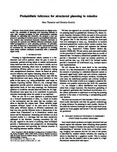
![[PDF] Probabilistic Robotics - Google Sites](https://m.moam.info/img/260x300/pdf-probabilistic-robotics-google-sites_6477d649097c4744708c2820.jpg)


![[PDF] Probabilistic Robotics - Google Sites](https://m.moam.info/img/260x300/pdf-probabilistic-robotics-google-sites_64775e24097c474e708b9fc3.jpg)