Probabilistic Approximations of Signaling Pathway Dynamics

Probabilistic Approximations of Signaling Pathway Dynamics Bing Liu1 , P.S. Thiagarajan1,2 and David Hsu1,2 1

2

NUS Graduate School for Integrative Sciences and Engineering, National University of Singapore Department of Computer Science, National University of Singapore {liubing, dyhsu, thiagu}@comp.nus.edu.sg

Abstract. Systems of ordinary differential equations (ODEs) are often used to model the dynamics of complex biological pathways. We construct a discrete state model as a probabilistic approximation of the ODE dynamics by discretizing the value space and the time domain. We then sample a representative set of trajectories and exploit the discretization and the structure of the signaling pathway to encode these trajectories compactly as a dynamic Bayesian network. As a result, many interesting pathway properties can be analyzed efficiently through standard Bayesian inference techniques. We have tested our method on a model of EGF-NGF signaling pathway [1] and the results are very promising in terms of both accuracy and efficiency.

1

Introduction

Quantitative mathematical models are needed to understand the functioning of complex biological systems. In particular they are needed to capture the dynamics of various intra (and inter)-cellular processes. Here we focus on signaling pathways which typically sense extra-cellular or internal signals and in response, activate a cascade of intra-cellular reactions. A multitude of signaling pathways govern and coordinate the behavior of cells. As might be expected, many disease processes arise from defects in signaling pathways. Thus the study of signaling pathways via quantitative dynamic models is of critical importance. A standard formalism used to model signaling pathways (and other biopathways) is a system of Ordinary Differential Equations (ODEs); the equations describe specific bio-chemical reactions while the variables typically represent concentration levels of molecular species (genes, RNAs, proteins). This formalism can be extended to include discrete aspects [2] and the techniques we develop here can be adapted to such extensions as well. Signaling pathways usually involve a large number of molecular species and bio-chemical reactions. Hence the corresponding ODEs system will not admit closed form solutions. Instead, one will have to resort to numerically generated trajectories to study the dynamics. A second barrier is that the values of many of the parameters (rate constants) associated with the ODEs will be unknown. Even assuming all the parameters are known, the observables of the system will

2

Liu et al.

have very limited precision. Specifically, the initial concentration levels of the various proteins and rate constants will often be available only as intervals of values. Further, experimental data in the form of the measured concentration levels of a few proteins at a small number of time points will also be available only in terms of intervals of values. In addition, the data will often be gathered using a population of cells. Consequently, when numerically simulating the ODEs model, one must resort to Monte Carlo methods to ensure that sufficiently many point values from the relevant intervals of values are being sampled. As a result, analysis tasks such as model validation, parameter estimation and sensitivity analysis will require the generation of a large number of trajectories. This motivates our goal of probabilistically approximating the dynamics of ODEs via discretizations. We start with a system of ODEs and a prior distribution of the initial states. Usually, this prior will consist of a uniform distribution over certain intervals of values of the variables and the rate constants. We then fix a suitable discretization of the value and time domains. This is followed by sampling the prior distribution of initial states to numerically pre-compute and store a representative subset of trajectories induced by the ODEs dynamics. The key idea is to exploit the dependencies/independecies in the pathway structure and the discretization, to compactly encode these trajectories as a time-variant dynamic Bayesian network [3]. The resulting approximation is called the Bayesian Dynamics Model (BDM). Since the trajectories are grouped together through the discretization, our method bridges the mismatch between the accuracy of the results obtained by ODE simulation and the limited precision of experimental data used for model construction and verification. Secondly, the BDM represents the global pathway dynamics more explicitly in the graph structure of the underlying dynamic Bayesian network (DBN). As a result, many interesting pathway properties can be analyzed efficiently through standard Bayesian inference techniques, instead of resorting to a large number of ODE simulations. There is a one-time computational cost incurred to construct the BDM but this cost can be amortized by performing multiple analysis tasks such as expected profiles estimation, parameter estimation, sensitivity analysis etc. using the BDM. We have tested our method on a model of EGF-NGF signaling pathway [1] and the results obtained are very promising in terms of both accuracy and efficiency. In terms of related work, a variety of qualitative and quantitative computational models have been proposed in the recent years to study bio-pathways [2, 4– 6]. Among the quantitative models, one usually distinguishes between populationbased models driven by stochastic simulations and ODEs based models driven by -deterministic- numerical simulations. Clearly, both approaches are needed to cover different contexts. Indeed, our work is, in spirit, related to the discretized approximations presented in [7–9] that can be applied to high level modeling formalism such as PEPA and PRISM. In these cited works, the dynamics of a process-algebra-based description of the bio-pathway is given in terms of a Continuous Time Markov Chain (CTMC) which is then discretized (using the notion of levels) to ease analysis. Apart from the fact that our starting point is

Probabilistic Approximations of Signaling Pathway Dynamics

3

a system of ODEs, a crucial additional step we take is to exploit the structure of the pathway to encode the dynamics more compactly as a dynamic Bayesian network and perform analysis tasks directly on this representation. In a similar vein, we feel that our model is a more compact discrete state model than than the graphical model of a network of non-homogenous Markov processes studied in [10]. We also believe that the techniques proposed in [11], as well as the verification techniques reported in [12, 13] can be adapted to our setting. Interestingly, there have been recent attempts to synthesize ODEs from PEPA model [14], the motivation being that numerical simulations are faster than stochastic simulations. We note however, in our setting, though BDM is a probabilistic graphical model, we do not have to resort to stochastic simulations. The inferencing algorithm we use (the so called Factored Frontier Algorithm [15]), in one sweep, gathers information about the statistical properties of the family of trajectories encoded by the BDM. In the next section, we describe our method for constructing our BDM approximation. In section 3, we present a basic inferencing technique and methods for performing tasks such as parameter estimation and global sensitivity analysis using the BDM. We also simultaneously use a realistic signaling pathway model to evaluate these techniques. In the final section, we summarize the paper and discuss future work. The interested reader can find additional technical material in the form an appendix and relevant supplementary material at [16].

2

The Bayesian Dynamics Model

Conceptually, our approximation technique consists of three steps: 1. We start with a system of ODEs; a discretization of the value space of each variable and rate constant into a finite set of intervals; and a digitalization of the temporal domain of interest into a finite set of time points {t0 , t1 , . . . , tmax }. We also assume a prior distribution of the initial values (usually, a uniform distribution) over some of the intervals of the value space. These initial values will define an uncountably infinite family of trajectories T RAJideal , which in turn, via the discretization, will induce a Markov chain MC ideal . 2. It is impossible to compute MC ideal explicitly. However, it can be approximated by sampling the set of initial values according to the prior and using numerical integration to generate a representative subset T RAJapprox ⊆ T RAJideal of trajectories. Then, using the discretization and simple counting, we can construct the Markov Chain MC approx which will be an approximation of MC ideal . 3. However, MC approx can be very large since the number of states that this Markov chain will be, in the worst case, exponential in the number of variables. To get around this, we exploit the pathway structure (i.e. the way the variables are coupled to each other in the system of ODEs) to represent MC approx compactly as time-variant dynamic Bayesian network. This representation of MC approx is called the Bayesian Dynamics Model (BDM).

4

Liu et al.

We emphasize that this three step procedure is just a conceptual framework; we construct the BDM directly from the given system of ODEs. In what follows, we describe the main technical ideas. The interested reader can find background material and additional details in the appendix portion of the supplementary material. 2.1

ODEs and Flows

We assume a set of ODEs x˙i (t) = fi (x(t), p) involving the continuous realvalued variables {x1 , x2 , . . . , xn } and real-valued parameters {p1 , p2 , . . . , pm }. In our setting, we will often be interested in studying the dynamics for different combinations of values for the parameters. Hence it will be convenient to treat them also as variables. However they will be time-invariant in the sense once their values are fixed at t = 0, these values will not change through the passage of time. Consequently, we will implicitly assume the given system of ODEs to be augmented with m additional differential equations of the form p˙j (t) = 0 with j ranging over {1, 2, . . . , m}. In what follows, we will often let x, v range over IRn+ , the values space of the variables and k range over IRm + , the values space of n+m , the combined values space. the parameters and z range over IR+ In vector form, our system of ODEs may be then represented as Z0 = F (Z). The ODEs will be mainly modeling mass action kinetics or variants such as to be a C 1 → IRn+m Michaelis-Menten kinetics. Hence we can assume F : IRn+m + + (continuously differentiable) function. Furthermore, the variables representing the concentration level of a species within a single cell as well as the parameters capturing the reaction rates will take values from a bounded interval. Hence the domain of F can be restricted to a bounded region D of IRn+m . + Given z0 = (v0 , k) where v0 specifies the initial values of the variables and k specifies the parameters values, the system of ODEs will have a unique solution (due to F ∈ C 1 ) [17]. We shall denote this solution by Z(t) with Z(0) = z0 and Z0 (t) = F (Z(t)). It will be convenient to define the flow Φ : IR+ × D → D of Z0 = F (Z) for arbitrary initial vectors z. It will be a C 0 (continuous) function given by: d (Φ(t, z)) = F (Φ(t, z)) for all t. Φ(t, z) = Z(t) with Φ(0, z) = Z(0) = z and dt 2.2

The Markov Chain MC ideal

Pathways models are usually validated by experimental data available only for a few time points with the concentrations measured at the last time point typically signifying the steady state value. Hence we assume the dynamics is of interest only for discrete time points and that too only up to a maximal time point. Consequently, we fix a time step ∆t > 0 and the time points of interest is ˆ where dˆ · ∆t is assumed to be the set {d · ∆t} with d ranging over {0, 1, . . . , d} the maximal time point of interest. Next we assume that the values of the variables can be observed with only finite precision and accordingly partition the range of each xi into Li intervals [vimin , vi1 ), [vi1 , vi2 ), . . . , [viLi −1 , vimax ]. We denote this set of intervals as Ii . We also

Probabilistic Approximations of Signaling Pathway Dynamics

5

similarly discretize the range of each parameter pj into a set of intervals denoted as In+j . The set I = {Ii }1≤i≤n ∪ {In+j }1≤j≤m is called the discretization. As pointed out earlier, the initial values vector as well as the rate constants (even when they are known) will be given not as point values but as distributions (usually uniform) over the intervals defined by the discretization. We correspondingly assume we are given a prior distribution in the form of a probability density function Υ 0 capturing the distribution of initial values. For example, suppose we are given that the initial values are uniformly distributed within a hypercube Iˆ1 × Iˆ2 × . . . × Iˆn+m , where Iˆi ∈ Ii for each i. Let Iˆi = [li , ui ) and w ˆ i = ui − li . Then the corresponding prior probability density function Υ 0 will be given by: ( 1 if z ∈ Iˆ1 × Iˆ2 × . . . × Iˆn+m , 0 Υ (z) = wˆ1 ·wˆ2 ·...·wˆn+m 0 otherwise. The associated probability space we have in mind is (D, BD , P 0 ) where BD is the Borel σ-algebra over D; the minimal σ-algebra containing the open sets of D under the usual topology. P 0 is the probability distribution induced by Υ 0 and is given by: R P 0 (B) = B Υ 0 (z)dz, for every B ∈ BD . Further, T RAJideal = {Z(t)}t≥0 with Z(0) ∈ Iˆ1 × Iˆ2 × . . . × Iˆn+m is the family of trajectories starting from all the possible points in this hypercube. Since the flow is continuous and hence measurable we can associate a probability 0 0 distribution P t over BD for every t. To define this, let Φ−1 t (B) = {z | Φ(t, z ) ∈ −1 B} for B ∈ BD . Since Φ(t, ·) is measurable, we have Φt (B) ∈ BD too. We can now define P t as: P t (B) = P 0 (Φ−1 t (B)), for every B ∈ BD . Let v be in the range of xi . We define [v] as the interval in which v falls. In other words, [v] = I iff v ∈ I. Similarly, [k] = J if k ∈ J for a parameter value k of pj with J ∈ In+j . Lifting this notation to the vector setting, if z = (v1 , v2 , . . . , vn , k1 , k2 , . . . , km ) ∈ IRn+m , we define [z] = ([v1 ], [v2 ], . . . , [vn ], [k1 ], . . . , [km ]) and refer to it as a + discrete state. An MC-state is a pair (s, d), where s is a discrete state and ˆ d ∈ {1, 2, . . . , d}. We next define P r(s, d) = P d·∆t ({z | z ∈ I1 × I2 × . . . × In+m }), where s = (I1 , I2 , . . . , In+m ). We term the MC-state M to be feasible iff P r(M ) > 0. The transition relation denoted as →, between MC-states is defined via: M = (s, d) → M 0 = (s0 , d0 ) iff d0 = d + 1 and both M and M 0 are feasible and there exist z0 , z, and z0 such that Φ(d · ∆t, z0 ) = z and Φ((d + 1) · ∆t, z0 ) = z0 . Furthermore, [z] = s and [z0 ] = s0 . Let E, F denote, respectively, the event that the system is in the discrete state s at time d · ∆t and in the discrete state s0 at time (d + 1) · ∆t for two feasible MC-states (s, d · ∆t) and (s0 , (d + 1) · ∆t). Let EF = E ∩ F denote joint event {z0 | Φ(d · ∆t, z0 ) ∈ s, Φ((d + 1) · ∆t, z0 ) ∈ s0 }. Consequently, we define the

6

Liu et al.

transition probability P r((s, d) → (s0 , d0 )) = P r(F |E) = P r(EF )/P r(E). Since P r(E) > 0 this transition probability is well-defined. Let M = {M1 , M2 , . . . , Mnˆ } be the set of M-states. We can now define the Markov chain MC ideal = (M, {pij }) with transition probabilities pij = P r(Mi → Mj ) as above. 2.3

The Markov Chain MC approx

MC ideal can not be explicitly computed. Hence we sample z0 a sufficiently larger number of times, say N , according to the prior distribution P 0 (we say more about N below). For each sampled initial z0 , we determine through numerical ˆ We also integration the M-states [Φ(d·∆t, z0 )], with d ranging over {0, 1, . . . , d}. determine the transitions along this trajectory. Then through a simple counting process involving these N trajectories, we compute a Markov chain that we refer to as the MC approx . Since N is finite, there will be an error between the transition probabilities (also the MC-state probabilities) computed using MC approx and the ones defined by MC ideal . By the central limit theorem [18], this error can be probabilistically bounded. In other words, given an error bound  and a confidence level c, we can compute N , the number of samples required to get an error less than or equal to  with likelihood c (the Appendix gives more details). Further, this error will tend to 0 with probability 1 as N tends to ∞. There will be an additional error induced by the pth-order numerical integration method we use to compute the N trajectories. This error will tend to 0 as ∆t tends to 0 or p tends to ∞. However, the number of states of this Markov chain will be exponential in n and hence for many signaling pathways MC approx will be too large a structure. Hence we shall construct a time-variant DBN called the BDM to compactly represent MC approx . We shall however compute the BDM directly from the N sampled trajectories. 2.4

The BDM Representation

In what follows, we assume the basic background concerning Bayesian networks and dynamic Bayesian networks [3]. The graphical structure of the DBN used for our approximation can be derived from the differential equations. It will have n+ m random variables (corresponding to the variables and the parameters) as nodes ˆ For convenience, we for each time slice d · ∆t with d ranging over {0, 1, . . . , d}. will use the same name to denote a variable (parameter) and the corresponding random variable. From the context it should be clear which role is intended. The random variable xi (pj ) can assume as values, the finite set of intervals Ii (In+j ). The variable (parameter) xi (pj ) in the time slice d · ∆t will be written as xdi d (pj ). Edges connecting a node in the d-th slice to a node in the (d+1)-th slice will be determined by the dependencies of the variables and the parameters in the ODEs. Suppose zld is a (variable or parameter) node in the d-th time slice and

Probabilistic Approximations of Signaling Pathway Dynamics

7

zqd+1 is a node in the next time slice. Then there will be an edge from zld to zqd+1 iff zl = zq or zq is a variable node and zl appears in the expression for z˙q in the system of ODEs. As usual, the parents of the node zqd+1 will be the set of nodes of the form zld from which there is an edge into zqd+1 . Suppose, parents(xd+1 )= i d d {z1 , . . . , zl }. Then conditional probability table (CPT) associated with the node xd+1 will have entries of the form P r(xd+1 = I | z1d = I 1 , . . . , zld = I l ) = h with i i k I ranging over Ii and I ranging over Ik and h ∈ [0, 1].

k1

k

3 S + E ES − − → E+P k2

dS dt dE dt dES dt dP dt

0

= −k1 · S · E + k · ES = −k1 · S · E + (k2 + k3 ) · ES = k1 · S · E − (k2 + k3 ) · ES = k3 · ES

Fig. 1. The ODE model of the enzyme-kinetic system and its BDM.

For instance, Figure 1 shows two adjacent slices of a enzyme-kinetic system. In this BDM, the parent nodes of P d+1 are P d , ES d and k3d . As mentioned earlier, the parameters are assumed to not change their values during a run and hence we denote kid as simply ki and there will be no CPTs associated with these nodes. As illustrated by the example, the connectivity between the nodes in successive slices will remain invariant. However, due to the fact that the CPTs associated with the nodes capture the transition probabilities of MC-states, they will be time variant. ˆ n ) states and O((dˆ − 1)K 2n ) MC approx will have, in the worst case, O(dK transitions, where K is the maximum of |Ii | with 1 ≤ i ≤ n + m. In contrast, the ˆ + m)) and the conditional number of nodes in the BDM representation is O(d(n probability table associated each node will have at most O(K R+1 ) entries, where R is the maximal number of parents a node can have. Usually, the reactants in pathway models will be sparsely coupled to each other and hence R will be much smaller than n. For instance, in the case study to be presented, n = 32 and R = 5. Even in cases where R is large, due to the nature of the ODEs we deal with, we can often break up the corresponding node into nodes with smaller fan-in degrees and thus reduce R [16]. To fill up the entries of the CPTs associated with the nodes we randomly choose N combinations of initial values for the variables and the parameters from their prior distribution as before. (If we want a coverage of J samples per interval in an n + m dimensional vector of intervals, then by exploiting the network structure, we can make do with N = JK R+1 samples.) We then perform numerical integration to generate N trajectories and discretize those trajectories by the predefined intervals and compute the conditional probabilities

8

Liu et al.

for each node by simple counting. For example, suppose α trajectories hit (P d = I 0 , ES d = I 00 , k3 = I 000 ) and β of them in turn hit (P d+1 = I), then P r(P d+1 = β I|P d = I 0 , ES d = I 00 , k3 = I 000 ) = α . Further, the MC approx can be easily recovered from this DBN [19]. In this sense, our BDM representation is a principled probabilistic approximation of the dynamics induced by the system of ODEs. Various optimizations can be developed to reduce the practical complexity of the BDM construction. The details can be found in [16]. Though the construction of the BDM involves significant computational effort, it is a one time cost. Moreover, a substantial portion of the computation can be executed in parallel. Further, once the BDM has been constructed, many of the analysis tasks can be performed very efficiently and the one time cost of constructing the BDM can be easily amortized. We present some experimental results in support of this in the next section.

3

Analysis

We now present some of the analysis techniques that we have developed so far for the BDM representation. These techniques are based on the basic Bayesian inference method called the F F (Factored Frontier) algorithm [15] and can be used to answer elementary probabilistic queries as well for performing parameter (rate constants) estimation and sensitivity analysis. Our goal here is not to develop new algorithms to solve these problems. Rather, we wish to demonstrate how standard techniques for tackling these problems can be adapted to BDM framework in a straightforward manner. We validate our techniques using a relatively large signaling pathway and show the relevant experimental results along with our techniques. 3.1

The EGF-NGF signaling pathway and its BDM

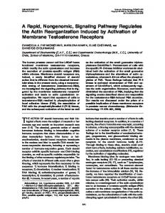
PC12 cells are a valuable model system in neuroscience. They proliferate in response to EGF stimulation but differentiate into sympathetic neurons in response to NGF. This interesting phenomenon has been intensively studied [20]. It has been reported that the signal specificity is correlated with different Erk dynamics. Specifically, a transient activation of Erk1/2 has been associated with cell proliferation, while a sustained activity has been linked to differentiation. How EGF and NGF affect the dynamics of active Erk through a network of intermediate signaling proteins is shown schematically in Figure 2. This model not only includes a common pathway to Erk through Ras shared by both the EGFR and NGFR, but also includes two important side branches through PI3K and C3G, which introduce multiple feedback loops thus complicating the dynamics. The ODE model of this pathway is available in the BioModels database3 . It consists of 32 differential equations and 48 associated rate parameters (estimated from multiple sets of experimental data). 3

http://www.ebi.ac.uk/biomodels/

Probabilistic Approximations of Signaling Pathway Dynamics

9

... ... d[f reeEGF R ] = 0 .0121008× [boundEGF R ] dt 0 .0000218503×[ EGF ] × [ f reeEGF R ] d[boundEGF R ] = 0 .0000218503× [ EGF ] × [ f reeEGF R ] dt 0.0121008 × [boundEGF R ] d[Sos] 1611.97× [P90Rsk* ] × [Sos] = dt [Sos] + 896896 694.731× [boundEGF R ] × [Sos] [Sos] + 6086070 389.428 × [boundN GF R ] × [Sos] [Sos] + 211.266 d[Sos*] 694.731× [boundEGF R ] × [Sos] = dt [Sos] + 6086070 389.428× [boundN GF R ] × [Sos] + [Sos] + 211.266 1611.97× [P90Rsk* ] × [Sos] [Sos] + 896896 ... ...

Fig. 2. EGF-NGF pathway [1]

To construct the BDM, we first derived its graph from its ODEs. We then discretized the ranges of each variable and parameter into 5 equal-size intervals and fixed the time step ∆t to be 1 minute. Our experimental data (western blot) is such that 5 uniform intervals seems an appropriate choice. However our construction can be easily extended to non-uniform values intervals and time points. To fill up the conditional probability tables associated with the nodes, 3 × 106 trajectories were generated up to 100 mins by sampling initial states and parameters from the prior which are assumed to be uniform distributions over certain intervals (see [16]). The computational workload was distributed on 10 Opteron 2.2GHz processors in a cluster. It took around 4 hours to construct the BDM. All the subsequent experiments reported below were done using an Intel Xeon 2.8GHz processor.

3.2

Probabilistic Inference

As pointed out earlier, although the dynamics defined by the ODEs is deterministic, to answer a basic query such as “what will be the concentration of the protein xi at time t? ” one will have to numerically generate a representative sample of trajectories and compute the average of the values for xi at t yielded by the individual trajectories. Using our BDM approximation, we can answer such a basic query and other more sophisticated queries by Bayesian inference. Specifically, given a Bayesian network, some observed evidence and some knowledge about the distribution of values of a set of variables, Bayesian inference aims to compute posterior distribution for a set of query variables. In our setting, the observed evidence refers to the initial conditions, known parameters, and experimental data. Query variables potentially refer to all the random variables in the BDM. We adopt the approximate algorithm known as the Factored Frontier (FF) algorithm [15]. It approximates joint distributions over each time point as a product of marginal

10

Liu et al. 1 .2 0 x 1 0

4

9 .6 0 x 1 0

3

7 .2 0 x 1 0

3

4 .8 0 x 1 0

3

2 .4 0 x 1 0

3

b o u n d N G F R

0 .0 0

1 .3 0 x 1 0

5

1 .0 4 x 1 0

5

7 .8 0 x 1 0

4

5 .2 0 x 1 0

4

2 .6 0 x 1 0

4

S o s *

0 .0 0 0

2 0

4 0

6 0

8 0

5

7 .8 0 x 1 0

4

5 .2 0 x 1 0

4

2 .6 0 x 1 0

4

p 9 0 R S K *

0

2 0

4 0

6 0

8 0

5 .2 0 x 1 0

4

4

2 .6 0 x 1 0

4

2 .6 4 0 x 1 0

4

4

5 .2 8 0 x 1 0

5

4

7 .8 0 x 1 0

7 .9 2 0 x 1 0

5

5

1 .0 4 x 1 0

5

1 .0 5 6 x 1 0

1 .3 0 x 1 0 1 .3 2 0 x 1 0

C 3 G *

0

2 0

4 0

6 0

8 0

R a s *

0 .0 0

0 .0 0 0

1 0 0

0

1 0 0

5

6 .6 0 0 x 1 0

6 .6 0 0 x 1 0

5

1 .0 4 x 1 0

0 .0 0

1 0 0

5

1 .3 0 x 1 0

2 0

4 0

6 0

8 0

0

1 0 0

1 2 0 0 0 0

1 .3 2 0 x 1 0

5

9 6 0 0 0

1 .0 5 6 x 1 0

5

7 2 0 0 0

7 .9 2 0 x 1 0

4

5 .2 8 0 x 1 0

4

2 .6 4 0 x 1 0

4

2 0

4 0

6 0

8 0

1 0 0

1 3 2 0 0 0

5 .2 8 0 x 1 0

5

3 .9 6 0 x 1 0

5

2 .6 4 0 x 1 0

5

1 .3 2 0 x 1 0

5

5 .2 8 0 x 1 0

5

3 .9 6 0 x 1 0

5

E rk *

M e k *

1 0 5 6 0 0

P I3 K *

7 9 2 0 0

4 8 0 0 0

5 2 8 0 0

1 .3 2 0 x 1 0

5

0

2 0

4 0

6 0

8 0

1 0 0

2 4 0 0 0

2 6 4 0 0

0 .0 0 0

0 .0 0 0

A K T *

5

2 .6 4 0 x 1 0

0

2 0

4 0

6 0

8 0

1 0 0

0 .0 0 0

0

0 0

2 0

4 0

6 0

8 0

1 0 0

R a p 1

0

2 0

4 0

6 0

8 0

1 0 0

0

2 0

4 0

6 0

8 0

1 0 0

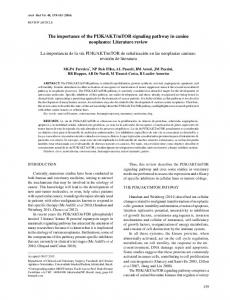
Fig. 3. Simulation results of EGF-NGF signaling pathway. Solid lines represent nominal profiles and dash lines represent BDM simulation profiles.

distributions and computes the posterior distribution according to: P r(xdi |D) =

X I

(P r(xdi |P a(xdi ) = I)

Y

P r(u|D)).

(1)

u∈P a(xd i)

Here P r(u|D) are the marginal distributions over the parents, D is the evidence, and P a(xi ) denotes the parents of xi . The implementation of FF is straightforward. By storing P r(xdi |P a(xdi )) in the conditional probability tables and propagating P r(u|D) to the next time point, we can use equation 1 to compute ˆ + m)K R+1 ), where K P r(xdi |D). The time complexity of this algorithm is O(d(n is the maximal number of intervals associated with a variable or rate constant’s value domain. Further, R is the maximal number of parents a node can have. Using this algorithm, and with some additional simple computations, many queries can be answered. For instance, we identify each interval I = [l, u) in I with its mid-point l+u 2 . Then after inferring the probability distribution of xi over intervals, the expected value E(xdi ) at a time slice d can be computed and used to validate the model by comparing it with the cell population based data that may be available for xi at d · ∆t. To test the quality of our approximation, we implemented Monte Carlo integration for the ODE model to get good estimates by sampling. Specifically, we numerically generated a number of random trajectories -according to the priorusing ODEs, discretized them and computed the average values of the variables at the chosen time points. Our experiments show that the average values converge when the number of random trajectories generated is roughly 104 . The averaged trajectories projected to individual protein concentration time series values are termed to be the nominal simulation profiles. Using the implemented FF algorithm, the mean of each variable over time was computed. The resulting time profiles are termed to be the BDM-simulation profiles. As summarized in Figure 3, our BDM-simulation profiles fit the nominal simulation profiles quite well for most of the cases. In terms of running time, a single execution of FF inference requires 0.29 seconds while generating a stable nominal profile requires 386.4 seconds. Thus, the total computation time will be sharply reduced by our approach when many

Probabilistic Approximations of Signaling Pathway Dynamics

11

such “queries” need to be answered. In the next subsection, we will further demonstrate this advantage by carrying out a simulation-intensive analysis task. 3.3

Parameter estimation.

Lack of knowledge about the parameters and hence the need to perform parameter estimation using limited data has long been identified as a major bottleneck of pathway modeling. Current approaches to parameter estimation formulate it as a non-linear optimization problem [21]. A typical procedure will involve searching in a high dimensional solution space, in which each point represents a vector of parameter values. Whether a point is good or not is measured by the objective function, which will capture the difference between experimental data and prediction generated by simulations using the corresponding parameters. For a large pathway model, one often needs to evaluate a very large number of solution points involving a numerical integration for each evaluation. This makes the whole process computationally intensive. The BDM representation allows us to carry out the search for good parameter values in a hierarchical manner. Due to the discretized nature of the BDM, the solution space is transformed to a rectilinear grid consisting of a space-filling tessellation by hyperrectangles that we call blocks. An important observation is that kinetic parameters are often robust [22]. In other words, the points around the best solution in the search space will also have relatively small objective values. Thus, instead of searching point by point in the solution space, we can first search for a few promising blocks and then take a closer look within these small blocks. Therefore, the general scheme of our “grid search” algorithm will consist of two phases: (1) identify good blocks, (2) do local search within candidate blocks. We note that phase(2) is necessary only when we aim to estimate parameters with finer granularity than the granularity of the BDM’s discretization. Otherwise, one can skip phase(2) and return a probabilistic estimate (typically a Maximal Likelihood Estimate) of a combination of intervals of parameter values. For executing phase(1), we can apply any standard search algorithms over the discretized search space. As the discretized search space is much smaller than the original one, simple direct search algorithm such as Hooke & Jeeves’s search [23] can be adopted and the overall search process will only require a small number of executions of the FF algorithm. In order to test the performance of the BDM-based parameter estimation method, we synthesized experimental time series data for 9 (out of 32) proteins {bounded EGFR, bounded NGFR, active Sos, active C3G, active Akt, active p90RSK, active Erk, active Mek, active PI3K}, measured at the time points {2, 5, 10, 20, 30, 40, 50, 60, 80, 100} (min).This data was synthesized using prior knowledge about initial conditions and parameters [16]. To mimic western blot data which is cell population based, we first averaged 104 random trajectories generated by sampling initial states and rate constants, and then added observation noise with variance 5% to the simulated values. With the assumed measurement precision, those values were discretized into 5 intervals, which represent the concentration levels in western blot data. We reserved the data of 7

12

Liu et al. 1 .2 0 x 1 0

4

9 .6 0 x 1 0

3

b N G F R

5

7 .8 0 x 1 0

4

5 .2 0 x 1 0

4

2 .6 0 x 1 0

4

1 .3 0 x 1 0

5

6 .6 0 0 x 1 0

5

1 .0 4 x 1 0

5

5 .2 8 0 x 1 0

5

7 .8 0 x 1 0

4

3 .9 6 0 x 1 0

5

5 .2 0 x 1 0

4

2 .6 4 0 x 1 0

5

2 .6 0 x 1 0

4

1 .3 2 0 x 1 0

5

M e k *

A K T *

C 3 G *

3

4 .8 0 x 1 0

3

0 .0 0

0 .0 0

0

2 0

4 0

6 0

8 0

0 .0 0 0

1 0 0 0

2 0

4 0

6 0

8 0

1 0 0

0

5 .2 8 0 x 1 0

5

4

7 .8 0 x 1 0

4

3 .9 6 0 x 1 0

5

4

5 .2 0 x 1 0

4

2 .6 4 0 x 1 0

5

5 .2 0 x 1 0

6 .6 0 0 x 1 0

5

7 .8 0 x 1 0

5

1 .0 4 x 1 0

5

1 .3 0 x 1 0

5

1 .0 4 x 1 0

5

1 .3 0 x 1 0

2 .6 0 x 1 0

5

1 .0 4 x 1 0

3

7 .2 0 x 1 0

2 .4 0 x 1 0

1 .3 0 x 1 0

S o s *

4

2 .6 0 x 1 0

0

2 0

4 0

6 0

8 0

1 0 0

4 0

6 0

8 0

4

1 .3 2 0 x 1 0

0

1 0 0

E rk *

p 9 0 R S K *

0

2 0

4 0

6 0

8 0

1 0 0

1 .3 0 x 1 0

5

1 .0 4 x 1 0

5

7 .8 0 x 1 0

4

5 .2 0 x 1 0

4

2 .6 0 x 1 0

4

2 0

4 0

6 0

8 0

1 0 0

P I3 K *

5

0 .0 0

0 .0 0 0

0 .0 0

0 .0 0

2 0

0

2 0

4 0

6 0

8 0

0

1 0 0

2 0

4 0

6 0

8 0

1 0 0

(b )

(a )

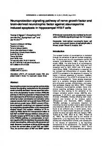
Fig. 4. Parameter estimation results. (a) BDM-simulation profiles vs. training data. (b) BDM-simulation profiles vs. test data.

proteins for training the parameters and reserved the rest data for testing the quality of the estimated parameter values. Assuming that 20 of the 48 parameter values are unknown, a modified version of Hooke & Jeeves algorithm was implemented to search for in the discretized parameter space. The parameters obtained can be found in [16]. As shown in Figure 4, the BDM-simulation profiles generated using the estimated parameters obtained (with the match to training data as shown) has good agreement with the test data. We compared the efficiency and quality of our results with the following ODEs based optimization algorithms: Levenberg-Marquardt (LM), Genetic Algorithm (GA), Stochastic Ranking Evolutionary Strategy (SRES), and Particle Swarm Optimization (PSO). These optimization algorithms were executed using the COPASI [24] tool. We scored the resulting parameters obtained from all the algorithms using the weighted sum-of-squares difference between the experimental data and the corresponding simulation profiles (i.e. low scores correspond to low errors). The results are summarized in Figure 5, which suggests that our method achieves a good balance between accuracy and performance. We also note that the cost of constructing the BDM representation gets rapidly amortized. In fact the savings become even more significant when we perform additional analysis tasks such as sensitivity analysis. 1 .8 5 E + 0 1 0

4 0 0 0

1 .3 9 E + 0 1 0

3 0 0 0

2 .7 8 E + 0 0 9

6 0 0

1 .8 5 E + 0 0 9

4 0 0

9 .2 6 E + 0 0 8

2 0 0

0 .0 0 E + 0 0 0

T im e [s ]

E rro r

E rro r T im e

0

L M

G A

S R E S

P S O

B D M

Fig. 5. Performance comparison of our parameter estimation method (BDM) and 4 other methods.

Probabilistic Approximations of Signaling Pathway Dynamics

3.4

13

Global sensitivity analysis.

Sensitivity analysis has been used to identify the critical parameters in signal transduction. To overcome the limitations of traditional local sensitivity analysis methods global methods have been proposed recently, e.g. multi-parametric sensitivity analysis (MPSA) [25]. The MPSA procedure consists of: (1) draw samples from parameter space and for each combination of parameters, compute the weighted sum of squared error between experimental data and predictions generated by selected parameters; (2) classify the sampled parameter sets into two classes (good and bad) using a threshold error value; (3) plot the cumulative frequency of the parameter values associated with the two classes; (4) evaluate the sensitivities as the Kolmogorov-Smirnov statistic of cumulative frequency curves. To improve this process, [25] adopts Latin hypercube sampling (LHS) since it requires fewer samples while guaranteeing that individual parameter ranges are evenly covered. In our BDM setting, MPSA can be done in a similar manner using LHS since the parameter space is discretized into blocks. In addition, the number of samples used to reach convergence is reduced since we can quickly evaluate the whole block instead of having to draw samples from a block. We modified and implemented the MPSA method for the BDM. Using the same experimental data set introduced in previous subsection, the global sensitivities (K-S statistics) of the parameters were computed. The results are shown in Figure 6. The cumulative frequency distributions for the acceptable and unacceptable cases of the rate constants can be found in [16]. Specifically, the reactions involved in the phosphorylation of Erk (k23 ), Mek (k17 ), Akt (k34 ) and p90RSK (k28 ) have the highest sensitivities, indicating that these reactions affect the system behavior most directly. These results are consistent with previous findings [20]. 0 .2 5

S e n s itiv ity

0 .2 0

0 .1 5

0 .1 0

0 .0 5

0 .0 0

k 1

k 2

k 3

k 4

k 1 1

k 1 2

k 1 5

k 1 7

k 2 3

k 2 7

k 2 8

k 2 9

k 3 3

k 3 4

k 3 7

k 3 8

k 3 9

k 4 0

k 4 3

k 4 4

Fig. 6. Parameter sensitivities

The MPSA method adopts Monte Carlo strategy for the ODE model. We recorded the running time of the algorithm till the K-S values converged. The total running time of the ODEs based MPSA method was about 22 hours, while the MPSA method based on the BDM required only 34 minutes.

14

Liu et al.

4

Discussion

We have proposed a probabilistic approximation scheme for signaling pathway dynamics specified as a system of ODEs. Given a discretization and an initial distribution, it consists of pre-computing and storing a representative sample of trajectories induced by the system of ODEs. We use a dynamic Bayesian network representation, called the Bayesian Dynamics Model, to compactly represent these trajectories by exploiting the pathway structure. Basically, the underlying graph of the BDM captures the dependencies of the variables on other variables and rate constants as defined by the system of ODEs. Due to the probabilistic graphical representation, a variety of analysis questions concerning the pathway dynamics traditionally addressed using Monte Carlo simulations can be converted to Bayesian inference and solved more efficiently. Using the FF algorithm for doing basic Bayesian inference, we have adapted standard parameter estimation and sensitivity analysis algorithms to the BDM setting. We have demonstrated the applicability of our techniques with the help of the good sized EGF-NGF signaling pathway. A number of further lines of work suggest themselves. Firstly, we need to apply our method to a variety of pathway models. We are currently doing so in collaboration with biologists. Secondly, it will be useful to augment the ODE model with some discrete features but this should be easy to achieve. A more challenging issue is to abstract the BDM representation to an input-output transducer so that one can efficiently model networks of pathways and inter-cellular interactions models. Finally, it will be important to develop formal verification techniques based on the BDM representation. In this context, it is worth noting that the FF algorithm can compute the marginal probabilities of the discretized values of variables at specific time points. Hence a good starting point will be to develop probabilistic bounded model checking methods for specifications based on the BDM model.

References 1. Brown, K.S., Hill, C.C., Calero, G.A., Lee, K.H., Sethna, J.P., Cerione, R.A.: The statistical mechanics of complex signaling networks: nerve growth factor signaling. Phys. Biol. 1, 184–195 (2004) 2. Matsuno, H., Tanaka, Y., Aoshima, H., Doi, A., Matsui, M., Miyano, S.: Biopathways representation and simulation on hybrid functional Petri net. In Silico Biol. 3(3), 389–404 (2003) 3. Murphy, K.P.: Dynamic Bayesian Networks: Representation, Inference and Learning. PhD thesis, University of California, Berkeley (2002) 4. Antoniotti, M., Policriti, A., Ugel, N., Mishra, B.: XS-systems: extended s-systems and algebraic differential automata for modeling cellular behavior. In Sahni, S., Prasanna, V.K., Shukla, U. (eds.) HiPC 2002. LNCS, vol. 2552, pp. 431–442. Springer, Heidelberg (2002) 5. de Jong, H., Page, M.: Search for steady states of piecewise-linear differential equation models of genetic regulatory networks. IEEE/ACM T. Comput. Bi. 5(2), 208–223 (2008)

Probabilistic Approximations of Signaling Pathway Dynamics

15

6. Ghosh, R., Tomlin, C.: Symbolic reachable set computation of piecewise affine hybrid automata and its application to biological modelling: Delta-notch protein signalling. Systems Biol. 1(1), 170–183 (2004) 7. Calder, M., Gilmore, S., Hillston, J.: Modelling the influence of RKIP on the ERK signalling pathway using the stochastic process algebra PEPA. In Trans. on Comput. Syst. Biol. VII. LNCS, vol. 4230, pp. 1–23. Springer, Heidelberg (2006) 8. Calder, M., Vyshemirsky, V., Gilbert, D., Orton, R.: Analysis of signalling pathways using continuous time Markov chains. In Trans. on Comput. Syst. Biol. VI. LNCS, vol. 4220, pp. 44–67. Springer, Heidelberg (2006) 9. Ciocchetta, F., Degasperi, A., Hillston, J., Calder, M.: CTMC with levels models for biochemical systems. Preprint submitted to Elsevier (2009) 10. Nodelman, U., Shelton, C.R., Koller, D.: Continuous time Bayesian networks. In: Proceedings of the 18th Conference in Uncertainty in Artificial Intelligence, pp. 378–387. Alberta, Canada (2002) 11. Langmead, C., Jha, S., Clarke, E.: Temporal logics as query languages for dynamic Bayesian networks: Application to D. Melanogaster embryo development. Technical report, Carnegie Mellon University (2006) 12. Clarke, E.M., Faeder, J.R., Langmead, C.J., Harris, L.A., Jha, S.K., Legay, A.: Statistical model checking in BioLab: Applications to the automated analysis of T-Cell receptor signaling pathway. In Heiner, M., Uhrmacher, A.M. (eds.) CMSB 2008. LNCS, vol. 5307, pp. 231–250. Springer, Heidelberg (2008) 13. Heath, J., Kwiatkowska, M., Norman, G., Parker, D., Tymchyshyn, O.: Probabilistic model checking of complex biological pathways. Theor. Comput. Sc. 319(3), 239–257 (2008) 14. Geisweiller, N., Hillston, J., Stenico, M.: Relating continuous and discrete PEPA models of signalling pathways. Theor. Comput. Sc. 404(2), 97–111 (2008) 15. Murphy, K.P., Weiss, Y.: The factored frontier algorithm for approximate inference in DBNs. In: Proceedings of the 17th Conference in Uncertainty in Artificial Intelligence, pp. 378–385. San Francisco, CA, USA (2001) 16. Supplementary Materials: http://www.comp.nus.edu.sg/~rpsysbio/cmsb09. 17. Ammann, H.: Ordinary Differential Equations: An Introduction to Nonlinear Analysis. Walter de Gruyter (1990) 18. Durrett, R.: Probability: Theory and Examples. Duxbury Press (2004) 19. Nunez, L.M.: On the relationship between temporal Bayes networks and Markov chains. Master’s thesis, Brown University (1989) 20. Kholodenko, B.N.: Untangling the signalling wires. Nat. Cell Biol. 9(3), 247–249 (2007) 21. Banga, J.R.: Optimization in computational systems biology. BMC Syst. Biol. 2(47), 1–7 (2008) 22. Gutenkunst, R.N., Waterfall, J.J., Casey, F.P., Brown, K.S., Myers, C.R., Sethna, J.P.: Universally sloppy parameter sensitivities in systems biology. PLoS Comput. Biol. 3(10), 1871–1878 (2007) 23. Hooke, R., Jeeves, T.A.: “Direct search” solution of numerical and statistical problems. J. ACM. 8(2), 212–229 (1961) 24. Hoops, S., Sahle, S., Gauges, R., Lee, C., Pahle, J., Simus, N., Singhal, M., Xu, L., Mendes, P., Kummer, U.: COPASI - a COmplex PAthway SImulator. Bioinformatics 22(24), 3067–3074 (2006) 25. Cho, K.H., Shin, S.Y., Kolch, W., Wolkenhauer, O.: Experimental design in systems biology, based on parameter sensitivity analysis using a monte carlo method: A case study for the TNFα-mediated NF-κB signal transduction pathway. Simulation 79(12), 726–739 (2003)