Probabilistic Graphical Model Structure Learning ...

No d’ordre NNT : 2017LYSE1003

THÈSE DE DOCTORAT DE L’UNIVERSITÉ DE LYON opérée au sein de l’Université Claude Bernard Lyon 1 École Doctorale ED512 Infomath Spécialité de doctorat : Informatique

Soutenue publiquement le 13 janvier 2017, par :

Maxime Gasse

Apprentissage de Structure de Modèles Graphiques Probabilistes: Application à la Classification Multi-Label Devant le jury composé de : Céline Robardet, Professeur, INSA Lyon Christophe Gonzales, Professeur, Université Paris 6 Jose M. Peña, Associate Professor, Linköping University Elisa Fromont, Maître de Conférence, Université Jean Monnet Willem Waegeman, Professor, Ghent University Veronique Delcroix, Maître de Conférence, Université de Valenciennes Alexandre Aussem, Professeur, Université Lyon 1 Haytham Elghazel, Maître de Conférence, Polytech Lyon

Présidente Rapporteur Rapporteur Examinatrice Examinateur Examinatrice Directeur de thèse Co-directeur de thèse

UNIVERSITÉ CLAUDE BERNARD - LYON 1 Président de l’Université Président du Conseil Académique Vice-président du Conseil d’Administration Vice-président du Conseil Formation et Vie Universitaire Vice-président de la Commission Recherche Directrice Générale des Services

M. le Professeur Frédéric FLEURY M. le Professeur Hamda BEN HADID M. le Professeur Didier REVEL M. le Professeur Philippe CHEVALIER M. Fabrice VALLÉE Mme Dominique MARCHAND

COMPOSANTES SANTÉ Faculté de Médecine Lyon Est - Claude Bernard Faculté de Médecine et de Maïeutique Lyon Sud - Charles Mérieux Faculté d’Odontologie Institut des Sciences Pharmaceutiques et Biologiques Institut des Sciences et Techniques de la Réadaptation Département de formation et Centre de Recherche en Biologie Humaine

Directeur : M. le Professeur G.RODE Directeur : Mme la Professeure C. BURILLON Directeur : M. le Professeur D. BOURGEOIS Directeur : Mme la Professeure C. VINCIGUERRA Directeur : M. X. PERROT Directeur : Mme la Professeure A-M. SCHOTT

COMPOSANTES ET DÉPARTEMENTS DE SCIENCES ET TECHNOLOGIE Faculté des Sciences et Technologies Département Biologie Département Chimie Biochimie Département GEP Département Informatique Département Mathématiques Département Mécanique Département Physique UFR Sciences et Techniques des Activités Physiques et Sportives Observatoire des Sciences de l’Université de Lyon Polytech Lyon Ecole Supérieure de Chimie Physique Electronique Institut Universitaire de Technologie de Lyon 1 Ecole Supérieure du Professorat et de l’Education Institut de Science Financière et d’Assurances

Directeur : Directeur : Directeur : Directeur : Directeur : Directeur : Directeur : Directeur :

M. F. DE MARCHI M. le Professeur F. THEVENARD Mme C. FELIX M. Hassan HAMMOURI M. le Professeur S. AKKOUCHE M. le Professeur G. TOMANOV M. le Professeur H. BEN HADID M. le Professeur J-C. PLENET

Directeur : M. Y.VANPOULLE Directeur : Directeur : Directeur : Directeur : Directeur : Directeur :

M. B. GUIDERDONI M. le Professeur E.PERRIN M. G. PIGNAULT M. le Professeur C. VITON M. le Professeur A. MOUGNIOTTE M. N. LEBOISNE

Remerciements

En premier lieu, je tiens à exprimer toute ma gratitude aux membres du jury pour l’attention qu’ils ont portée à l’évaluation de mes travaux de thèse. En particulier, je voudrais remercier mes rapporteurs, le Professeur Jose M. Peña et le Professeur Christophe Gonzales, pour le travail considérable qu’ils ont consacré à la lecture assidue de ce long mémoire. J’adresse de chaleureux remerciements envers mes encadrants, le Professeur Alexandre Aussem et le Docteur Haytham Elghazel, pour la confiance qu’ils m’ont accordée. Au delà des échanges scientifiques, ils ont sû me faire profiter de leur expérience précieuse du monde de la recherche, qui m’était jusqu’alors inconnu. Surtout, j’ai pu jouir tout au long de cette thèse d’une grande liberté intellectuelle pour laquelle je suis très reconnaissant. Je remercie l’ensemble des personnels du laboratoire LIRIS et de l’université de Lyon, et en particulier le personnel administratif que j’ai pu côtoyer, Isabelle, Brigitte, Jean-Pierre, Catherine, pour son efficacité et sa bienveillance. Je remercie bien sûr mes collègues de bureau, malheureusement trop nombreux pour être cités ici, pour toutes ces discussions passionnantes le midi ou autour d’un café. Cette atmosphère chaleureuse et amicale, dans un environnement scientifique stimulant, ont largement contribué à mon épanouissement au cours de ces quatre années de recherches. Il convient également de remercier l’union européenne ainsi que l’état français qui ont financé cette thèse, et m’ont permis de vivre décemment de mes activités de recherche durant quatre ans. Je tiens à remercier mes proches, mes amis, ma famille, pour leur soutien ou simplement leur présence. Mener à bien une thèse de doctorat est une expérience passionnante, mais également laborieuse à bien des égards, ainsi on apprécie pouvoir se ressourcer ailleurs lors des passages à vide. Je remercie enfin Charlotte qui m’a supporté toutes ces années, et continue à le faire aujourd’hui.

v

Probabilistic Graphical Model Structure Learning: Application to Multi-Label Classification

Maxime Gasse, Ph.D thesis

Résumé

Dans cette thèse, nous nous intéressons au problème spécifique de l’apprentissage de structure de modèles graphiques probabilistes, c’est-à-dire trouver la structure la plus efficace pour représenter une distribution, à partir seulement d’un ensemble d’échantillons D ∼ p(v). Dans une première partie, nous passons en revue les principaux modèles graphiques probabilistes de la littérature, des plus classiques (modèles dirigés, non-dirigés) aux plus avancés (modèles mixtes, cycliques etc.). Puis nous étudions particulièrement le problème d’apprentissage de structure de modèles dirigés (réseaux Bayésiens), et proposons une nouvelle méthode hybride pour l’apprentissage de structure, H2PC (Hybrid Hybrid Parents and Children), mêlant une approche à base de contraintes (tests statistiques d’indépendance) et une approche à base de score (probabilité postérieure de la structure). Dans un second temps, nous étudions le problème de la classification multi-label, visant à prédire un ensemble de catégories (vecteur binaire y P (0, 1)m ) pour un objet (vecteur x P Rd ). Dans ce contexte, l’utilisation de modèles graphiques probabilistes pour représenter la distribution conditionnelle des catégories prend tout son sens, particulièrement dans le but minimiser une fonction coût complexe. Nous passons en revue les principales approches utilisant un modèle graphique probabiliste pour la classification multi-label (Probabilistic Classifier Chain, Conditional Dependency Network, Bayesian Network Classifier, Conditional Random Field, SumProduct Network), puis nous proposons une approche générique visant à identifier une factorisation de p(y|x) en distributions marginales disjointes, en s’inspirant des méthodes d’apprentissage de structure à base de contraintes. Nous démontrons plusieurs résultats théoriques, notamment l’unicité d’une décomposition minimale, ainsi que trois procédures quadratiques sous diverses hypothèses à propos de la distribution jointe p(x, y). Enfin, nous mettons en pratique ces résultats afin d’améliorer la classification multi-label avec les fonctions coût F-loss et zero-one loss.

ix

Abstract

In this thesis, we address the specific problem of probabilistic graphical model structure learning, that is, finding the most efficient structure to represent a probability distribution, given only a sample set D ∼ p(v). In the first part, we review the main families of probabilistic graphical models from the literature, from the most common (directed, undirected) to the most advanced ones (chained, mixed etc.). Then we study particularly the problem of learning the structure of directed graphs (Bayesian networks), and we propose a new hybrid structure learning method, H2PC (Hybrid Hybrid Parents and Children), which combines a constraint-based approach (statistical independence tests) with a score-based approach (posterior probability of the structure). In the second part, we address the multi-label classification problem, which aims at assigning a set of categories (binary vector y P (0, 1)m ) to a given object (vector x P Rd ). In this context, probabilistic graphical models provide convenient means of encoding p(y|x), particularly for the purpose of minimizing general loss functions. We review the main approaches based on PGMs for multi-label classification (Probabilistic Classifier Chain, Conditional Dependency Network, Bayesian Network Classifier, Conditional Random Field, Sum-Product Network), and propose a generic approach inspired from constraint-based structure learning methods to identify the unique partition of the label set into irreducible label factors (ILFs), that is, the irreducible factorization of p(y|x) into disjoint marginal distributions. We establish several theoretical results to characterize the ILFs based on the compositional graphoid axioms, and obtain three generic procedures under various assumptions about the conditional independence properties of the joint distribution p(x, y). Our conclusions are supported by carefully designed multi-label classification experiments, under the F-loss and the zero-one loss functions.

xi

Contents

Introduction

1

1 Background and notation

3

1.1 Probability theory . . . . . . . . . . . . . . . . . . . . . . . . . . . . .

3

1.1.1 Probability spaces . . . . . . . . . . . . . . . . . . . . . . . . .

3

1.1.2 Random variables

. . . . . . . . . . . . . . . . . . . . . . . .

7

1.1.3 Independence models . . . . . . . . . . . . . . . . . . . . . .

13

1.2 Graph theory . . . . . . . . . . . . . . . . . . . . . . . . . . . . . . .

16

1.2.1 Connectivity, paths, walks, cycles . . . . . . . . . . . . . . . .

16

1.2.2 Classes of graphs . . . . . . . . . . . . . . . . . . . . . . . . .

17

2 Probabilistic graphical models

19

2.1 Classical graphical models . . . . . . . . . . . . . . . . . . . . . . . .

20

2.1.1 Undirected graphs . . . . . . . . . . . . . . . . . . . . . . . .

20

2.1.2 Directed acyclic graphs . . . . . . . . . . . . . . . . . . . . . .

27

2.2 Advanced graphical models . . . . . . . . . . . . . . . . . . . . . . .

41

2.2.1 Bi-directed graphs . . . . . . . . . . . . . . . . . . . . . . . .

42

2.2.2 Chain graphs . . . . . . . . . . . . . . . . . . . . . . . . . . .

43

2.2.3 Mixed graphs . . . . . . . . . . . . . . . . . . . . . . . . . . .

54

2.3 Discussion . . . . . . . . . . . . . . . . . . . . . . . . . . . . . . . . .

62

2.3.1 Trends . . . . . . . . . . . . . . . . . . . . . . . . . . . . . . .

63

2.3.2 Limitations . . . . . . . . . . . . . . . . . . . . . . . . . . . .

65

3 Bayesian network structure learning

71

3.1 Motivation . . . . . . . . . . . . . . . . . . . . . . . . . . . . . . . . .

71

3.2 The score-based approach . . . . . . . . . . . . . . . . . . . . . . . .

73

3.2.1 Bayesian scores . . . . . . . . . . . . . . . . . . . . . . . . . .

74

3.2.2 Information-theoretic scores . . . . . . . . . . . . . . . . . . .

77

3.2.3 The optimization problem . . . . . . . . . . . . . . . . . . . .

81

3.2.4 Meek’s conjecture . . . . . . . . . . . . . . . . . . . . . . . . .

81

3.3 The constraint-based approach . . . . . . . . . . . . . . . . . . . . .

82

3.3.1 Conditional independence tests . . . . . . . . . . . . . . . . .

83

3.3.2 The faithfulness assumption . . . . . . . . . . . . . . . . . . .

84

3.3.3 Algorithms . . . . . . . . . . . . . . . . . . . . . . . . . . . .

84

xiii

3.4 The hybrid approach . . . . . . . . . . . . . . . . . . . . . . . . . . .

90

3.4.1 Early works . . . . . . . . . . . . . . . . . . . . . . . . . . . .

92

3.4.2 Max-Min Hill-Climbing (MMHC) . . . . . . . . . . . . . . . .

92

3.5 Our contribution: a new hybrid algorithm . . . . . . . . . . . . . . .

93

3.5.1 The ideal skeleton . . . . . . . . . . . . . . . . . . . . . . . .

94

3.5.2 Hybrid Hybrid Parents and Children (H2PC) . . . . . . . . . .

94

3.5.3 Experimental validation . . . . . . . . . . . . . . . . . . . . .

95

3.5.4 Discussion . . . . . . . . . . . . . . . . . . . . . . . . . . . . . 100 4 Multi-label classification

103

4.1 Supervised learning . . . . . . . . . . . . . . . . . . . . . . . . . . . . 104 4.1.1 Risk minimization . . . . . . . . . . . . . . . . . . . . . . . . 104 4.1.2 Multi-label loss functions

. . . . . . . . . . . . . . . . . . . . 107

4.1.3 Illustration . . . . . . . . . . . . . . . . . . . . . . . . . . . . 111 4.2 Meta-learning approaches . . . . . . . . . . . . . . . . . . . . . . . . 118 4.2.1 Binary Relevance . . . . . . . . . . . . . . . . . . . . . . . . . 118 4.2.2 Label Powerset . . . . . . . . . . . . . . . . . . . . . . . . . . 119 4.2.3 Chaining . . . . . . . . . . . . . . . . . . . . . . . . . . . . . . 120 4.2.4 Stacking . . . . . . . . . . . . . . . . . . . . . . . . . . . . . . 121 4.2.5 Ensemble learning . . . . . . . . . . . . . . . . . . . . . . . . 122 4.2.6 Discussion . . . . . . . . . . . . . . . . . . . . . . . . . . . . . 124 4.3 Plug-in approaches . . . . . . . . . . . . . . . . . . . . . . . . . . . . 125 4.3.1 Probabilistic classifier chains . . . . . . . . . . . . . . . . . . . 126 4.3.2 Conditional dependency networks . . . . . . . . . . . . . . . 127 4.3.3 Bayesian network classifiers . . . . . . . . . . . . . . . . . . . 128 4.3.4 Conditional Random Fields . . . . . . . . . . . . . . . . . . . 129 4.3.5 Sum product networks . . . . . . . . . . . . . . . . . . . . . . 132 4.3.6 Discussion . . . . . . . . . . . . . . . . . . . . . . . . . . . . . 138 5 Irreducible label factors

141

5.1 Characterizations . . . . . . . . . . . . . . . . . . . . . . . . . . . . . 142 5.1.1 Preliminary materials . . . . . . . . . . . . . . . . . . . . . . . 142 5.1.2 Irreducible label factors . . . . . . . . . . . . . . . . . . . . . 144 5.1.3 Minimal feature subsets . . . . . . . . . . . . . . . . . . . . . 151 5.1.4 Algorithms . . . . . . . . . . . . . . . . . . . . . . . . . . . . 153 5.2 Application to subset zero-one loss minimization . . . . . . . . . . . 160 5.2.1 Factorized LP . . . . . . . . . . . . . . . . . . . . . . . . . . . 160 5.2.2 Toy problem . . . . . . . . . . . . . . . . . . . . . . . . . . . . 161 5.2.3 Real-world benchmark . . . . . . . . . . . . . . . . . . . . . . 164 5.3 Application to F-measure maximization . . . . . . . . . . . . . . . . . 171 5.3.1 Factorized GFM . . . . . . . . . . . . . . . . . . . . . . . . . . 172 5.3.2 Toy problem . . . . . . . . . . . . . . . . . . . . . . . . . . . . 178

xiv

5.3.3 Real-world benchmark . . . . . . . . . . . . . . . . . . . . . . 181 5.4 Discussion . . . . . . . . . . . . . . . . . . . . . . . . . . . . . . . . . 182 Conclusion and perspectives

185

A Supplementary material 189 A.1 Decomposition graphs . . . . . . . . . . . . . . . . . . . . . . . . . . 189 A.2 Additional benchmark measures . . . . . . . . . . . . . . . . . . . . . 192 B Proofs

195

Bibliography

205

Author’s publications

223

xv

Introduction

A probabilistic graphical model (PGM) allows for the compact representation of a multivariate probability distribution p(v) by exploiting the independence structure between the variables, encoded in the form of a graph.

The first part of this thesis is dedicated to the problem of PGM structure learning, with a comprehensive review of the main PGM families present in the literature, and a narrow focus on the Bayesian network structure learning problem. This part culminates with a new hybrid algorithm for BN structure learning, the so-called Hybrid Hybrid Parents and Children (H2PC) algorithm, [GAE12; GAE14].

The second part of this thesis is dedicated to the problem multi-label classification (MLC), a natural application for probabilistic graphical models. We will discuss the main challenges of MLC, and review the main approaches proposed so far. Finally, we will present our generic approach based on the concept of Irreducible Label Factors (ILFs), accompanied by a series of theoretical and empirical results [GAE15; GA16a; GA16b].

This manuscript is intended to be self-contained, therefore advised readers may skip the preliminary materials in Chapter 1. A confident reader may also skip Chapters 2 and 4, which respectively present a comprehensive review of PGM families and MLC approaches. Personal contributions are contained within Chapters 3 and 5.

In Chapter 1 we introduce some basic preliminary concepts from probability theory and graph theory, such as independence relations, independence models, independence properties, and basic graph properties.

In Chapter 2 we present a comprehensive review of the main PGM families present in the literature, from the most common (directed, undirected) to the most advanced ones (chained, mixed etc.), with some discussions about their inherent limitations.

1

In Chapter 3 we introduce the specific problem of Bayesian network structure learning, review the main approaches proposed so far (score-based, constraint-based, hybrid), and present a new hybrid approach, MMHC, which improves over the state-of-the-art H2PC algorithm. In Chapter 4 we present a comprehensive review of the MLC problem, its combinatorial challenges, and the main PGM approaches discussed so far in the literature (Probabilistic Classifier Chain, Conditional Dependency Network, Bayesian Network Classifier, Conditional Random Field, Sum-Product Network). In Chapter 5 we propose a generic approach to help solving the MLC problem efficiently under any loss function, based on the concept of Irreducible Label Factors (ILFs). We present a series of theoretical results to identify the ILF partition of a multivariate conditional distribution, p(y|x), by adopting a constraint-based structure learning approach. Finally we demonstrate empirically the usefulness of our approach for multi-label classification under the subset zero-one loss and the F -loss functions.

2

Introduction

Background and notation

1

„

Probability theory is nothing but common sense reduced to calculation. — Pierre-Simon Laplace 1812

In this chapter we will introduce some important concepts and notations from probability theory and graph theory, which will be heavily used in the remainder of this work. Most of the material presented here can be found in the very good book from Koller and Friedman [KF09], which covers many aspects in much more detail. Another very accurate resource on probabilistic independence models is the book from Studeny [Stu05].

1.1 Probability theory The probability of an event is intuitively defined as: how much do I believe this event will happen? Such a question is very subjective, as it implicitly refers to the future, to the unknown, and to our degree of uncertainty about the world. To give a more formal definition of the notion of probability, we will introduce a mathematical framework called probability theory.

1.1.1 Probability spaces To reason about uncertainty, we introduce first the set of all elementary events, also called the state space or the universe, denoted Ω. The universe may include all the possible states of the world, which would allow us to reason about everything. However, in that case Ω would be infinitely bulky and tedious to handle. To make reasoning easier, we usually restrict ourselves to a smaller system of interest. Suppose our state space consists in the possible outcomes of a six-sided die, then the universe event is Ω = {1, 2, 3, 4, 5, 6}. An event E is a set of states, including the empty event ∅, the elementary events which correspond to a unique state, or any combination of them. Equivalently, we say that an event is a sub-space of the universe, i.e. E Ď Ω. The set event space of all possible events is then called the event space, denoted S. universe

3

Probability theory requires that the event space satisfies three basic properties:

• S contains the empty event ∅, and the trivial event Ω. • S is closed under union. That is, if α, β P S, then so is α Y β. • S is closed under complementation. That is, if α P S, then so is Ω \ α.

The requirement that the event space is closed under union (Y) and complementation implies that it is also closed under other Boolean operations, such as intersection (X) and set difference (\).

We can now introduce P , a function defined over S which assigns to each event a certain value, the probability of that event. This value P (E) gives a quantified answer to the question: how much is it plausible that, if I observe the universe, it will be in one of the states in E? By definition, P is a positive real-valued function, normalized over Ω. Def. 1.1 A probability distribution P defined over (Ω, S) is a mapping from events S to real probability values that satisfies the following conditions: distribution

1. The probability of an event is positive: P (E) ≥ 0, ∀E P S. 2. The probability of the whole universe is one: P (Ω) = 1. 3. Any pair of disjoint events α and β satisfies P (α Y β) = P (α) + P (β).

The third axiom, also known as the additive rule, states that the probability that one of two mutually disjoint events will occur is the sum of the probabilities of each event. By definition, the elementary events (denoted e) are mutually exclusive, and the probability of any event E decomposes as X

P (E) =

P (e),

∀E P S.

ePE

The second and third axioms have many others implications. Of particular interest are P (∅) = 0 (where ∅ denotes the empty set of states, or the null event), and P (α Y β) = P (α) + P (β) − P (α X β).

Take again the example of a six-sided die. With a balanced die, the probability of obtaining an odd outcome after a roll is given by P ({1, 3, 5}) =

4

Chapter 1


1 1 1 1 + + = . 6 6 6 2

Conditional probability

A conditional probability is the probability of an event, given some evidence. Conditional probabilities arise naturally when we reason about the world, especially if we have to make a decision. We usually want to take into account as many information we have, to adjust our belief in what will happen in the future and ensure we make the less risky choice. Suppose you are playing poker, then typically you want to know the probability of your opponent having a strong hand, for example a pair of Aces. If there is an Ace revealed on the table, then it is quite likely that he has one of the three remaining Aces in his hand. However, if you also have an Ace in your hand, then only two Aces are remaining, and it is less likely that one of them is in your opponent’s hand. Of course, a good poker player will use a lot more information to adjust the probability of the different hands his opponent may have, such as his behaviour, the look on his face, and so on. In the end, a good part of playing poker resides in computing conditional probabilities, although in an informal (or unconscious) way. In a formal probabilistic framework, conditional probability is defined as follows Def. 1.2 The conditional probability of an event α given an event β is: conditional probability

P (α|β) =

P (α X β) . P (β)

When P (β) = 0, P (α|β) is not defined1 . If we go back to our die example, we may be interested in the probability of obtaining a 3, given that I already known that the outcome of the roll is an odd number (suppose someone looked at it and told you so). This conditional probability is given by 1/6 1 P ({3}|{1, 3, 5}) = = . 1/2 3

Chain rule and Bayes’ rule

From the definition of conditional probability, we immediately have that P (α X β) = chain rule P (β)P (α|β). By extension we obtain the so-called chain rule of conditional probabilities. That is, for any number of events α1 , . . . , αn we can write P (α1 X . . . X αn ) = P (α1 )P (α2 |α1 ) . . . P (αn |α1 X . . . X αn−1 ). 1

Note that conditional independence when conditioning on events of probability zero is possible within the context of full conditional probabilities. While not discussed here, interested readers are pointed to Cozman [Coz13].

1.1

Probability theory

5

In other words, the probability of a combination of events can be expressed in terms of the probability of the first, the probability of the second given the first, and so on. It is important to notice that this holds for any ordering of the events. Another immediate consequence of the conditional probability definition is the Bayes’ rule following, known as Bayes’ rule: P (α|β) =

P (α)P (β|α) . P (β)

Bayes’ rule is important in that it allows us to compute the conditional probability P (α|β) from the "inverse" conditional probability P (β|α). A lot of approaches to statistics are derived from this simple rule, and form the so-called field of Bayesian statistics. The term Bayesian is often used in opposition to the frequentist statistics, which refer to a somewhat more classical view of statistics. However, the difference between the two approaches is merely philosophical, and the practical methods employed in both fields often end up doing quite the same thing [GM91; GS98].

Independence between events

The notions of independence and conditional independence constitute the cornerstone of probabilistic graphical models. It is essential to clearly understand them before to dig into such models. As previously mentioned, adjusting the probability of an event, P (α), by taking into account the fact that another event is true, i.e. P (α|β), is crucial for decision making. However, it may be that the event β does not change the probability of α, in which case we say that α is independent of β. Def. 1.3 Two events α and β are independent, denoted α ⊥ ⊥ β, when the following holds: indep. of events

P (α X β) = P (α)P (β).

It follows immediately from the definition that both the null event ∅ and the sure event Ω are independent of any event E. An alternative definition is P (α) = P (α|β) when P (β) > 0. Note that two disjoint events with non-zero probability are always dependent. The converse, however, is not true. For example, if we go back to our single die example, the probability of obtaining an odd number does not change if we know that that number is at most equal to 4, i.e. P ({1, 3}) = P ({1, 3, 5})P ({1, 2, 3, 4}). Or, equivalently P ({1, 3, 5}) = P ({1, 3, 5}|{1, 2, 3, 4}).

6

Chapter 1


The definition of conditional independence is strictly the same, except for the addition of an evidence term, that is, P (α X β|γ) = P (α|γ)P (β|γ). However, such a definition is problematic when P (γ) = 0, as in that case P (α|γ) is not defined. We follow Waal [Waa09] who uses a more general definition, which is strictly equivalent when P (γ) > 0. Def. 1.4 Two events α and β are conditionally independent given a third event γ, denoted conditional α ⊥ ⊥ β | γ, when the following holds: indep. of events

P (α X β X γ)P (γ) = P (α X γ)P (β X γ).

Again, an alternative definition is P (α|γ) = P (α|β X γ).

It is important to understand that conditional independence does not imply independence, nor independence does imply conditional independence. This will become clear in the next section with Example 1.1.

1.1.2 Random variables We may now introduce the concept of random variable. In our die example, we may assign a random variable to the outcome of the die, denoted with a capital letter X. The domain of the random variable, i.e. the specific set of all the possible outcomes, is then denoted by a calligraphic letter X = {1, 2, 3, 4, 5, 6}. The outcome of a random variable is denoted with a lowercase letter, i.e. x P X . Because here X takes values within a finite set, we say that it is a discrete random variable. In that prob. mass case we can introduce a probability mass function, pX (x), which maps every value function of X to the probability of the event X = x, i.e. X takes the particular value x: pX (x) = P (X = x). Each possible value for X being mutually exclusive, we can consider each event X = x as an elementary event of the universe Ω = X . Then, from the third axiom we can compute the probability of any event E Ď Ω by summing up over pX (x): P (E) =

X

pX (x),

∀E Ď X .

xPE

For the sake of simplicity, most of the time we will consider discrete random variables. However, all the properties which we describe hereinafter apply to continuous R P random variables as well, by replacing the summation with an integration .

1.1

Probability theory

7

Suppose that X corresponds to the lifetime of an electric bulb, then it can take any positive real value, i.e. X = R≥0 . The set of all possible events being infinite, the probability of a particular elementary event is necessarily P (X = x) = 0. It makes no sense to consider a probability mass function in that case. Instead, we usually employ prob. a probability density function, pX (x), which is a non-negative Lebesgue-integrable density function corresponding to:

function

pX (x) =

dP (X ≤ x) . dx

Because of that property, we can use the third axiom to compute the probability of any event E by summing up (integrating) over pX (x): Z

P (E) =

pX (x)dx,

∀E Ď X .

xPE

Note that, because a density function corresponds to a derivative, in the continuous case it is very likely that pX (x) takes values greater than 1.

In the end, any probability mass or density function pX (x) defined over the state space X characterizes a probability distribution P defined over the corresponding event space. Therefore, in the remainder of this work we allow ourselves to use the term probability distribution, or simply distribution, when we refer to a mass or a density function.

Multivariate random variables

Suppose now that our universe is the outcome of two dice, then it can take 6 × 6 different states, denoted Ω = {(1, 1), (1, 2), . . . , (6, 5), (6, 6)}. It makes sense to consider the universe as a space in two dimensions, each one corresponding to the outcome of one of the dice. In that case we will use two random variables X and Y to represent the value of each die, and we will introduce a multivariate random variable denoted by a bold capital letter, U = {X, Y }. Note that here we employed the letter U for universe, because our multivariate random variable characterizes the whole state space, Ω = X × Y. An elementary event is then denoted by a bold lowercase letter, u = (x, y), which is a vector in the state space of the random variable, a.k.a. a sample point.

8

Chapter 1


p(y)

p

p(x)

Y X Fig. 1.1. Marginalization illustration.

Joint and marginal distributions

A joint probability distribution, like pXY (x, y), denotes a probability distribution defined over a multi-dimensional space. A marginal distribution, like pX (x), denotes a probability distribution defined over a reduced number of dimensions, relatively to a joint distribution. To derive a marginal distribution from a joint distribution, we marginaliza- employ the marginalization rule: tion rule

pX (x) =

X

pXY (x, y).

yPY

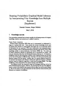
When the domain of a probability distribution is clear from the context, we will omit the under-script to gain in clarity, as in p(x). Another shorthand in notation is that P P x refers to xPX , a sum over all possible values that X can take. For example, the P marginalization rule becomes: p(x) = y p(x, y). Figure 1.1 provides a visual illustration of marginalization in a two-dimensional space. In this example X and Y are two continuous random variables, and their joint distribution p(x, y) is defined as a mixture of two multivariate Gaussian distributions. To marginalize out some random variables (say X), we project the distribution defined over a multi-dimensional space (X × Y) onto a lower-dimensional space (X ), by summing up over the remaining dimensions (Y).

Conditional distributions

By extension to conditional probabilities, a conditional distribution is a probability distribution re-defined over a sub-space of the universe, where the evidence is

1.1

Probability theory

9

p(x|y P [a, b])

p

p(x|y P [c, d])

b

X

a

cd

Y

Fig. 1.2. Conditioning illustration.

true. Any conditional distribution can be derived from a marginal and a joint distribution: p(x, y) p(x|y) = . p(y)

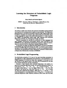
Figure 1.2 provides a visual illustration of conditional distributions in a two-dimensional space. It consists in restricting the domain of p to a particular space where the evidence is true, such as the blue area where y P [a, b], and re-normalizing it accordingly. Then, a proper marginalization can be applied to obtain conditional marginal distributions, like p(x|y P [a, b]).

Independence between random variables

The notion of independence applies to random variables as well. We give right away the definition of conditional independence for multivariate random variables2 . Def. 1.5 Two random variables X and Y are independent given a third random variable Z, conditional denoted X ⊥ ⊥ Y | Z, when the following holds for all (x, y, z) P X × Y × Z: indep.

p(x, y, z)p(z) = p(x, z)p(y, z).

This definition includes univariate random variables as a particular case, for example X = {X}. In that case we may write X ⊥ ⊥ Y | Z as a shorthand for {X} ⊥ ⊥ Y | Z to alleviate our notation. 2

10

Note that most definitions from the literature use the condition p(x, y|z) = p(x|z)p(y|z) or p(x|y, z) = p(x|z), however we prefer the definition below which does not rely on any positivity condition, i.e. p(z) > 0 or p(y, z) > 0.

Chapter 1


p

p

Y

Y

X

X

(a) X and Y are dependent.

(b) X and Y are independent.

Fig. 1.3. Independence between random variables in a two-dimensional space. The joint distributions in (a) and (b) share the same marginal distributions, however only the distribution in (b) factorizes according to its marginals, i.e. p(x, y) = p(x)p(y).

Another random variable of interest is the empty set of variables. By definition, the empty random variable X = ∅ (not to be confused with the empty event E = ∅) is constant, which implies that P (X = x) = 1 for every x P X . If we set Z = ∅ the evidence term above vanishes and we obtain the definition of unconditional independence, i.e. X ⊥ ⊥ Y ⇐⇒ X ⊥ ⊥ Y | ∅. Another implication, called the trivial trivial indep. independence, is that X ⊥ ⊥ ∅ | Z is always true.

Figure 1.3 provides a visual illustration of independence between two continuous random variables. Ex. 1.1 Suppose that we observe a car parking, and that for each car we have access to three information: the fuel level indicator, the battery level indicator, and whether the engine starts when we turn the ignition key. Let us define three binary random variables: X which equals 0 if the car is out of fuel, 1 if not; Y which equals 0 if the car is out of battery, 1 if not; and Z which equals 1 if the engine starts, 0 if not. In this example we will consider the full joint probability distribution given in Table 1.1. The fuel level of a car does not give any information about its battery level, as shown in Table 1.2, and we have that X ⊥ ⊥ Y . However, if we know whether the engine starts or not, the battery level can give an information about the fuel level, and we have X ⊥ 6⊥ Y | Z. For example if the engine does not start when we turn the ignition key, but we have the information that the car is not out of battery, then the car must probably be out of fuel. This is shown in Table 1.3.

car parking example

We may now give an alternative definition of conditional independence between random variables, which is mathematically more convenient. Thm. 1.1 X ⊥ ⊥ Y | Z if and only if there exists two functions f and g such that p(x, y, z) = f (x, z)g(y, z).

1.1

Probability theory

11

Tab. 1.1. The joint probability distribution of X, Y and Z in our car parking example, i.e. p(x, y, z).

Y (battery) 0 1

Z (ignition)

X (fuel)

0

0 1

.06 .13

.23 .06

1

0 1

.00 .01

.01 .50

Tab. 1.2. The joint and marginal probability distributions of X and Y in our car parking example, i.e. p(x, y), p(x) and p(y).

Y (battery) 0 1 X (fuel)

0 1

.06 .14

.24 .56

.20

.80

.30 .70

Tab. 1.3. The joint and marginal conditional probability distributions of X and Y given Z in our car parking example, i.e. p(x, y|z), p(x|z) and p(y|z). Exact probabilities are rounded for clarity. (a)

Z (ignition) 0 X (fuel)

12

Chapter 1

0 1

(b)

Z (ignition)

Y (battery) 0 1 .125 .271

.479 .125

.396

.604

1 .604 .396


X (fuel)

0 1

Y (battery) 0 1 .000 .019

.019 .962

.019

.981

.019 .981

Proof. The first implication X ⊥ ⊥ Y | Z =⇒ ∃(f, g) holds trivially. From Definition 1.5, we readily obtain p(x, y, z) = f (x, z)g(y, z), with f (x, z) = p(x, z) and g(y, z) = p(y|z) when p(z) > 0, any positive value otherwise. To show the converse, let us express p(x, y, z)p(z) and p(x, z)p(y, z) in terms of the f and g functions. We obtain X p(x, y, z)p(z) = f (x, z)g(y, z) f (x0 , z)g(y0 , z), x0 ,y0

as well as   ! X X 0 0 p(x, z)p(y, z) = f (x, z)  g(y , z) g(y, z) f (x , z) , y0

x0

which is equivalent.

1.1.3 Independence models Suppose we are given some conditional (in)dependence statements between random variables, then it would be very convenient if we could derive other (in)dependencies analytically. As we will see, reasoning about conditional independence will prove very useful to learn the structure of probabilistic graphical models from data efficiently, by means of statistical independence tests. To this end, we introduce the notion of independence model, along with an axiomatic characterization of the properties of conditional independence which will provide a formal deductive system. Def. 1.6 An independence model I over a set V consists in a set of triples hX, Y | Zi, called independence relations, where X, Y and Z are disjoint subsets of V and hX, ∅ | Zi and h∅, Y | Zi always belong to I.

indep. model

Consider two independence models I1 and I2 , defined over the same set V. We say that I1 is an independence map for I2 (I-map for short), if all the independence relations in I1 hold in a I2 (I1 Ď I2 ). Equivalently, we say that I1 is a dependence D-map map for I2 (D-map), when all the dependence relations in I1 hold in a I2 (I2 Ď I1 ). P-map Finally, we say that I1 is a perfect map for I2 (P-map), when I1 is both an I-map and a D-map for I2 (I1 = I2 ). I-map

Def. 1.7 A probability distribution p defined over V is said faithful to an independence model I when all and only the independence relations in I hold in p, that is,

faithfulness

hX, Y | Zi P I ⇐⇒ X ⊥ ⊥ Y | Z w.r.t. p.

An independence model I is said probabilistic, if there exists a probability distribution p that is faithful to it.

1.1

Probability theory

13

Conditional independence properties

The study of conditional independence properties goes back to the late seventies with Dawid and Spohn. In seminal theoretical developments, Dawid [Daw79; Daw80] proposes a first axiomatization of conditional independence properties, which unifies a variety of topics within probability and statistics under the same framework. At the same period, Spohn [Spo80] derives similar properties in his work on causal independence. These properties were then studied in great detail by Pearl and colleagues on their work on probabilistic graphical models, work that is presented in [Pea89]. Consider four mutually disjoint random variables, W, X, Y and Z. We first introduce the following properties, which hold in any probability distribution (∧ and ∨ respectively denote the logical AND and OR operators): • Symmetry: hX, Y | Zi ⇐⇒ hY, X | Zi. • Decomposition: hX, Y Y W | Zi =⇒ hX, Y | Zi. • Weak Union: hX, Y Y W | Zi =⇒ hX, Y | Z Y Wi. • Contraction: hX, Y | Zi ∧ hX, W | Z Y Yi =⇒ hX, Y Y W | Zi.

semigraphoid

Any independence model that respects these four properties is called a semi-graphoid [PV87]. A fifth property holds in strictly positive distributions, that is when p > 0: • Intersection: hX, Y | Z Y Wi ∧ hX, W | Z Y Yi =⇒ hX, Y Y W | Zi.

graphoid

Any independence model that respects these five properties is called a graphoid. The term "graphoid" comes from Pearl and Paz [PP86], who noticed that these properties had striking similarities with vertex separation in graphs. Finally, a sixth property will be of particular interest in our work: • Composition: hX, Y | Zi ∧ hX, W | Zi =⇒ hX, Y Y W | Zi.

Any independence model that respects these six properties is called a compositional composi- graphoid [SL14]. Similarly, any semi-graphoid which respects the composition tional property is called a compositional semi-graphoid. The composition property holds

graphoid

14

Chapter 1


in particular probability distributions, such as the regular multivariate Gaussian distribution, or, say, the symmetric binary distributions used in [WMC09].

The characterization problem

As stated previously, any probabilistic independence model satisfies the semi-graphoid properties. Because of that, the semi-graphoid properties provide a necessary condition to characterize probabilistic independence models. It is then possible to detect contradictory conditional independence relations, by checking if they respect the semi-graphoid properties. For example, different experts of the same domain may give different assumptions of conditional independence, which may not correspond together to any probability distribution. The question of the converse implication arises naturally. Do the semi-graphoid properties provide a sufficient condition to characterize a probabilistic independence model? A famous conjecture from Pearl [Pea89], known as Pearl’s completeness conjecture, was that the graphoid axioms were a sufficient condition to characterize probabilistic independence models. Unfortunately, a counter-example was given by Studeny [Stu89], who found a set of conditional independence relations that respects the graphoid axioms, yet does not correspond to any faithful probability distribution. It consists in the following relations, plus the symmetric and trivial ones: hA, B | {C, D}i ∧ hC, D | Ai ∧ hC, D | Bi ∧ hA, B | ∅i.

This counter-example suffices to disprove the conjecture. Moreover, we can see that this example satisfies also the semi-graphoid, the compositional graphoid, and the compositional semi-graphoid axioms, so neither of these sets provides a sufficient condition to characterize probabilistic independence models. Afterwards, Studeny [Stu92] showed that, in the general case, there exists no finite set of conditional independence properties that is both a sufficient and necessary condition to characterize probabilistic independence models. Or, equivalently, probabilistic independence models have no finite complete axiomatic characterization. Later on, Sullivant [Sul09] showed that, even in the restricted case of probabilistic independence models over regular Gaussian distributions, no such characterization exists.

1.1

Probability theory

15

semi-graphoids

independence models

graphoids p

p>0

Fig. 1.4. Overlapping between different classes of independence models. Here p denotes models for which there exists a faithful probability distribution (probabilistic independence models), while p > 0 denotes models for which there exists a faithful strictly positive probability distribution. The compositional classes are omitted for clarity.

As we will see in the Chapter 2, probabilistic graphical models represent independence models in the form of a graph. In the next section we introduce some basic concepts and notations from graph theory which are common to graphical models.

1.2 Graph theory The following definitions are adapted from [SL14; Peñ14]. Formally, a graph G is node defined as an ordered pair of sets (V, E). The first set, V = {V1 , . . . , Vn }, represents edge the nodes (or vertices) of the graph, while the second set E represents its edges. An edge always associates two nodes (not necessarily distinct), called its endpoints. Notice that under this notation our graphs are labeled, that is, every node is considered as a different object. Hence, for example, graph A − B − C is not equal to B − A − C. subgraph

A subgraph of G = (V, E) is any graph G 0 = (V0 , E 0 ) such that V0 Ď V and E 0 Ď E. An induced subgraph is any such subgraph that contains all and only the edges that are present in G between pairs of nodes in V0 .

1.2.1 Connectivity, paths, walks, cycles Two nodes Vi and Vj which are endpoints of the same edge are called adjacent. The adjacents of a set of nodes X in G is the set ADGX = {V1 |V1 is adjacent to V2 in G, V1 6P clique X and V2 P X}. A clique is a set of nodes such that each node is adjacent to every

16

Chapter 1


A

B

C

A

D

B

(a) Undirected.

C (b) Directed.

A

D

B

C

D

(c) Mixed.

Fig. 1.5. Three simple graphs.

other node in the set. A maximal clique is a clique that does not accept any other clique as a proper superset. walk

A walk between two nodes V1 and Vk is a sequence of nodes in the form V1 , . . . , Vk , k ≥ 1, such that Vi is adjacent to Vi+1 for all 1 ≤ i < k. Note that nodes in a walk are not necessarily distinct, i.e. the same node may appear several times. A walk path with only distinct nodes is called a path. A walk with only distinct nodes except cycle V1 = Vk is called a cycle. Within a walk (resp. path) V1 , . . . , Vk , a subwalk (resp. subpath) is any sequence Vi , . . . , Vj , 1 ≤ i ≤ j ≤ k, whose consecutive members appear consecutively in the walk.

connected set

Two nodes that accept a path between them are said connected. A connected set is a set of nodes C such that there is a path between each pair of nodes in C with all intermediate nodes in C. A maximal connected set is a connected that does not accept any other connected set as a proper superset.

1.2.2 Classes of graphs A loop is an edge with the same endpoints, and multiple edges are edges with the same pair of endpoints. A loopless graph is a graph that has no loops. A simple graph simple is a graph that has neither loops nor multiple edges.

loopless

complete

An empty graph is a graph that has no edges. A complete graph is a graph that has connected only one maximal clique. A connected graph is a graph that has only one maximal chordal connected set. A chordal graph is a graph in which every cycle with more than 3 distinct nodes admits a smaller cycle as a proper subset. Classical graphical models are restricted to simple graphs that contain only one type of edge: undirected, in the form X − Y , or directed, in the form X 99K Y . Several attempts have been made to unify and increase the expressiveness of these models, by mixing directed and undirected edges, and by introducing new types of edges such as bi-directed ones in the form X L99K Y . Figure 1.5 provides an illustration of such graphs.

1.2 Graph theory

17

Probabilistic graphical models

2

„

Probability does not exist. — Bruno De Finetti 1974

Probabilistic graphical models belong the the family of probabilistic models, in the sense that they are able to represent a probability distribution p defined over a set of random variables. A PGM always consists in a set of parameters Θ and a graphical structure G. The graphical structure encodes a set of conditional independence relations between nodes in the graph by the presence and absence of edges, and induces an independence model denoted I(G). By definition, p satisfies every independence relations in I(G), that is, hX, Y | Zi P I(G) =⇒ X ⊥ ⊥ Y | Z w.r.t. p. Equivalently, we say that I(G) is an I-map for p. Note that the reverse implication is not required, that is, I(G) is not necessarily a D-map for p. Because p supports the conditional independence relations encoded in the graph, an interesting property of PGMs is that p factorizes according to G. Once this graphical structure is known, the factorization supposedly makes the learning process easier (i.e. choose the best parameters Θ to estimate p from a finite number of samples), as well as the inference process (i.e. answer probabilistic queries from the model). When the graphical structure is unknown, it may also be learned from data samples. The whole process of learning a PGM that estimates a probability distribution p from a finite number of samples is usually split into two distinct problems, namely the structure learning problem (learn G), and the parameter learning problem (learn Θ).

generative vs discriminative

Probabilistic models, among which are PGMs, may be further divided into two categories: generative models, which encode a probability distribution p(v) over a set of random variables V, and discriminative models, which encode a conditional probability distribution p(y|x) over two disjoint sets of random variables X and Y. This chapter will focus on the former family of generative models, as discriminative models may be seen as a particular case of these.

19

2.1 Classical graphical models We will now review the most popular models based on undirected graphs (Markov networks) and acyclic directed graphs (Bayesian networks). We will extend the discussion to advanced graphical models in the next section. Note that the literature abounds with different families of graphical models, and the list we discuss here is by far non-exhaustive.

2.1.1 Undirected graphs The most popular probabilistic models based on undirected graphs are the Markov networks (MNs), also called Markov random fields, which emerged from different fields in the literature. Historically, the theory of Markov fields traces back to the Ising model [Isi25] from statistical physics, where undirected graphs were used to model geometric arrangements in space. Several types of Markov conditions were later introduced (see Lauritzen [Lau96] for an overview) in order to associate these graphs with independence models.

Undirected graphs as probabilistic models

Def. 2.1 A Markov network consists in a set of random variables V = {V1 , . . . , Vn }, a simple Markov undirected graph G = (V, E), and a set of parameters Θ. Together, G and Θ define a network probability distribution p over V which factorizes as Y

p(v) =

φi (ci ),

Ci PCl G

where Cl G is the set of all cliques in G. Each φi function is called a factor, a potential function, or a clique potential. Note that, without loss of generality, the factorization of p(v) may also be defined over the maximal cliques in G. Ex. 2.1 Consider the undirected graphs in Figure 2.1. From the above definition, the corresponding factorizations over the maximal cliques are p(v) = φ1 (a, b)φ2 (b, c)φ3 (c, d)φ4 (d, a) in (a), and p(v) = φ1 (a, b, d)φ2 (d, b, c) in (b). Suppose that A, B, C and D are 4 binary variables, then Tables 2.1 and 2.2 respectively define valid clique potentials for each of these Markov network structures. These potentials are valid because their P product defines a valid probability distribution, that is, a,b,c,d p(a, b, c, d) = 1. Note however that individual clique potentials do not necessarily normalize to 1, and therefore do not necessarily correspond to marginal or conditional probability distributions.

20

Chapter 2


Because of this, potential functions in Markov network are not subject to an intuitive probabilistic interpretation, and one must always go through a factorization to obtain proper probability measures.

Undirected graphs as independence models

Every undirected graph G induces a formal independence model I(G) over V, by means of a graphical separation criterion, called u-separation. Def. 2.2 Given an undirected graph G, I(G) is the independence model such that a disjoint UG ind. triplet hX, Y | Zi belongs to I(G) iff Z u-separates X and Y in G, that is, every path model between a node in X and a node in Y contains a node in Z.

Note that the trivial relations hX, ∅ | Zi and h∅, Y | Zi are included in I(G). From the above definition, the two extreme independence models correspond to the empty graph (without edges), where I(G) contains every possible triplet, and the clique graph where I(G) contains only trivial relations. Indeed, in undirected graphical models the addition of edges only creates dependence relations, while their removal creates independence relations. Ex. 2.2 Consider again the undirected graphs in Figure 2.1. In (a) the independence model is h{A}, {C} | {D, B}i ∧ h{D}, {B} | {A, C}i, while in (b) it reduces to h{A}, {C} | {D, B}i by the addition of a single edge.

The next example illustrates u-separation in more complicated cases. Ex. 2.3 Consider the undirected graph in Figure 2.2. Here the independence model contains h{A}, {B} | {C}i because every path between A and B contains C, as well as h{A}, {B, F } | {C, E}i because every path between A and B or between A and F contains C. However, the relation h{A}, {B, F } | {D, E}i is not in I(G) because there is a path between A and B which contains neither D nor E.

Soundness of Markov networks

A Markov network structure always defines an I-map of the underlying probability distribution. Consider G an undirected graph over the variables V, and p a probability distribution over the same set. Thm. 2.1 I(G) is an I-map for p if p factorizes into a product of potentials over the cliques in G.

2.1 Classical graphical models

21

A

A

D

B

D

B

C

C

(a)

(b)

Fig. 2.1. Two undirected graphs (UGs).

Tab. 2.1. A set of clique potentials (i.e. parameters Θ) that define a valid probability distribution according to the Markov network structure in Figure 2.1a. (a) φ1 (a, b)

(b) φ2 (b, c)

B 0 1

A

C

0

1

2/3 1/3

3/3 1/3

B

(c) φ3 (c, d)

0 1

0

1

1/2 1/2

2/2 3/2

(d) φ4 (d, a)

D 0 1

C

A

0

1

3/3 2/3

2/3 1/3

D

0 1

0

1

3/10 1/10

1/10 2/10

Tab. 2.2. A set of clique potentials (i.e. parameters Θ) that define a valid probability distribution according to the Markov network structure in Figure 2.1b. (a) φ1 (a, b, d)

(b) φ2 (b, c, d)

B

B

A

D

0

1

C

D

0

1

0

0 1

1/8 1/8

3/8 1/8

0

0 1

1/6 1/6

4/6 1/6

1

0 1

2/8 2/8

1/8 2/8

1

0 1

1/6 2/6

2/6 3/6

A

B

D

C

Fig. 2.2. An undirected graph to illustrate u-separation.

22

Chapter 2


E

F

Proof. Let X, Y, Z be any three disjoint subsets of V such that hX, Y | Zi P I(G). We start by considering the case where X Y Y Y Z = V. As Z u-separates X and Y, there are no direct edges between X and Y. Hence, any clique in G is fully contained either in X Y Z or in Y Y Z. So we may re-write the factorization of p as p(v) =

Y i

φi (ci ) ·

Y

φj (cj ),

j

where i indexes of the set of cliques that are contained in X Y Z, while j indexes the remaining cliques. As discussed, none of the factors in the first product involves any variable in Y, and none in the second product involves a variable in X. Hence we can rewrite this product as p(v) = f (x, z)g(y, z). The desired independence relation follows immediately (Theorem 1.1), that is, X ⊥ ⊥ Y | Z. In the case where X Y Y Y Z Ă V, let us to consider the remaining set of variables W = V \ (X Y Y Y Z) as follows. Necessarily, one can find a partition {W1 , W2 } of W such that Z u-separates X Y W1 and Y Y W2 in G. Using our precedent argument, we have that X Y W1 ⊥ ⊥ Y Y W2 | Z. Using the decomposition property (from the semi-graphoid axioms), we obtain the desired result X ⊥ ⊥ Y | Z.

The converse implication was shown to be true only for strictly positive distributions1 . This result is known as the Hammersley-Clifford’s theorem [HC71]. Thm. 2.2 Suppose that p > 0. Then, p factorizes into a product of potentials over the cliques in G Hammersley iff I(G) is an I-map for p. Clifford

Interestingly, Hammersley and Clifford found the positivity condition p > 0 unnatural, and postponed their publication in hope of relaxing it. Thereby, they were preceded by Besag [Bes74] in publishing the theorem. The condition was shown to be necessary shortly after by Moussouris [Mou74], who provided a simple counter-example with only 4 variables, which we present below. Ex. 2.4 Consider 4 binary variables A, B, C, D, and the probability distribution in Table 2.3. The undirected graph in Figure 2.1a is an I-map for p, because A ⊥ ⊥ C | {B, D} and B ⊥ ⊥ D | {A, C}. However, one may observe that each combination of {A, B}, {B, C}, {C, D} or {D, A} has a positive probability, while some joint combinations of {A, B, C, D} have zero probabilities. The only way to obtain a zero probability for a particular joint combination would be to set one of the clique potentials φ1 ({a, b}), φ2 ({b, c}), φ3 ({c, d}) or φ4 ({d, a}) to zero, which would immediately result in a zero probability for the corresponding pairwise combination. Thus, p cannot be encoded as a product of pairwise potentials. 1

Note that, in the discrete case, Geiger et al. [GMS02] give a necessary and sufficient condition that encompasses the positivity condition from the Hammersley-Clifford’s theorem.


23

Tab. 2.3. Moussouris’ counter-example of a probability distribution that satisfies the independence relations in a grid graph (Figure 2.1) but cannot be encoded as a product of pairwise potentials. Any {a, b, c, d} combination that is not displayed has probability 0. This distribution does not satisfy the positivity condition.

A

B

C

D

p(a, b, c, d)

0 0 0 0 1 1 1 1

0 0 0 1 1 1 1 0

0 0 1 1 1 1 0 0

0 1 1 1 1 0 0 0

1/8 1/8 1/8 1/8 1/8 1/8 1/8 1/8

The Hammersley-Clifford’s theorem has a practical application for Markov network structure learning. Assuming p > 0, learning a Markov network that estimates p can be done in two steps: 1) find a structure G that is an I-map for p; and 2) learn clique potentials φi that express p. Without the positivity condition, it is not guaranteed that the graph recovered after phase 1) will be able to correctly encode p.

Conditional independence properties of undirected graphs

Any independence model that can be expressed by u-separation over an undirected graph, i.e. for which there exists an undirected graph G that is a perfect map, is said UG-faithful. An interesting property of such independence models is that they are characterized by a finite set of conditional independence properties, as shown by Pearl and Paz [PP86]. Thm. 2.3 Consider an independence model I defined over V. A necessary and sufficient condition for I is to be UG-faithful is that it satisfies the following properties: • Symmetry: hX, Y | Zi ⇐⇒ hY, X | Zi. • Decomposition: hX, Y Y W | Zi =⇒ hX, Y | Zi. • Intersection: hX, Y | Z Y Wi ∧ hX, W | Z Y Yi =⇒ hX, Y Y W | Zi. • Strong union: hX, Y | Zi =⇒ hX, Y | Z Y Wi. • Transitivity, ∀W P W: hX, Y | Zi =⇒ hX, W | Zi ∨ hW, Y | Zi.

24

Chapter 2


Note that we can easily derive the weak union, contraction and composition properties from this set of axioms, and as a consequence independence models based on undirected graphs are compositional graphoids. First, weak union may be derived as follows: hX, Y Y W | Zi implies hX, Y | Zi due to the decomposition property, which in turn implies hX, Y | Z Y Wi due to the strong union property. Second, contraction is derived as follows: hX, Y | Z Y Wi ∧ hX, W | Zi implies hX, Y | Z Y Wi ∧ hX, W | Z Y Yi due to the strong union, which in turn implies hX, Y Y W | Zi due to the intersection. Finally, composition is derived as follows: hX, Y | Zi ∧ hX, W | Zi implies hX, Y | Z Y Wi ∧ hX, W | Z Y Yi due to the strong union, which in turn implies hX, Y Y W | Zi due to the intersection. A second important property of undirected graphs is that they always produce a probabilistic independence model. Indeed, it was shown by Geiger and Pearl [GP90] that for every independence model I that is UG-faithful, there exists a probability distribution p that satisfies all and only the independence relations in I. However, the converse does not necessarily hold, that is, not every probability distribution p is UG-faithful. Because of the axiomatic characterization given above, all and only the distributions that satisfy the intersection, the strong union and the transitivity property are UG-faithful.

Discussion

We will now emphasize some important points and caveats about Markov networks. First, any probability distribution can be encoded in a Markov network. It suffices to consider the complete graph G, which does not impose any constraint on the expression of p, that is, p(v) = φ(v). With a proper parameterization, φ may encode any probability distribution, even a non-strictly positive one such as in Example 2.4. However, it must be kept in mind that the benefit of modeling a probability distribution with a Markov network comes from the sparseness of structure. The key idea of probabilistic graphical models is the factorization of p, which makes the learning and inference problems easier. This factorization comes from the independence relations encoded in the model, which for Markov networks directly result from the sparseness of the structure (recall that the absence of an edge only creates independence relations). The tractability of graphical models is often measured in terms of the tree-width of the model, which for undirected graphical models is given by the size of the largest clique, after the graph has been made chordal with added edges. Another way of assessing the tractability of a model is by measuring the number of degrees of freedom in its parameterization. Indeed, the more the


25

structure of a model imposes restrictions on p, the less free parameters remain to express p, and the easier will be the learning and inference problems. Ex. 2.5 Consider 3 binary random variables A, B and C. Their joint distribution can be represented as a contingency table in 3 dimensions, resulting in 23 parameters. Obviously one of these parameters is not free, as it can be deduced from the others due to the P normalization a,b,c p(a, b, c) = 1. Still, we have 23 − 1 = 7 free parameters to express p. If p supports some independence relations, such as A ⊥ ⊥ C | B, then it factorizes as p(a, b, c) = p(a, b)p(c|b), in which case the number of free parameters is reduced to 5 (22 − 1 for p(a, b) plus 2 × (21 − 1) for p(c|b)). This corresponds to the undirected graph A − B − C with p(a, b, c) = φ1 (a, b)φ2 (b, c). In the extreme case where every single variable is independent of the others, we have p(a, b, c) = p(a)p(b)p(c), in which case the number of free parameters is reduced to 3. This corresponds to the empty graph A B C (without edges), with p(a, b, c) = φ1 (a)φ2 (b)φ3 (c).

To summarize, for a graphical model to be interesting it should include as many of the independence relations in p as possible. However, the model must remain an I-map of p, that is, all the independence relations encoded in the structure must hold in p. In the case where p is UG-faithful, then there exists an "optimal" Markov network in some sense, that is, an undirected graphical model that perfectly encodes all and only the independence relations in p. However, and this is the main flaw of undirected graphical models, not every probability distribution is UG-faithful. That is, there are some probability distributions for which it is impossible to include all the independence relations in an undirected graph without violating a dependence relation as well. Ex. 2.6 Consider again the car parking example from Example 1.1. It can be verified that the only non-trivial independence relation is X ⊥ ⊥ Y . Then, p factorizes as p(x, y, z) = p(x)p(y)p(z|x, y), which corresponds to 6 free parameters. Unfortunately, this factorization can not be exploited within an undirected graphical model. Indeed, any undirected model that encodes the relation hX, Y | ∅i necessarily implies hX, Y | Zi as well, due to the strong union property (Theorem 2.3). As a result, the only undirected graph that is an I-map for p is the complete graph, which necessarily results in 7 free parameters. In such a situation Markov networks do not appear to be well suited models to encode p.

In the next section we will introduce directed acyclic graphical models, which have admittedly a higher expressive power that undirected models. However, directed acyclic models do not subsume undirected ones, as they suffer from different flaws and in some cases an undirected independence model is still better suited than a directed one.

26

Chapter 2


Fig. 2.3. A path diagram from Wright [Wri20], showing how the fur pattern of the litter guinea pigs is determined by various genetic and environmental factors.

2.1.2 Directed acyclic graphs Within classical probabilistic graphical models, the directed counterpart of Markov networks are the Bayesian networks (BNs), which rely on directed acyclic graphs (DAGs). The modern definition of Bayesian networks as probabilistic independence models originates from the mid-1980s in a series of papers from Pearl and his colleagues [Pea85; VP88; GP88; GVP89; GVP90], work that is presented in great detail in Pearl [Pea89]. However, the idea of using directed acyclic graphs to encode general probability distributions goes back to the mid-1970s with influence diagrams in the context of decision analysis [HM81]. Furthermore, a first use of directed graphs to represent relations between random variables can be traced back to the 1920s with Wright [Wri20; Wri34] who introduced the notion of path diagrams in the context of genetics analysis (Figure 2.3).

Before talking about Bayesian networks, we must introduce some notions from graph theory that are specific to directed graphs. Recall that a directed graph G = (V, E) parent contains only edges in the form Vi 99K Vj . The parents of a set of nodes X is the set child PAG = {V1 |V1 99K V2 is in G, V1 6P X and V2 P X}. Likewise, the children of X is the X set CHGX = {V1 |V1 L99 V2 is in G, V1 6P X and V2 P X}. When clear from the context we may omit the superscript and just write PAX and CHX .

A directed walk from V1 to Vk is a walk V1 , . . . , Vk such that Vi P PAVi+1 for all 1 ≤ i < k. Likewise, the definition of directed path and directed cycle follows. The ancestors ancestor of X is the set ANX = {V1 |V1 , . . . , Vk is a directed path in G, V1 6P X and Vk P X}. descendant Likewise, the descendants of X is the set DEX = {V1 |Vk , . . . , V1 is a directed path in G, V1 P 6 X and Vk P X}, and the non-descendants of X is the set NDX = V \ (X Y DEX ).


27

directed acyclic graph

A directed acyclic graph (DAG for short) is a directed graph that contains no directed cycle. An equivalent characterization is a directed graph in which no node is both an ancestor and a descendant of the same node, that is, ANV X DEV = ∅ for every V P V. Some authors point that the phrase directed acyclic graph is ambiguous, and prefer to refer to acyclic directed graphs (ADG), or acyclic digraphs [Stu05, p. 46]. In this work we will follow the common practice in the field of Bayesian networks and refer to DAGs.

Directed acyclic graphs as probabilistic model

Def. 2.3 A Bayesian network consists in a set of random variables V = {V1 , . . . , Vn }, a simple Bayesian directed acyclic graph G = (V, E), and a set of parameters Θ. Together, G and Θ define network a probability distribution p over V which factorizes as p(v) =

Y

p(vi |paVi ).

Vi PV

chain rule for BNs

This factorization according to a DAG is called recursive factorization, or chain rule for BNs. Each of the factors p(vi |paVi ) can be seen as a potential function φi (vi , paVi ), similarly to a clique potential in Markov networks. However, in Bayesian networks each factor must define a valid conditional probability distribution for Vi , and thus P respects the normalization constraint vi φi (vi , paVi ) = 1.

Ex. 2.7 Consider the DAGs in Figure 2.4. From the above definition, the corresponding factorizations are p(v) = p(a)p(d|a)p(b|a)p(c|b, d) in (a) and p(v) = p(a)p(d|a)p(b|a, d)p(c|b, d) in (b). Suppose that A, B, C and D are 4 binary variables, then Tables 2.4 and 2.5 respectively define valid conditional probability distributions for each of the Bayesian networks. In the context of discrete random variables, such tables are called conditional probability tables (CPTs). Note that each of these conditional probability distribution is normalized and can be intuitively interpreted. For example, from Table 2.4b we have that the event D = 0 is more likely to happen if we already know that A = 0 (probability 0.6), than when we know that A = 1 (probability 0.5).

Directed acyclic graphs as independence models

Every DAG G induces a formal independence model I(G) over V, by means of a graphical separation criterion called d-separation [GVP90]. In order to define collider d-separation, we must first introduce the notion of a collider node. Within a path V1 , . . . , Vk , an intermediate node Vi is said to be a collider iff it is in the form Vi−1 99K Vi L99 Vi+1 .

28

Chapter 2


A

A

D

B

D

B

C

C

(a)

(b)

Fig. 2.4. Two directed acyclic graphs (DAGs).

Tab. 2.4. A set of conditional probability tables that define a valid set of parameters Θ for the Bayesian network structure in Figure 2.4a. (a) p(a)

(b) p(d|a)

D

A 0

1

0.4

0.6

0 1

A

(c) p(b|a)

0

1

0.6 0.5

0.4 0.5

(d) p(c|b, d)

B

A

0 1

C

0

1

B

D

0

1

0.3 0.1

0.7 0.9

0

0 1

0.8 0.7

0.2 0.3

1

0 1

0.5 0.7

0.5 0.3

Tab. 2.5. The conditional probability table p(b|a, d) that, along with Tables 2.4a, 2.4d and 2.4b, define a valid set of parameters Θ for the Bayesian network structure in Figure 2.4b.

B A

D

0

1

0

0 1

0.2 0.5

0.8 0.5

1

0 1

0.0 0.2

1.0 0.8


29

Def. 2.4 Given an DAG G, I(G) is the independence model such that a disjoint triplet hX, Y | Zi DAG ind. belongs to I(G) iff Z d-separates X and Y in G, that is, every path between a node in model X and a node in Y contains a non-collider node that belongs to Z, or a collider node that does not belong to Z Y ANZ . Again, the trivial relations hX, ∅ | Zi and h∅, Y | Zi are included in I(G). Note that some authors propose a different definition of I(G) with the moralization criterion, which was shown to be equivalent to the d-separation criterion [Lau+90]. From the above definition, d-separation is equivalent to u-separation when G contains v-structure no v-structure, that is, no pattern in the form V1 99K V2 L99 V3 with V1 and V3 non-adjacent. Ex. 2.8 Consider again the DAGs in Figure 2.4. In (a) the induced independence model is h{A}, {C} | {D, B}i∧h{D}, {B} | {A}i. This is different from the independence model induced from the undirected graph in Figure 2.1a, due to the v-structure D 99K C L99 B. In (b) the independence model is h{A}, {C} | {D, B}i, which is equivalent to the one from the undirected graph in Figure 2.1b since here the DAG contains no v-structure. Similarly to the undirected case, the two extreme independence models correspond to the empty graph (without edges), where I(G) contains every possible triplet, and a clique graph (without directed cycle), where I(G) contains only trivial relations. Indeed, the addition of edges in a DAG only creates dependence relations, while their removal creates independence relations. A friendly interpretation of d-separation is the following. Consider a path between two random variables X and Y , and a conditioning set Z. The path represents an information flow. When Z is empty, each intermediate node that is not a collider is open, that is, it lets the flow go through. Conversely, each intermediate node that is a collider is closed, and blocks the flow. By adding some observed variables to Z, one can only change the state of non-collider nodes from open to closed, and collider nodes from closed to open. When a non-collider node along the path is known (i.e. added to Z) it becomes closed, and when a collider node or one of its descendants is known it becomes open. One then simply has to check if, given Z, all the nodes along the path are open to determine if there is an information flow between X and Y . In that case the path is said active, and Z does not d-separate X and Y . Ex. 2.9 Consider the DAG in Figure 2.5. While in this graph the adjacencies are the same as in the undirected graph in Figure 2.2, the independence model is different due to the v-structure A 99K C L99 D. Here the independence model contains h{A}, {B} | {C}i because the only path A 99K C 99K B is closed by the non-collider C that is observed. However, it does not contain h{A}, {B, F } | {C, E}i because in the path A 99K C L99 D 99K F the non-collider D is open, as well as the collider C that is observed. Other interesting relations induced by G are h{A}, {F } | ∅i 6P I(G), because of the open path

30

Chapter 2


A

B

D

C

E

F

Fig. 2.5. A directed acyclic graph to illustrate d-separation.

A 99K C 99K E 99K F . Conditioning on E does not d-separate A and F either, it closes the previous path but opens a new one with A 99K C 99K E L99 D. We may then add C to the conditioning set, which closes the two previous paths but opens yet a new one with A 99K C L99 D 99K F . We may now add D, which ultimately closes every path, and finally notice that conditioning on {C, D} is sufficient and that E it no longer necessary in the conditioning set.

Soundness of Bayesian networks

As with Markov networks, a Bayesian network structure always defines an I-map of the underlying probability distribution. Moreover, the converse implication is true (recall that for MNs the converse holds only when p > 0). Consider G a directed acyclic graph graph over the variables V, and p a probability distribution over the same set. Thm. 2.4 With G a DAG, I(G) is an I-map for p iff p factorizes recursively over G.

Proof. We first prove the implication I-map =⇒ factorization. Because G is a DAG, we may arrange its nodes in a topological ordering V1 , . . . , Vn according to G, that is, i < j if Vi 99K Vj is in G. From the chain rule of probabilities, we can write p as p(v) =

n Y

p(vi |v1 , . . . , vi−1 ).

i=1

Now, consider one of the factors p(vi |v1 , . . . , vi−1 ). From the d-separation criterion, every node is independent of its non-descendants given its parents (a.k.a. local Markov property), that is, Vi ⊥ ⊥ NDVi \ PAVi | PAVi . Because of our ordering of the nodes, all of Vi ’s parents are necessarily in the set {V1 , . . . , Vi−1 }, while none of its descendants can possibly be in the set. Then, we can write {V1 , . . . , Vi−1 } = W Y PAVi , with W Ď (NDVi \ PAVi ). From the decomposition property we obtain Vi ⊥ ⊥ W | PAVi , which implies p(vi |v1 , . . . , vi−1 ) = p(vi |paVi ).


31

By applying this transformation to every such factor, we obtain the desired recursive factorization according to G.

Second, we prove the converse. Let X, Y, Z be any three disjoint subsets of V such that hX, Y | Zi P I(G). As Z d-separates X and Y, there are no direct edges between X and Y. Hence, the variables in X have no parent in Y and the variables in Y have no parent in X. Moreover, there are no pattern in the form X 99K Z L99 Y with X P X, Z P Z and Y P Y, so the variables in Z have either no parent in X or no parent in Y. Let us now introduce C, the set of all the remaining variables that have no descendant in X Y Y Y Z. In the case where X Y Y Y Z Y C = V, we may re-write the factorization of p as Y

p(v) =

Y

p(vi |paVi ) ·

Vi PX Y(Z X CHX )

p(vj |paVj ) ·

Y

p(vl |paVl ).

Vl PC

Vj PY Y(Z\CHX )

As discussed, none of the factors in the first product involves any variable in Y Y C, and none in the second product involves any variable in X Y C. Let us now marginalize out C, we obtain p(x, y, z) = f (x, z)g(y, z) ·

X Y

p(vl |paVl ).

c Vl PC

Consider C1 , . . . , Ck an arrangement of the nodes in C in a topological ordering according to G. Then, the third term transforms to a recursive sum X

p(c1 |paC1 ) · · · · ·

c1

X

p(ck |paCk ).

ck

The right-most term sums to 1 because of the normalization constraint, and vanishes. By summing each remaining term from right to left, the whole expression equals 1 and we obtain p(x, y, z) = f (x, z)g(y, z). The desired independence follows immediately (Theorem 1.1), that is, X ⊥ ⊥ Y | Z. In the case where X Y Y Y Z Y C Ă V, let us to consider the remaining set of variables W = V \ (X Y Y Y Z Y C) as follows. Necessarily, one can find a partition {W1 , W2 } of W such that Z d-separates X Y W1 and Y Y W2 in G. Suppose it is not the case, then there is a node W P W such that hX, {W } | Zi 6P I(G) and h{W }, Y | Zi 6P I(G). Equivalently, there is an open path P1 = (X, . . . , V, . . . , W ) between a node X P X and W , and an open path P2 = (Y, . . . , V, . . . , W ) between a node Y P Y and W , with V, . . . , W the shared sequence between P1 and P2 (of size 1 at least in the case where V = W ). Because hX, Y | Zi P I(G), the path P3 = (X, . . . , V, . . . , Y ) is closed, so V is a collider node in P3 that is not in Z nor has any descendant in Z. This implies that V has no descendant in X or Y either, otherwise this would result in an open path between X and Y. Hence, V belongs to C. This also implies that V is not a collider in P1 ,

32

Chapter 2


otherwise the path would be closed. Moreover, there can be no collider node along the path V, . . . , W , otherwise it would be a descendant of V without a descendant in Z, and the path P1 would be closed. So either W is a descendant of V , or W = V . In both cases W also belongs to C, which violates our initial assumption W P W.

W P1

X ... ...

...

P2

V

... ...

Y

P3

Using our precedent argument we have that X Y W1 ⊥ ⊥ Y Y W2 | Z. Using the decomposition property we obtain the desired result X ⊥ ⊥ Y | Z.

Conditional independence properties of directed acyclic graphs

Any independence model that can be expressed by d-separation over a directed acyclic graph (i.e. for which there exists a DAG G that is a perfect map) is said to be DAG-faithful. Unlike in the case of undirected graphs, it was shown that such independence models can not be characterized by a finite set of conditional independence properties [Gei87; Li08; WWL02]. However, such a finite set of axioms can provide a necessary condition for an independence model to be faithful to a DAG. Pearl [Pea89] gives such a partial characterization. Thm. 2.5 Consider an independence model I defined over V. A necessary condition for I to be DAG-faithful is that it satisfies the following properties: • Symmetry: hX, Y | Zi ⇐⇒ hY, X | Zi. • Decomposition: hX, Y Y W | Zi =⇒ hX, Y | Zi. • Weak Union: hX, Y Y W | Zi =⇒ hX, Y | Z Y Wi. • Contraction: hX, Y | Zi ∧ hX, W | Z Y Yi =⇒ hX, Y Y W | Zi. • Intersection: hX, Y | Z Y Wi ∧ hX, W | Z Y Yi =⇒ hX, Y Y W | Zi.


33

• Composition: hX, Y | Zi ∧ hX, W | Zi =⇒ hX, Y Y W | Zi. • Weak transitivity, ∀W P W: hX, Y | Zi ∧ hX, Y | Z Y W i =⇒ hX, W | Zi ∨ hW, Y | Zi. • Chordality, ∀(X, Y, Z, W ) P X × Y × Z × W: hX, Y | {Z, W }i ∧ hZ, W | {X, Y }i =⇒ hX, Y | W i ∨ hX, Y | Zi. As a direct consequence, DAG-faithful independence models are compositional graphoids. Moreover, as in the undirected case, an important property of directed acyclic graphs is that they always produce a probabilistic independence model. Indeed, it was shown by Geiger and Pearl [GP88] that for every independence model I that is DAG-faithful, there exists a probability distribution that satisfies all and only the independence relations in I. However, here again the converse does not necessarily hold, that is, not every probability distribution is DAG-faithful.

A note on causal networks

We now briefly discuss the idea of causality and causal networks, although this is not required for the understanding of our work. We find necessary to add some clarifications to highlight the difference between a Bayesian network and a causal network, since many people do not distinguish between the two notions and tend to interpret every DAG as a causal graph. Causal networks are basically Bayesian networks whose structure can be given a causal interpretation, that is, each directed edge represents a direct causal influence between a cause and an effect. Causal networks offer a powerful tool for reasoning about the causal influences among a set of random variables. A well-known paradox in statistics that is well explained with a causal DAG is the so-called Simpson’s paradox, first described in Simpson [Sim51]. Ex. 2.10 Consider a population of people who have the same disease, and among which some took a treatment, and some recovered the disease. Take three binary random variables G, T and R that respectively correspond to three indicators for each individual: his gender g P {male, f emale}, he took a treatment t P {yes, no}, and whether or not he recovered from the disease r P {yes, no}. Let us observe 200 people randomly, 100 male and 100 female, which results in the probability distribution given in Table 2.6. We ask the following question: is the treatment efficient? In the general case, people who took the treatment tend to recover more: p(R = yes|T = yes) > p(R = yes|T = no).

Simpson’s paradox (1/2)

34

Chapter 2


Tab. 2.6. Illustration of Simpson’s paradox. This table represents the joint probability distribution of G (gender), T (treatment) and R (recovery) on a population of 200 people (100 male and 100 female). #(g, t, r) counts the number of people that have characteristics (g, t, r) in the population, while p(r|g, t) and p(r|t) the corresponding conditional probability distributions.

R (recovery) no yes

T (treatment)

G (gender)

no

yes

no

male female

42 06

28 24

.60 .20

yes

male female

24 21

06 49

.80 .30

#(g, t, r)

no

yes

.40 .80

.48

.52

.20 .70

.45

.55

p(r|g, t)

p(r|t)

However, it also appears that women who took the treatment tend to recover less: p(R = yes|T = yes, G = f emale) < p(R = yes|T = no, G = f emale). And, very surprisingly, the same phenomenon appears in the population of men: p(R = yes|T = yes, G = male) < p(R = yes|T = no, G = male). All these statements appear to be true according to p, but are rather counter-intuitive, hence the paradox. Let us to give it an explanation with a causal DAG. Suppose the causal DAG in Figure 2.6a represents the causal mechanisms between our three random variables. Admittedly, the causal directions in the DAG are plausible: the gender is determined when people are born thus can not be an effect of taking the treatment or recovering the disease, and the treatment is taken before the recovery in time thus can not be an effect of it. We may now re-formulate our initial question more explicitly, that is: does the action of taking the treatment has a positive causal effect on the recovery of the disease? When measuring the probability p(r|t), two information paths are open in the graph (in the sense of d-separation): the direct causal path T 99K R and the indirect non-causal path T L99 G 99K R due to the common cause G. Suppose the direct influence T 99K R is negative (taking the medicine has a negative effect on the recovery), then the statistical relationship carried in the first path is negative. At the same time, suppose the direct influences G 99K T and G 99K R are both positive (women tend to consume more medicine than men, and women naturally tend to recover the disease better than men), then the statistical relationship carried in the second path is positive as well (people who have taken the treatment tend to be women, who tend to recover better, so overall people who have taken medicine tend to recover better). When measuring the conditional probability p(r|t), the statistical relationships carried in the two paths are mixed up, which results in a negative or a positive relationship depending on which path is the strongest. In the present situation the overall statistical relationship is positive. However, it can not be given any causal meaning since it carries information from the non-causal


35

G

T

B

R (a)

T

R (b)

Fig. 2.6. Two causal DAGs illustrating Simpson’s paradox.

path T L99 G 99K R. The second measurement p(r|t, g) adds G to the conditioning set, which closes the non-causal path T L99 G 99K R owing to the d-separation criterion. Because of that, only the causal path T 99K R remains, and the resulting statistical measurements can be interpreted as a causal relationships. So, with this causal DAG, it is the second set of measurements (consider men and women separately) that answers our initial question. The answer is then no, the treatment does not have a positive causal effect on the disease recovery.

By modeling Simpson’s paradox with a causal DAG, we can measure unambiguously the causal influence between two random variables, by choosing a proper conditioning set Z that closes every non-causal path in the DAG and keeps every causal path open between the variables of interest. This measurement is known as the do-calculus do-calculus [Pea95; Pea12], which is nowadays a well established tool for causal inference. It consists in measuring the probability of observing an event given that an action is performed, denoted p(x|do(y)). This is different from p(x|y), i.e. the probability of observing an event given that another event is observed. In do-calculus, the structure of a causal DAG tells us how to compute p(x|do(y)). In Example 2.10, P we have p(r|do(t)) = g p(g)p(r|g, t) because of the common cause G. In that case G is commonly called a confounding variable. We can now measure the causal influence from T to R unambiguously, which gives p(R = yes|do(T = no)) = 0.60 and p(R = yes|do(T = yes)) = 0.45. We end up with the same conclusion we had reached in Example 2.10. In Example 2.10, the direction of the edges was justified only by introducing some external knowledge, a.k.a. the expert knowledge. Without an expert to validate that the DAG structure indeed corresponds to a plausible causal system, no causal interpretation can be given to the measured probabilities. When someone tries to infer a causal explanation from observational data, that person always implicitly enforces an underlying causal system. If that causal system is wrong, such interpretations can lead to perilous conclusions. Ex. 2.11 Consider the same probability distribution as in Example 2.10, but suppose that the Simpson’s variable G is replaced with the variable B, b P {low, high} representing the blood paradox pressure level of each individual. The probability distribution is exactly the same, (2/2)

36

Chapter 2


however now the causal DAG could arguably be the one in Figure 2.6b. From our external knowledge, the blood pressure is more likely to be a consequence than a cause of taking the treatment. If we apply the do-calculus again to assess the efficiency of the treatment, then we have this time p(r|do(t)) = p(r|t) due to the causal structure of the DAG. This gives p(R = yes|do(T = no)) = 0.52 and p(R = yes|do(T = yes)) = 0.55, and we conclude that the treatment has a positive causal effect on the recovery of the disease. Same observational data, different causal system, different causal interpretation.

It is important to keep in mind that it is impossible to infer causal mechanisms from observational data. It is not because a Bayesian network correctly encodes a probability distribution p, even faithfully, that the corresponding DAG necessarily represents causal mechanism that generated the data. Indeed, the two DAGs in Figure 2.6 are able to faithfully encode the probability distribution from Table 2.6. Without any additional information, both DAGs are indistinguishable with respect to the observed data, and represent equally plausible causal systems. However, performing do-calculus with these two DAGs does not lead to the same conclusions. In the general case, it is impossible to infer causal relationships from a probability distribution based on observational data. The only way to infer such relationships is by collecting experimental data, that is, performing an action on the system and observe how it affects the probability distribution. This is well-known in the domain of clinical studies, as one can assess the effectiveness of a treatment only through double-blind trials (a.k.a. placebo-controlled studies). Readers interested in causality may consult Dawid [Daw10], or the very comprehensive book from Pearl [Pea09].

Discussion

We will now compare directed acyclic and undirected graphical models, namely Bayesian networks and Markov networks. We first discuss how Bayesian networks are similar to Markov networks, and finally we emphasize on their differences. First, just like Markov networks, any probability distribution can be encoded in a Bayesian network. Consider an arbitrary ordering V1 , . . . , Vn of the nodes, and the complete DAG such that Vi 99K Vj for every j > i. Then, the recursive factorization according to the DAG is p(v) = p(v1 )p(v2 |v1 ) . . . p(vn |v1 , . . . , vn−1 ), which respects the chain rule of probability and does not impose any constraint on p. This holds for any ordering of the nodes, and thus any complete DAG.


37

However, just like Markov networks, the structure of a Bayesian network should be as sparse as possible. This is true for probabilistic graphical models in general, and neither Markov networks or Bayesian networks are an exception to this rule. Only a small difference arises with Bayesian networks: while in undirected graphs the independence model results solely from the absence of edges, in DAGs it also results from the presence of v-structures. It is still true, however, that removing an edge in a DAG only creates independence relations, while adding an edge only creates dependence relations, thus the notion of sparseness for DAGs remains relevant.

The main difference between BNs and MNs comes from their expressive power, that is, their capacity to express independence models. Admittedly, the separation criterion is more complex for DAGs than from UGs, and in that sense it is less intuitive to interpret the structure of a BN than the structure of a MN. However, this higher complexity comes with an increased expressive power for DAGs. For the same number of nodes one can express more independence models with a DAG than with an UG. With 3 random variables, there are 8 distinct UG models and 11 DAG models. With 4 random variables, there are 64 UG models and 185 DAG models, and so on. However, DAG models do not subsume UG models, as there are probabilistic independence models that UG-faithful, but not DAG-faithful. Ex. 2.12 First, let us consider again the car parking example from Example 1.1, where the only non-trivial independence relation is X ⊥ ⊥ Y . In the last section, we showed that there exists no undirected graphical model that encodes only this relation. However, it is possible to encode this relation in the DAG X 99K Z L99 Y . In this example p is DAG-faithful, but not UG-faithful. Ex. 2.13 Second, consider the Markov network structure in Figure 2.1a, along with the distribution encoded in Table 2.1. Clearly, the only non-trivial independence relations are A⊥ ⊥ C | B, D and B ⊥ ⊥ D | A, C, and the undirected graph is a perfect map for p. However, we can show that there exists no DAG model that encodes these two relations only. Suppose such a DAG exists, then due to the chordality property it also encodes either hA, B | Ci or hA, B | Di, which are not supported by p. Thus, in this example p is UG-faithful, but not DAG-faithful. Ex. 2.14 Finally, consider a noisy exclusive OR (XOR) relationship between three random variables A, B and C, with the probability distribution represented in Table 2.7. Here p supports only three non-trivial independence relations A ⊥ ⊥ B, B ⊥ ⊥ C and C ⊥ ⊥ A. Unfortunately, there exists no undirected graph that can encode all and only these independence relations, that is, p is not UG-faithful. Indeed, suppose such a graph exists, then due to the strong union property it also induces an independence relation that is not in p (A ⊥ ⊥ B =⇒ A ⊥ ⊥ B | C, and so on). Even worse, it also means that there exists no undirected graph that can encode any of the independence relations in p, so at best a Markov network model requires 7 free parameters to encode p, with a complete graph. What about Bayesian networks? We can show that p is not DAG-faithful either. Due to

38

Chapter 2


the composition property, any DAG that encodes two of the independence relations in p necessarily breaks a dependence relation as well (A ⊥ ⊥B ∧ A⊥ ⊥ C =⇒ A ⊥ ⊥{B, C}, and so on). However, there are some structures that are able to encode only one of the independence relations, such as the DAG A 99K C L99 B. This BN structure results in the factorization p(a, b, c) = p(a)p(b)p(c|a, b), which expresses p with 6 free parameters. In this example p is neither UG-faithful nor DAG-faithful, so both Markov networks and Bayesian networks are not well-suited models to encode p efficiently.

And yet, we can show that any distribution of binary random variables that supports the independence relations in p can be encoded efficiently with only 4 parameters. Due to the independence relation A ⊥ ⊥ B, p can be factorized as p(a, b, c) = p(a)p(b)p(c|a, b). This reduces the number of free parameters to 6, for example: p(α), p(β), p(γ|α, β), ¯ p(γ|¯ ¯ We will now show that, due to B ⊥ p(γ|α, β), α, β) and p(γ|¯ α, β). ⊥ C and C ⊥ ⊥ A, two of these parameters are not free to vary once the other ones are known. Because B⊥ ⊥ C we can write ¯ γ) = p(β)p(γ). ¯ p(β, ¯ γ) by We substitute p(β,

P

¯

a p(a, β, γ),

and p(γ) by

P

a,b p(a, b, γ)

to obtain

h

i

¯ γ) + p(α ¯ γ) = p(β) ¯ p(α, β, γ) + p(α, β, ¯ γ) + p(¯ ¯ γ) . p(α, β, ¯ , β, α, β, γ) + p(¯ α, β, ¯ γ) and p(α, β, ¯ γ) terms on one side to obtain Then, we regroup the p(¯ α, β, ¯ γ) = p(β) ¯ [p(α, β, γ) + p(¯ ¯ γ). p(β)p(α ¯ , β, α, β, γ)] − p(β)p(α, β, Finally, because A ⊥ ⊥ B we replace each p(a, b, c) term by p(a)p(b)p(c|a, b). We readily obtain h i ¯ = p(α) ¯ + p(γ|¯ p(γ|¯ α, β) p(γ|α, β) − p(γ|α, β) α, β). 1 − p(α) ¯ is induced by 4 other parameters. Notice that we used Thus, the parameter p(γ|¯ α, β) only two independence relations A ⊥ ⊥ B and B ⊥ ⊥ C. We may follow the same reasoning with A ⊥ ⊥ B and A ⊥ ⊥ C to derive a similar result, that is, ¯ = p(γ|¯ α, β)

p(β) ¯ [p(γ|α, β) − p(γ|¯ α, β)] + p(γ|α, β). 1 − p(β)

By combining these two statements we readily obtain that the parameter p(β) is also induced by the same set of 4 parameters, that is,  −1 h i −1 p(α) ¯ + p(γ|¯ ¯ p(γ|α, β) − p(γ|α, β) α , β) − p(γ|α, β)  1−p(α)  + 1 p(β) =   .

p(γ|α, β) − p(γ|¯ α, β)


39

¯ are not free to vary once p(α), In the end, the two parameters p(β) and p(γ|¯ α, β) ¯ and p(γ|¯ p(γ|α, β), p(γ|α, β) α, β) are fixed, which reduces the number of free parameters that encode p to 4. Tab. 2.7. A probability distribution p(a, b, c) of three binary random variables that corresponds to the noisy XOR relationship P (A = B ⊕ C) = 1 − (exclusive OR). Here p supports the positivity condition (p > 0) for any P]0, 1/2[Y]1/2, 0[.

C A α ¯ α

B

γ¯

γ

β¯ β β¯

(1 − )/4 /4

/4 (1 − )/4

/4 (1 − )/4

(1 − )/4 /4

β

What can we conclude about the difference between undirected graphical models (Markov networks) and directed acyclic graphical models (Bayesian networks)? First, none of these models is superior to the other, as there are probability distributions for which a DAG is better-suited than an UG to capture the underlying independence model, as well as cases where the contrary stands. The two models are not complementary either, as there are probability distributions that are neither DAG-faithful nor UG-faithful. This situation is pictured in Figure 2.7. An interesting class of decompos- probabilistic graphical models are the decomposable models, which correspond to able independence models that are both UG-faithful and DAG-faithful, that is, chordal models UGs and DAGs without v-structure. de Campos [de 96] shows that such models are characterized by a finite set of conditional independence properties, that is, those in Theorem 2.3 plus the strong chordality axiom: hX, Y | Z Y Wi ∧ hZ, W | X Y Yi =⇒ hX, Y | Zi ∨ hX, Y | Wi. A decomposable model is also characterized by the existence of a junction tree over its cliques, which allows for efficient learning and inference methods [Cow+99]. Still, decomposable models are weaker than general UGs and DAGs as independence models, in the sense that they are much less expressive. Despite the inherent limitation of UG and DAG models, they are still very frequently used in the machine learning community due to their simple structure which is rather intuitive to interpret, and also because the factorization remains simple and there exists plenty of tools available to solve both the learning and inference problems with these models. An interesting question to ask is if we could find a graphical independence model that subsumes both DAG and UG models, maybe by allowing a mixture of undirected and directed edges in the graph? This idea of mixing directed and undirected graphical models is rather old, as it can be traced back to Verma and Pearl [VP88; VP90] who introduced the idea of hybrid graphs. In the next section

40

Chapter 2


independence models

UGs

p

compositional graphoids

decomposable models

DAGs

Fig. 2.7. Overlapping between probabilistic independence models (p), independence models based on u-separation (UG-faithful), and d-separation (DAG-faithful).

we will try to give a brief summary of the recent advances in advanced graphical models.

2.2 Advanced graphical models We will now briefly review the state-of-the-art and recent developments in the field of advanced probabilistic graphical models. As discussed in the previous section, classical PGMs based on undirected and directed acyclic graphs suffer from limitations inherent to their restricted expressive power as independence models. As we will see next, over the years many alternative graphical models have been proposed to overcome these limitations, by extending and unifying the expressive power of UGs and DAGs. The study of advanced graphical models is still an active area of research today, and a lot of different families of models and interpretations can be found in the literature. In this section we will try to adopt an epistemological approach, by following the development of probabilistic graphical models chronologically. We will use the notation from Sadeghi and Lauritzen [SL15] who unify most of the families of advanced graphical models with graphs made of four types of edges: directed edges denoted by arrows 99K, and three types of undirected edges denoted by lines − , arcs L99K and dashed arcs L9K. The definitions of parents, children, ancestors and descendants introduced in the context of directed graphs remain valid in this context. Additionally, the neighbours neighbour of a set of nodes X is the set NEX = {V1 |V1 − V2 is in G, V1 6P X, V2 P X}. The spouse spouses of a set of nodes X is the set SPX = {V1 |V1 L99K V2 is in G, V1 6P X, V2 P X}.

2.2 Advanced graphical models

41

A

D

A

B

C (a)

D

B

C (b)

Fig. 2.8. Two bi-directed graphs (BGs). The non-trivial independence relations induced by bseparation are hA, C | ∅i and hB, D | ∅i for the first graph, and only hA, C | ∅i for the second.

partner

The partners of a set of nodes X is the set PTX = {V1 |V1 L9K V2 is in G, V1 6P X, V2 P X}.

semi-dir. cycle

A semi-directed cycle is a cycle V1 , . . . , Vk such that Vi P PAVi+1 for at least one 1 ≤ i < k, and Vi 6P CHVi+1 for all 1 ≤ i < k. In other words, a semi-directed cycle is composed only of lines −, arcs L99K or arrows 99K pointing from left to right, and contains at least one arrow (it may contain only arrows).

2.2.1 Bi-directed graphs In Speed and Kiiveri [SK86] appears the idea of representing zero hypotheses on the covariance matrix of normally distributed variables in the form of a graph. The idea is further developed by [CW93; Kau96], and results in a new probabilistic graphical model called a covariance graph, whose structure is a simple undirected graph with dashed edges to distinguish it from classical undirected graphical models, a.k.a. Markov networks. The interpretation of covariance graphs in terms of independence model appears to be dual to the interpretation of classical undirected graphs, which in the case of normally distributed variables represent zero hypotheses on the inverse covariance matrix. To be consistent with recent practice, we represent covariance graphs with bi-directed edges L99K.

The separation criterion for bi-directed graphs (BGs for short) is given by Drton and Richardson [DR08]. We conveniently name it b-separation. Def. 2.5 Given a bi-directed graph G, I(G) is the independence model such that a disjoint triplet BG ind. hX, Y | Zi belongs to I(G) iff Z b-separates X and Y in G, that is, every path between model a node in X and a node in Y contains a node not in Z.

42

Chapter 2


Interestingly, it appears that the BG interpretation of an undirected graph is the dual of the UG interpretation using u-separation. Equivalently, BG graphs may be interpreted with the d-separation criterion if we re-define the pattern of a collider node as L99K Vi L99K. As for conditional independence properties, it can be found in [RS02][Theorem 7.5] that every BG independence model is probabilistic. The general factorization associated with a BG model is also given by Drton and Richardson [DR08]. Def. 2.6 An BG model consists in a set of random variables V = {V1 , . . . , Vn }, a simple biBG prob. directed graph G = (V, E), and a set of parameters Θ. Together, G and Θ define a model probability distribution p over V which factorizes, for every subset S Ď V, as p(s) =

Y

p(ci )

Ci PCm GS

where Cm GS is the set of all maximal connected sets in GS , the induced subgraph of G over S.

Obviously, the parameterization of a BG model appears less trivial than that of an UG model, since the constraints on p are expressed in the form of several factorizations on marginal distributions. Nevertheless, Drton and Richardson [DR08] give practical solutions to parameterize BG models in the discrete case, by expressing p in terms of its saturated Möbius parameters. As for soundness, it was also shown by Drton and Richardson [DR08] that, with G a BG, I(G) is an I-map for p iff p factorizes according to G.

2.2.2 Chain graphs The idea of combining directed and undirected edges to form hybrid graphical independence model can be traced back to Verma and Pearl [VP88], who briefly emits a separation criterion for so-called hybrid graphs. Shortly after, the concept of chain graph appears in the literature, that is, a graph with two types of edges, directed and undirected, that accepts no semi-directed cycle. We will see that, under a particular interpretation, each chain graph G defines a probabilistic independence model I(G) and a corresponding factorization of p which is a necessary condition for I(G) to be an I-map of p. As of now, three different interpretation of chain graphs as probabilistic graphical models have been studied, namely the LWF, AMP and MVR interpretations. A fourth possible interpretation exists according to Drton [Drt09], and appears to be the dual of the AMP interpretation [SL14]. Depending on which interpretation is applied, for the same chain graph G both I(G) and the induced factorization may differ. Therefore, each of these chain graph interpretations defines


43

A

B

C

D

E

Fig. 2.9. A chain graph (CG), whose chain components are {A, B} and {C, D, E}.

a new family of probabilistic graphical models on its own. We will now introduce the common concepts shared by these interpretations.

Common definitions

chain graph

A chain graph is a simple graph that admits two types of edges, directed 99K and undirected −, and accepts no semi-directed cycle.

chain component

A chain component of a chain graph G is a maximal undirected connected set, that is, a maximal connected set in the subgraph over V that contains only the undirected edges in G. Thus, each chain graph decomposes uniquely into chain components.

section

A section of a walk V1 , . . . , Vk is an intermediate subwalk Vi , . . . , Vj , 1 < i ≤ j < k that is undirected and maximal, that is, which does not accept any other such intermediate undirected subwalk as a proper superset. Thus, any walk decomposes uniquely into sections.

LWF chain graphs

Lauritzen and Wermuth [LW89] propose the first probabilistic graphical model whose structure is a chain graph. This new interpretation of chain graphs is later completed by Frydenberg [Fry90], and is now referred to as the LWF-CG model (Lauritzen, Wermuth, Frydenberg). The separation criterion for LWF chain graphs is called c-separation [SB98], and is collider based on the notion of collider sections. In an LWF chain graph, a collider section is section any section ρ = (Vi , . . . , Vj ) that follows the following pattern in the walk: 99K ρ L99. Collider sections in LWF-CGs can be seen as an extension of colliders in DAGs, in which all sections are single nodes. Def. 2.7 Given an LWF-CG G, I(G) is the independence model such that a disjoint triplet LWF-CG ind. hX, Y | Zi belongs to I(G) iff Z c-separates X and Y in G, that is, every walk between model

44

Chapter 2


a node in X and a node in Y contains a non-collider section that has a node in Z, or a collider section that has no node in Z. It is clear that c-separation for LWF chain graphs reduces to u-separation in the case of an UG, and d-separation in the case of a DAG. Note that the use of walks in the c-separation criterion seems problematic at first sight, as the number of walks in a graph is potentially infinite. This problem is alleviated by Studený [Stu98], who shows that an efficient local algorithm exists to check for c-separation. Moreover, one can argue that the formulation of separation in DAGs is made simpler and somehow more elegant with the c-separation criterion than with the d-separation criterion, as it is no longer necessary to refer to the descendants of colliders. As for conditional independence properties, it was shown by Studený [Stu97] that every LWF-CG independence model is probabilistic. The factorization of p according to an LWF-CG is given by [Fry90][Theorem 4.1], closure and relies on the notion of closure graph. Given an LWF chain graph G and a chain graph component K, the closure graph H(G, K) is obtained as follows: i) take H the induced subgraph of G over the node set K Y PAK ; ii) add an edge between each pair of nodes in PAK ; iii) make each directed edge undirected. Def. 2.8 An LWF-CG model consists in a set of random variables V = {V1 , . . . , Vn }, a chain graph G = (V, E), and a set of parameters Θ. Together, G and Θ define a probability distribution p over V which factorizes as

LWF-CG prob. model

p(v) =

Y

p(ki |paKi )

Ki PCc G

where Cc G is the set of all chain components in G, and each p(ki |paKi ) term further factorizes as Y p(ki |paKi ) = φj (cj ) Cj PCl H(G,Ki )

where Cl H(G,Ki ) is the set of all cliques in the closure graph H(G, Ki ), and φj is a positive function. It is clear that the above factorization reduces to the clique factorization of a Markov network in the case of a fully undirected graph, and the recursive factorization of a Bayesian network in the case of a fully directed graph. As for soundness, it was shown by Frydenberg [Fry90] that, with G an LWF-CG, I(G) is an I-map for p if p factorizes according to G, and the converse holds if p > 0. As LWF-CGs generalize both UGs and DAGs, they appear to be superior in every point to classical probabilistic graphical models. However, LWF-CGs do not subsume BGs.


45

AMP chain graphs

Shortly after LWF chain graph models were introduced, Andersson et al. [AMP96] propose an alternate interpretation of chain graphs as probabilistic independence models, which is now referred to as the AMP-CG models (Andersson, Madigan, Perlman, or conveniently Alternative Markov Property in the original paper).

The new separation criterion for a AMP chain graphs is called p-separation [LPM01], and extends the notion of collider nodes from DAGs (whereas c-separation was collider based on collider sections). In an AMP chain graph, a collider node in a walk is any node intermediate node Vi that follows one of the following patterns: 99K Vi L99 or −Vi L99. The pattern 99K V1 − may be excluded without loss of generality, since p-separation is symmetric. Colliders in AMP-CGs can be seen as an extension of colliders in DAGs, in which only the pattern 99K Vi L99 appears. Def. 2.9 Given an AMP-CG G, I(G) is the independence model such that a disjoint triplet hX, Y | Zi belongs to I(G) iff Z p-separates X and Y in G, that is, every walk between a node in X and a node in Y contains a non-collider node in Z, or a collider node that is not in Z.

AMP-CG ind. model

Here again, p-separation for AMP-CGs reduces to u-separation in the case of an UG, and d-separation in the case of a DAG. Furthermore, the use of walks in p-separation is not problematic, as Levitz et al. [LPM01] shows that the induced independence model can be recovered in linear time with respect to the number of nodes and edges. As for conditional independence properties, it was shown by Levitz et al. [LPM01] that every AMP-CG independence model is probabilistic.

The factorization of p according to an AMP-CG model was recently given by Peña [Peñ15][addendum Theorem 1], and relies on a specific notion which we call cond. conditional closure graph. Given an AMP chain graph G and a chain component K, closure the conditional closure graph L(G, S) of a subset S Ď K is obtained as follows: i) graph take H the induced subgraph of G over the node set S; ii) add an undirected edge between each pair of nodes in S if they accept a path in G made only of intermediate nodes in K \ S. Def. 2.10 An AMP-CG model consists in a set of random variables V = {V1 , . . . , Vn }, a chain AMP-CG graph G = (V, E), and a set of parameters Θ. Together, G and Θ define a probability prob. model distribution p over V which factorizes as p(v) =

Y Ki PCc G

46

Chapter 2


p(ki |paKi )

where Cc G is the set of all chain components in G, and for every subset S Ď Ki , the conditional probability p(s|paKi ) factorizes as p(s|paKi ) =

Y

φj (cj , paCj )

Cj PCl L(G,S)

where Cl L(G,S) is the set of all cliques in the conditional closure graph L(G, S), and φj is a positive function. The above factorization appears more complex than that of LWF-CG models, since it involves several factorizations over marginals of p(ki |paKi ), for each chain component. Still, this factorization reduces to the clique factorization of a Markov network in the case of a fully undirected graph, and the recursive factorization of a Bayesian network in the case of a fully directed graph. As for soundness, it was shown by Peña [Peñ15] that, with G an AMP-CG, I(G) is an I-map for p if p factorizes according to G, and the converse holds if p > 0. AMP-CGs, just like LWF-CGs, generalize both UGs and DAGs, but not BGs. However, both CG interpretations produce a different family of independence models, and no interpretation subsumes the other.

MVR chain graphs

A third interpretation of chain graphs as independence models comes from Cox and Wermuth [CW93; CW96]. Such models are commonly called MVR-CG models, as they were initially proposed as models of multivariate regression. The new separation criterion for a MVR chain graphs is called m-separation [RS02], and is based on the notion of collider nodes. In an MVR chain graph, a collider node collider in a walk is any intermediate node Vi that follows one of the following patterns: node 99K Vi L99, 99K Vi − or −Vi −. Note that this definition may also include symmetric patterns as m-separation is symmetric. Similarly to AMP-CGs, the notion of collider nodes in MVR-CGs can be seen as an extension of colliders in DAGs. Def. 2.11 Given an MVR-CG G, I(G) is the independence model such that a disjoint triplet hX, Y | Zi belongs to I(G) iff Z m-separates X and Y in G, that is, every walk between a node in X and a node in Y contains a non-collider node in Z, or a collider node that is not in Z.

MVR-CG ind. model

Unlike LWF and AMP chain graphs, m-separation for MVR-CGs does not reduce to u-separation in the case of an UG. However, it reduces to d-separation in the case of a DAG, and b-separation in the case of a BG. As for conditional independence


47

properties, it can be found in Richardson and Spirtes [RS02][Theorem 7.5] that every MVR-CG independence model is probabilistic. The factorization of p according to an MVR-CG model is given by Drton [Drt09][Theorem 8]. Def. 2.12 An MVR-CG model consists in a set of random variables V = {V1 , . . . , Vn }, a chain MVR-CG graph G = (V, E), and a set of parameters Θ. Together, G and Θ define a probability prob. model distribution p over V which factorizes as Y

p(v) =

p(ki |paKi )

Ki PCc G

where Cc G is the set of all chain components in G, and for every subset S Ď Ki , the conditional probability p(s|paKi ) factorizes as Y

p(s|paKi ) =

p(cj |paCj )

Cj PCm GS

where Cm GS indexes the set of maximal connected sets in GS the induced subgraph of G over S. Interestingly, the above factorization for MVR chain graphs reduces to the factorization of a bi-directed graph in the case of a fully undirected graph. Not surprisingly, it also reduces to the recursive factorization of a Bayesian network in the case of a fully directed graph. As for soundness, it was shown by Drton [Drt09] that, with G an MVR-CG, I(G) is an I-map for p iff p factorizes according to G. Interestingly, under the MVR interpretation, the positivity condition p > 0 of LWF and AMP interpretations is not required for the converse implication to hold. As MVR-CGs generalize both BGs and DAGs but not UGs, it is common practice to represent the undirected edges in an MVR-CG with arcs L99K instead of lines −. Again, MVR chain graphs produce a different set of independence models than AMP and LWF chain graphs, and no interpretation subsumes the other.

A unified view

We will now attempt to give a unified definition of the factorization of a probability distribution p according to a chain graph G, which generalizes the LWF, AMP and MVR factorizations. This re-formulation extends the notion of closure graph that was introduced for LWF chain graphs to AMP and MVR chain graphs. As we will see, the difference between each factorization seems to come only from the differences in the structure of these closure graphs, which in turn comes only from differences

48

Chapter 2


in the independence model I(G). Note that we give no formal proof of our claim, and therefore the results we give here are presented as conjectures.

Given a chain graph G and a chain component K, every subset S Ď K defines a closure closure graph H(G, S), which is obtained as follows: i) take GK the induced subgraph graph of G over K Y PAK ; ii) remove any edge in GK between each pair of nodes in PAK ; iii) take H the undirected graph over S Y PAK that contains an edge between two nodes Vi , Vj iff hVi , Vj | (S Y PAK ) \ {Vi , Vj }i 6P I(GK ); iv) remove any node in H that is not connected to a node in S. Def. 2.13 An CG model consists in a set of random variables V = {V1 , . . . , Vn }, a chain graph CG prob. G = (V, E), and a set of parameters Θ. Together, G and Θ define a probability model distribution p over V which factorizes as p(v) =

Y

p(ki |paKi ),

Ki PCc G

where Cc G is the set of all chain components in G, and for every subset S Ď Ki , the conditional probability p(s|paKi ) factorizes as p(s|paKi ) =

Y

φj (cj ),

Cj PCl H(G,S)

where Cl H(G,S Y PAKi ) is the set of all cliques in the closure graph H(G, S), and φj is a positive function.

The first factorization is common to all chain graph interpretations, and can be seen as a consequence of a recursive factorization over the chain components, similarly to that of DAGs. The second factorization imposes a set of constraints on the conditional probability distribution of each chain component given its parents, which depends only on the structure of the closure graph H(G, S). This is where arises the difference between each chain graph interpretation, as the structure of the closure graph is given by the independence model I(G). We believe that the three following conjectures hold. We do not have any formal proof for these, however we will provide some motivational arguments. Conj. 2.6 With G an LWF chain graph, Definition 2.13 reduces to Definition 2.8.

From the c-separation criterion, the closure graph H(G, S) is obtained as follows: i) take H the induced subgraph of G over the node set S Y PAK ; ii) add an edge between each pair of nodes in PAK ; iii) add an edge between each pair of nodes that accepts a path in G made only of intermediate nodes in K \ S; iv) make each edge undirected.


49

A

B

C

D

E

(a) S = {C, D, E}

A

B

C

D

E

(b) S = {C, D}

A

B

C

D (e) S = {C}

A

B

C

D

E

(c) S = {C, E}

E

A

B

C

D (f) S = {D}

A

B

C

D

E

(d) S = {D, E}

E

A

B

C

D

E

(g) S = {E}

Fig. 2.10. The closure graphs under the LWF interpretation, for the chain component K = {C, D, E} from Figure 2.9.

When S = K, the closure graph defined above results in the closure graph from Definition 2.8. When S Ă K it appears that no additional constraint arises from the factorization, so only the subset S = K may be considered. In the end we obtain the LWF-CG factorization from Definition 2.8. Conj. 2.7 With G an AMP chain graph, Definition 2.13 reduces to Definition 2.10.

From the p-separation criterion, the closure graph H(G, S) is obtained as follows: i) take H the induced subgraph of G over the node set S Y PAS ; ii) add an edge between each pair of nodes in S if they accept a path in G made only of intermediate nodes in K \ S; iii) for each clique C Ď S in H, add an edge between every pair of nodes in PAC , and between every node in C and every node in PAC ; iv) make each edge undirected.

It appears that the conditional closure graph from Definition 2.10 matches the induced subgraph over S of the closure graph H(G, S) (step ii). Moreover, for every clique C P S in H, it appears that C Y PAC is also a clique (step iii), and for every clique C P PAS it appears that C Y CHC is also a clique. Without loss of generality, let us re-define the chain component factorization in Definition 2.13 with potentials over maximal cliques, we obtain the AMP-CG factorization from Definition 2.10. Conj. 2.8 With G an MVR chain graph, Definition 2.13 reduces to Definition 2.12.

50

Chapter 2


A

B

C

D

E

(a) S = {C, D, E}

A

B

C

D

E

(b) S = {C, D}

A

B

C

D (e) S = {C}

A

B

C

D

E

(c) S = {C, E}

E

A

B

C

D (f) S = {D}

A

B

C

D

E

(d) S = {D, E}

E

A

B

C

D

E

(g) S = {E}

Fig. 2.11. The closure graphs under the AMP interpretation, for the chain component K = {C, D, E} from Figure 2.9.

From the m-separation criterion, the closure graph H(G, S) is obtained as follows: i) take H the induced subgraph of G over the node set S Y PAS ; ii) add an edge between each pair of nodes in S if they accept a path in G made only of intermediate nodes in S; iii) for each clique C P S in H, add an edge between every pair of nodes in PAC , and between every node in C and every node in PAC ; iv) make each edge undirected. Let us define HS the induced subgraph over S of the closure graph H(G, S). It appears that the cliques in HS correspond to the maximal connected sets in the induced subgraph GS from Definition 2.10 (step ii). Moreover, for each of the cliques C P S in H, it appears that C Y PAC is also a clique (step iii), and for every clique C P PAS it appears that C Y CHC is also a clique. Without loss of generality, let us re-define the chain component factorization in Definition 2.13 with potentials over maximal cliques. It appears that all these maximal cliques are mutually disjoint. Because of that the clique potentials can be expressed as conditional probabilities, and we obtain the MVR-CG factorization from Definition 2.12.

A fourth chain graph interpretation ?

According to Drton [Drt09], a fourth interpretation of chain graphs as independence models exists, which is the dual of the AMP interpretation. To the best of our knowledge, this fourth interpretation as not been studied yet in the literature. However, we


51

A

B

C

D

E

(a) S = {C, D, E}

A

B

C

D

E

(b) S = {C, D}

A

B

C

D (e) S = {C}

A

B

C

D

E

(c) S = {C, E}

E

A

B

C

D (f) S = {D}

A

B

C

D

E

(d) S = {D, E}

E

A

B

C

D

E

(g) S = {E}

Fig. 2.12. The closure graphs under the MVR interpretation, for the chain component K = {C, D, E} from Figure 2.9.

will give a possible separation criterion and factorization under this interpretation, and conjecture that it is complete (the independence model is probabilistic, and is a sufficient and necessary condition for the factorization). Let us call this new family of models the Type 3 chain graph models (T3-CGs), in agreement with the categorization in [Drt09].

d-collider section u-collider section

The separation criterion for a T3 chain graph, which we call c3-separation, is based on the notions of d-collider sections, which is that of collider sections in LWF-CGs, and u-collider sections, which somewhat extends that of collider nodes in BGs. In a T3 chain graph, a d-collider section is any section ρ = (Vi , . . . , Vj ) that follows the following pattern in the walk: 99K ρ L99. Likewise, a u-collider section is any section that follows the following pattern: −ρ−. 2

Def. 2.14 Given a T3-CG G, I(G) is the independence model such that a disjoint triplet hX, Y | Zi T3-CG ind. belongs to I(G) iff Z c3-separates X and Y in G, that is, every walk between a node in model X and a node in Y contains a non-collider section that has a node in Z, or a d-collider section that has no node in Z, or a u-collider section that has a node not in Z. From the c3-separation criterion, given a T3 chain graph G, a chain component K and a subset S Ď K, the closure graph H(G, S) is obtained as follows: i) take H the induced subgraph of G over the node set S Y PAK ; ii) add an edge between each 2

52

Note that since walk sections are maximal undirected sequences, a u-collider section can only appear in a completely undirected walk, and consists in the entire walk expect for the first and last nodes.

Chapter 2


A

B

C

D

E

(a) S = {C, D, E}

A

B

C

D

E

(b) S = {C, D}

A

B

C

D (e) S = {C}

A

B

C

D

E

(c) S = {C, E}

E

A

B

C

D

A

B

C

D

E

(d) S = {D, E}

E

(f) S = {D}

A

B

C

D

E

(g) S = {E}

Fig. 2.13. The closure graphs under our T3 interpretation, for the chain component K = {C, D, E} from Figure 2.9.

pair of nodes in PAK ; iii) add an edge between each pair of nodes in S that accepts a path in G made only of intermediate nodes in S; iv) add an edge between each node in S and each node in PAK that accepts a path in G made only of intermediate nodes in K \ S; v) make each edge undirected. The factorization of p according to a T3-CG follows from Definition 2.13. Again, we give no formal proof that this new separation criterion for chain graphs corresponds to the Type 3 interpretation from Drton [Drt09]. However, we found that it was interesting to mention it, as it seems to complete nicely the family of chain graph models. As for soundness, we propose the two following conjectures. Conj. 2.9 With G a T3-CG, I(G) is a probabilistic independence model. Conj. 2.10 With G a T3-CG, I(G) is an I-map for p iff p factorizes according to G. We plan to answer Conjectures 2.9 and 2.10 in the near future. If these are answered positively, then the above separation criterion could define a new family of probabilistic graphical models based on chain graphs.

Discussion

To summarize, chain graphs were originally proposed as a new probabilistic graphical model to unify and extend directed and undirected graphical models. However, it


53

appears that three consistent chain graph interpretations exist, maybe even four. The LWF and AMP chain graphs subsume both DAG and UG models, but not BG models. On the other hand, MVR (and T3?) chain graphs subsume both DAG and BG models, but not UG models. Moreover, no chain graph interpretation subsumes another [SP15]. In the end, the so-called hybrid graphs suggested by Verma and Pearl [VP88] appeared to yield richer but also much more complex models than what was originally suggested. To the best of our knowledge, no axiomatic characterization of chain graph models in terms of conditional independence properties exists in the literature. However, according to Sadeghi and Lauritzen [SL15] the independence model of an LWF, AMP or MVR chain graph is always a compositional graphoid.

2.2.3 Mixed graphs In this section, we dig further into advanced graphical models and briefly review some important families of graphical models combining more than two types of edges, i.e. mixed graph models. To understand the motivation behind the models discussed in this section, let us introduce the notions of marginal and conditional independence model, as defined by Sadeghi [Sad12].

Marginal and conditional models

Def. 2.15 Consider an independence model I over a set V. For any subset M Ď V, the indepenmarg. ind. dence model after marginalization over M, denoted by I ∅ , is the subset of I whose M model triples do not contain members of M, i.e. ∅ IM = {hX, Y | Zi P I | (X Y Y Y Z) X M = ∅}.

cond. ind. model

For any subset C Ď V, the independence model after conditioning on C, denoted by I∅C , is I∅C = {hX, Y | Zi | hX, Y | Z Y Ci P I and (X Y Y Y Z) X C = ∅}. Combining these definitions, for disjoint subsets M and C of V, the independence model after marginalization over M and conditioning on C is C IM = {hX, Y | Zi | hX, Y | Z Y Ci P I and (X Y Y Y Z) X(C Y M) = ∅}.

54

Chapter 2


C is an independence model over V \ (C Y M). One can observe that IM

Let us now consider marginalization and conditioning for a probability distribution p defined over V. The process of marginalizing out and conditioning on respectively two distinct subsets M and C yields a new probability distribution p0 defined over W = V \ (M Y C). The idea of marginalizing out M is quite straightforward. When C = ∅, the resulting distribution is simply p0 (w) =

X

p(w, m).

m

In this new distribution the variables in M are not observed, and are called latent latent variables. The idea of conditioning on C appears a little bit less intuitive. It consists variables in conditioning p on a certain event that depends on C, then marginalizing out C. When M = ∅, the resulting distribution can be expressed as p0 (w) =

X

p(w|c)ps (c),

c

selection bias

with ps any probability distribution over C, called the selection bias. The variables in C are also called latent variables since they are not observed in p0 . Typically, when the selection bias is ps (c) = 1 for a particular value cs and 0 otherwise, the resulting distribution is simply p0 (w) = p(w|c = cs ). When combining marginalization and conditioning, the resulting distribution is p0 (w) =

XX m

p(w, m|c)ps (c).

c

It can be shown that if an independence model I is an I-map for a distribution p, C is an I-map for the distribution p0 resulting from marginalizing out M and then IM conditioning on C under any selection bias.

Stability of graphical models

A family of graphical models is said stable under marginalization and conditioning iff for every graph G of this family and every distinct subsets M and C of V, there 0 exists a graph G 0 of the same family such that I(G)C M = I(G ). To illustrate the notion of stability, let us consider the families of graphical models we have encountered so far. The family of UGs is known to be stable under both marginalization and conditioning. For any UG G, it suffices to add an edge between


55

every pair of nodes that are adjacent to a common node in M, and then remove the nodes in M Y C to obtain the desired graph G 0 (see Figure 2.14).

A B

A C

B

A C

D

B

C

D

(a) G1

D

(b) G2 , D marginalized out.

(c) G3 , D conditioned on.

Fig. 2.14. Three UGs G1 , G2 , G3 such that I(G2 ) = I(G1 )∅D and I(G3 ) = I(G1 )D ∅ .

The family of BGs is also stable under marginalization and conditioning. For any BG G, one can simply add an edge between every pair of nodes that are adjacent to a common node in C, then remove the nodes in M Y C (see Figure 2.15).

A B

A C

B

A C

D

B

C

D

(a) G1

(b) G2 , D marginalized out.

D (c) G3 , D conditioned on.

Fig. 2.15. Three BGs G1 , G2 , G3 such that I(G2 ) = I(G1 )∅D and I(G3 ) = I(G1 )D ∅ .

The family of DAGs however, is stable neither under marginalization nor conditioning. Consider the two DAGs in Figure 2.16, the independence model of the first DAG after marginalizing out C can not be represented by any DAG, and neither can be the independence model of the second DAG after conditioning on E.

A A

C B

E D

(a) I(G)∅C is not DAG-faithful.

D

B C

E

(b) I(G)E ∅ is not DAG-faithful.

Fig. 2.16. Two DAGs which are not stable under conditioning and marginalization.

Regarding chain graphs, it is known that the family of LWF CGs is stable under conditioning but not under marginalization [Sad16], while the family of MVR CGs is

56

Chapter 2


stable under marginalization but not under conditioning. As for the family of AMP CGs, it seems that these are stable neither under marginalization nor conditioning. Since several families of graphical models appear to be unstable under marginalization or conditioning, a question arises naturally: can we find a "super"-family of graphical model that captures these marginal and conditional independence models? As we will see, this question was answered positively for DAGs, LWF CGs, and possibly AMP CGs.

Ancestral graphs

According to [RS02], the problem of constructing graphical representations for the independence structure of DAGs under marginalization and conditioning was originally posed by Nanny Vermuth in 1994 in a lecture at CMU3 (Carnegie-Mellon University). This led to the development of the so-called summary graphs (SGs) by Wermuth et al. [WCP94] and Wermuth [Wer11], the ancestral graphs (AGs) by Richardson and Spirtes [RS02] and the MC-graphs (MCGs) by Koster [Kos02]. All three families are based on mixed graphs with three types of edges: directed 99K, undirected − and bi-directed L99K, and are stable under marginalization and conditioning. Roughly speaking, in such graphs the undirected edges are created by conditioning upon collider nodes, whereas bi-directed edges are created by marginalizing out non-collider nodes. Interestingly, the separation criterion for the three families is the same [RS02]. It relies on the notion of collider nodes, which is actually the same as the one for MVR chain graphs if we consider the undirected edges in MVR-CGs as arcs L99K instead of collider lines −. Within the context of MCGs, SGs and AGs, a collider node in a walk is any node intermediate node Vi that follows one of the following patterns: 99K Vi L99, 99K Vi L99K or L99K Vi L99K. The separation criterion for summary, ancestral and MC graphs is then also called m-separation. Def. 2.16 Given a MCG, SG or AG G, I(G) is the independence model such that a disjoint triplet hX, Y | Zi belongs to I(G) iff Z m-separates X and Y in G, that is, every walk between a node in X and a node in Y contains a non-collider node in Z, or a collider node that is not in Z.

MCG-SG-AG ind. model

Because they share the same separation criterion, the only difference between MC, summary and ancestral graph models comes from restrictions on the structure of the graph G. 3

Note that a similar idea is discussed in [VP90].


57

A D

A B

D

C (a) An MC graph.

A B

C (b) A summary graph.

D

B C

(c) An ancestral graph.

Fig. 2.17. Three mixed graphs which represent exactly the same independence model according to the m-separation criterion. MC graph

An MC graph is a mixed graph with three types of edges (−, 99K, L99K), without any additional constraints. An MC-graph may then contain loops, directed cycles, and multiple edges. However, due to the m-separation criterion, only loops consisting of undirected edges V1 − V1 matter in the graph, as well as only multiple edges consisting in distinct edges (i.e. at most four edges V1 L99 V2 , V1 99K V2 , V1 − V2 and V1 L99K V2 between each pair of nodes).

summary graph

A summary graph is actually an MC graph with three additional constraints: i) no loop; ii) no directed cycle; iii) the endpoints of an undirected edge − have no parent or spouse node. Notice that, due to this last constraint, summary graphs can only have multiple edges made of one directed and one bi-directed edge.

ancestral graph

Finally, an ancestral graph is a summary graph with one additional constraint: the endpoints of a bi-directed edge L99K accept no directed path between them. As a consequence, multiple edges are no more allowed in the graph, and ancestral graphs are simple graphs. As shown in [RS02], summary and ancestral graphs capture the same class of independence models, and match exactly the class of independence models that originate from a DAG after marginalization and conditioning. As for MC-graphs, they capture a broader class of independence models, which may not correspond to any DAG with marginalization and conditioning [RS02] (see Figure 2.18).

pairwise Markov prop.

58

An important desirable property of graphical independence models, sometimes called pairwise Markov property, is that the absence of an edge between two distinct nodes always translates an independence relation, that is, if V1 and V2 are non-adjacent in G then hV1 , V2 | Zi P I(G) for some subset Z Ď V \ {V1 , V2 }. However, neither MC graphs, summary graphs or ancestral graphs respect this property. See for example Figure 2.17, in which A and C are not adjacent in any of the graphs, however there is no subset of {B, D} that separates them. To solve this problem, Richardson

Chapter 2


A

D C

B

F E

Fig. 2.18. An MC graph whose independence model I(G) does not corresponds to any summary or ancestral graph model, and thereby to any conditional and marginal DAG model.

and Spirtes [RS02] introduces the family of maximal ancestral graphs (MAGs), i.e. ancestral graphs that respect the pairwise Markov property, and shows that every AG can be converted to a MAG without changing its independence model, simply by adding bi-directed edges to the graph. For example, in Figure 2.17c it suffices to add the edge A L99K C. Richardson and Spirtes [RS02] shows that ancestral graph models, and therefore summary graph models, are probabilistic, and gives a parameterization of MAG models in the Gaussian case (i.e. when p is assumed to obey a multivariate Gaussian distribution). On the other hand, MC-graph models were not shown to be probabilistic. To the best of our knowledge, no general factorization rule was given for any of these models. Nonetheless, Koster [Kos02] shows that MCG models (and therefore SG and AG models) are compositional graphoids. To summarize, MCGs subsume AGs and SGs, which in turn subsume DAGs, UGs, BGs and MVR CGs. Maximal ancestral graph (MAG) models appear to exhibit many interesting properties, as they rely on simple graphs, they are probabilistic, and they respect a basic intuitive interpretation with pairwise Markov property. Nonetheless, MAGs (and SGs) do not subsume LWF or AMP chain graph models, as it happens that some of these do not correspond to any conditional and marginal DAG model. See for example the chain graph in Figure 2.9.

Anterial graphs

Sadeghi [Sad16] proposed the family of chain mixed graphs (CMGs), with directed 99K, undirected − and bi-directed L99K edges, to capture the marginal and conditional independence models of LWF-CGs. The separation criterion for CMGs, which we call cm-separation, extends that of LWF and MVR CGs. The notion of a section ρ is that of LWF-CGs, and the notion of a collider section is extended to include patterns from MVR-CGs: L99 ρ L99K and L99K ρ L99K.


59

Def. 2.17 Given a CMG G, I(G) is the independence model such that a disjoint triplet hX, Y | Zi CMG ind. belongs to I(G) iff Z cm-separates X and Y in G, that is, every walk between a node in model X and a node in Y contains a non-collider section that has a node in Z, or a collider section that has no node in Z. Because the separation criterion for CMGs generalizes the separation criterion for LWF-CGs, the difference between CMG and LWF-CG models comes from restrictions on the structure of the graph G. chain mixed graph

A chain mixed graph is a mixed graph with three types of edges (−, 99K, L99K) that respects two constraints: i) no loops; ii) no semi-directed cycles unless they contain an arc L99K. Note that, due these constraints, CMGs can have multiple edges consisting in arcs and arrows (V1 L99K V2 and V1 99K V2 ) or arcs and lines (V1 L99K V2 and V1 − V2 ). Moreover, due to the cm-separation criterion, only multiple edges consisting in distinct edges matter in the graph.

A D

A B

C (a) A chain mixed graph.

D

B C

(b) An anterial graph.

Fig. 2.19. Two mixed graphs which represent exactly the same independence model according to the cm-separation criterion.

The resulting independence model for CMGs is stable under marginalization and conditioning, and captures LWF-CG and MVR-CG models as a subclass. As a result, CMG models capture the conditional and marginal models of LWF-CGs, MVR-CGs, DAGs, UGs and BGs, and thereby subsume both AGs (which correspond exactly to marginal and conditional DAG models). However, CMGs may have multiple edges, and do not respect the pairwise Markov property. Sadeghi [Sad16] introduces the so-called anterial graphs (AnGs) which capture exactly the same independence models as CMGs. anterial graph

An anterial graph is a chain mixed graph with one additional constraint: the endpoints of a bi-directed edge L99K accept neither a semi-directed path or an undirected path (only lines −) between them. As a result, anterial graphs are simple graphs. It appears that AnGs share the same relationship with CMGs as AGs do with SGs, that is, they capture the same class of independence models with a simpler structure.

60

Chapter 2


However, AnGs do not respect the pairwise Markov property, but it is argued in [Sad16] that it is always possible to derive a maximal anterial graph (MAnG) from an AnG that encodes the same independence model, similarly to MAGs from AGs. Finally, MAnG models were shown to be compositional graphoids, but it was not proved whether they are probabilistic models or not.

MAMP chain graphs

Peña [Peñ14] proposed the family of marginal AMP chain graphs (MAMP-CGs), with directed 99K, undirected − and bi-directed L99K edges, which subsumes both AMP and MVR chain graph models. The separation criterion for MAMP-CGs, which we call pm-separation, extends that of AMP and MVR CGs. The notion of a collider node includes patterns from both interpretations, that is, a collider node in a walk is any intermediate node Vi that follows one of the following patterns: 99K Vi L99, 99K Vi L99K, 99K Vi −, L99K Vi L99K or L99K Vi −. Def. 2.18 Given an MAMP-CG G, I(G) is the independence model such that a disjoint triplet MAMP-CG hX, Y | Zi belongs to I(G) iff Z pm-separates X and Y in G, that is, every walk ind. model between a node in X and a node in Y contains a non-collider node in Z, or a collider node that is not in Z. MAMP chain graph

A marginal AMP chain graph is a mixed graph with three types of edges (−, 99K, L99K) that respects several constraints: i) no loops; ii) no multiple edges; iii) no semidirected cycles4 ; iv) the endpoints of a bi-directed edge L99K accept no undirected path (only lines −) between them; v) if a node V is the endpoint of a bi-directed L99K edge then NEV forms a clique. The resulting independence model for MAMP-CGs captures AMP-CG and MVR-CG models as a subclass, but is not stable under marginalization and conditioning. As a result, MAMP-CG models subsume DAGs, UGs and BGs, but not AGs or AnGs. Note that AGs do not subsume MAMP-CGs either, since there are AMP-CGs that do not correspond to any AG. Finally, Peña [Peñ14] shows that MAMP chain graphs are probabilistic models, and are compositional graphoids that satisfy the weak transitivity property. Another interesting property of MAMP-CGs is that they are simple graphs and they respect the pairwise Markov property. The general factorization of MAMP-CG models is not given. 4

Recall that in the context of mixed graphs a semi-directed cycle may contain undirected − and/or bi-directed L99K edges.


61

Acyclic graphs

Recently, Sadeghi and Lauritzen [SL15] proposed the family of acyclic graphs (ACGs), in an attempt to unify all know graphical representations of independence models to date. Quoting the authors, "the idea is to provide one type of edge for every type of chain graph discussed in the literature". ACGs have four types of edges, namely arrows 99K, lines −, arcs L99K and dashes L9K. The lines, arcs and dashes respectively correspond to the undirected edges of LWF-CGs, MVR-CGs and AMP-CGs. We call the separation criterion for ACGs cpm-separation. The notion of a section ρ is that of LWF-CGs, that is, a maximal intermediate subwalk made of lines − only. The notion of a collider section mixes up patterns from all the chain graph interpretations, that is: 99K ρ L99, 99K ρ L99K, 99K ρ L9K, L99K ρ L99K or L99K ρ L9K. Def. 2.19 Given an ACG G, I(G) is the independence model such that a disjoint triplet hX, Y | Zi ACG ind. belongs to I(G) iff Z cpm-separates X and Y in G, that is, every walk between a node model in X and a node in Y contains a non-collider section that has a node in Z, or a collider section that has no node in Z. acyclic graph

An acyclic graph is a mixed graph with four types of edges (99K, −, L99K, L9K) that respects two constraints: i) no loops; ii) no semi-directed cycles unless they contain an arc L99K or a dash L9K. Notice that, due to this last constraint, acyclic graphs can not have multiple edges with an arrow and a line, or with two arrows in opposite directions. Any other combination of edges is allowed though. According to Sadeghi and Lauritzen [SL15], acyclic graphs generalize all graphical models discussed in the literature, except MC graphs. It has been shown that ACGs are compositional graphoids, and therefore all graphical models it subsumes are compositional graphoids. However, several properties of ACGs are still to be studied. Clearly ACGs do not respect the pairwise Markov property, and it is not known if and how an ACG can be turned into a maximal ACG. Moreover, ACGs have not yet been shown to be probabilistic, nor stable under marginalization and conditioning. And finally, no general factorization rule has been given for ACGs.

2.3 Discussion The study of advanced graphical models is still an active area of research today, with a lot of different families of models present in the literature. Obviously our state-of-the-art does not cover all families of PGMs proposed so far, but we hope it gives a fair overview of the last developments and the current trends. Among the families of PGMs we did not cover, we may cite the acyclic directed mixed graphs

62

Chapter 2


(ADMGs) [Ric03] which appear to be summary graphs without lines, or the loopless mixed graphs (LMGs) and ribbonless graphs (RGs) [Sad13; SL14] which appear to capture the same independence models as MC graphs. Let us now summarize our state-of-the art in Figure 2.20 and Table 2.8. In Figure 2.20, we present a hierarchy of the different families of PGMs that we have encountered so far, which corresponds to a partial ordering of these families by set inclusion with respect to the class of independence models they represent. Families that capture the same class of independence models are grouped together (e.g. chain mixed graphs and anterior graphs). A deeper study of the intersection between several of these families can be found in [Sad11; SP15]. ACG

CMG / AnG

MCG

SG / AG / MAG

MAMP-CG

AMP-CG

LWF-CG

UG

MVR-CG

DAG

T3-CG ?

BG

Fig. 2.20. Hierarchy of PGM families by order of inclusion (in terms of independence model classes).

2.3.1 Trends Advanced PGMs are much less popular and have known fewer practical applications than classical PGMs, for two reasons. The first obvious reason is that increased expressive power of advanced PGMs comes at the price of an increased complexity, both to understand the underlying independence model and to exploit the resulting factorization of p. The second reason is that the field is still very active as we have seen, and current developments are mainly focused on improving the theoretical properties of the structure of these models, without necessarily providing a practical parameterization. In Table 2.8, we present a (non-exhaustive) list of properties that have been established for each of these families. From left to right, these properties are formulated

2.3

Discussion

63

as answers to the following questions: i) does every graph yields a probabilistic independence model?; ii) is the family stable under marginalization and conditioning?; iii) is every graph maximal (i.e. it respects the pairwise Markov property)?; iv) if given, when does the factorization of p characterize the independence model (as an I-map)?; and v) are the independence models characterized by a finite set of axioms (conditional independence properties) ? Questions that have not been answered yet are assigned a question mark (?) in the table. Tab. 2.8. A list of properties exhibited by the different families of PGMs. *See [SL15].

probabilistic

stable

maximal

I-map ⇐⇒ fact.

axiom. charac.

UG BG DAG

yes yes yes

yes yes no

yes yes yes

p>0 any p any p

yes ? no

LWF-CG AMP-CG MVR-CG

yes yes yes

no no no

yes yes yes

p>0 p>0 any p

? ? ?

MAMP-CG MAG AnG MCG ACG

yes yes ? ? ?

no yes yes yes ?

yes yes ? no∗ no∗

? p Gaussian ? ? ?

? ? ? ? ?

If we look at the early development of probabilistic graphical models (e.g. the Ising model [Isi25]), we observe that it was factorization-driven, that is, a practical factorization of p over a graph led to the study of the independence model encoded in the graph. In the late development of advanced graphical models, it seems that the trend is reversed, that is, new graphical representations are developed so that they exhibit interesting properties as independence models, while a practical factorization of p seems to be of a second interest, as shown in Table 2.8. Finally, an interesting property not shown in Table 2.8 is that all the independence models captured by these PGMs are compositional graphoids. The composition property is actually pretty simple to explain, and is inherent to definition of separation between two sets of nodes. Indeed, in all these models set separation is defined as the result of pairwise separation between all pairs of elementary subsets (nodes) of these sets, This necessarily results in the composition property being respected. The necessity of intersection appears less obvious, but also seems to be a consequence of pairwise separation in graphs. See [Kos02][Proposition 2.10] and [SL15][Theorem 1]. From these observations, two interesting questions arise: i) is it possible to define a probabilistic graphical model that is not a compositional graphoid? and ii) because advanced PGMs are more and more expressive, but still seem restricted to composi-

64

Chapter 2


tional graphoids, is it possible to define a PGM that matches exactly the intersection between probabilistic independence models and compositional graphoids? (See Figure 2.7).

2.3.2 Limitations Graphs vs probabilistic independence models

A first limitation of PGMs comes from their restricted expressiveness as independence models. Studeny [Stu05][3.6] raises the question of how many probabilistic independence models can be described by graphs. We report his results in Table 2.9. As expected, chain graphs are able to capture more independence models than DAGs, which in turn capture more independence models than UGs. However, with only 3 variables these PGMs can capture at most 50% of all possible independence models, and with 4 variables the gap explodes with only 1% of models covered. These numbers provide a strong argument to motivate the development of PGMs with an increased expressive power. But still, Studeny argues that no sufficiently wide class of graphs could possibly cure the problem. Consider a graph with n nodes and m types of edges, in which loops and multiple edges are allowed. The number 2 of possible edges is then m × n2 , and the number of distinct graphs is 2mn , the size of the power set of these edges. On the other hand, the number of distinct independence models induced by discrete probability measures is lower bounded by [n/2] 22 when n > 2. With m fixed, the number of distinct graphical structures grows at an exponential speed of a polynomial of n, while the number of independence models grows at an exponential speed of an exponent of n. In other words, to solve this problem either graphical models should include additional nodes or hyper-edges, or non-graphical independence models should be developed. The latter approach is discussed in [Stu05], who proposes the concept of structural imsets to represent independence models. Tab. 2.9. The number of independence models that can be captured by undirected graphs (UG), directed acyclic graphs (DAG), chain graphs under the LWF interpretation (LWF-CG), and discrete probability distributions (p), with respect to the number of random variables in V. Reproduced from [Stu05].

|V| = 2

|V| = 3

|V| = 4

|V| = 5

UG DAG LWF-CG

2 2 2

8 11 11

64 185 200

1024 8782 11519

p

2

22

18300

?

2.3

Discussion

65

Independence vs factorization constraints

A second limitation of PGMs comes from the restricted expressiveness of independence models themselves. Indeed, an independence model I corresponds to a factorization of p, but not every factorization of p can be induced by an independence model. Consider the two following factorizations: p(a, b, c) = φ(a, b, c) and p(a, b, c) = φ(a, b)φ(b, c)φ(c, a). Both these distributions are faithful to the same independence model, which corresponds to the UG (c) in Figure 2.21. Unlike the first one, the second factorization simplifies the expression of p and it would be useful to model it. However, it does not induce any independence relation between A, B and C and thus can not be induced by any independence model over A, B, C, graphical or not. Nonetheless, in this particular example it is possible to express the desired factorization with an "augmented" PGM, using latent variables. From the UG in (b), we obtain the desired factorization of p(a, b, c) is obtained after marginalizing out H, p(a, b, c) =

X

p(a, b, c, h) = φ(a, b)φ(a, c)

h

X

φ(c, h)φ(b, h) = φ(a, b)φ(a, c)φ(b, c).

h

From the UG in (a) however, the marginal probability p(a, b, c) does not factorize, p(a, b, c) =

X

p(a, b, c, h) =

h

X

φ(a, h)φ(b, h)φ(c, h) = φ(a, b, c).

h

Interestingly, the additional hidden nodes in the graph can be seen as hyper-edges (i.e. edges between more than two nodes), which was suggested as a solution for solving the previous limitation of PGMs.

A C

A B

C

B

H

H

(a) G1

(b) G2

A B

C (c) G3

Fig. 2.21. Three UGs G1 , G2 , G3 such that I(G1 )∅H = I(G2 )∅H = I(G3 ), that is, the independence model of the marginal distribution p(a, b, c) is the same. Still, G2 induces the factorization p(a, b, c) = φ1 (a, b)φ2 (b, c)φ3 (c, a), while G1 does not.

This idea of modeling the relations between the variables of interest with hidden variables is exploited for example within Boltzmann machines, or their simpler counterpart the restricted Boltzmann machines (RBMs) which impose independence constraints in the global distribution p(v, h) of the hidden and non-hidden vari-

66

Chapter 2


ables, without any independence constraint on the marginal distribution p(v) (See Figure 2.22).

H1

H2

H1

H2

V1

V2

V1

V2

(a) G1 a Boltzmann machine

(b) G2 a restricted Boltzmann machine

Fig. 2.22. Two UGs G1 , G2 such that I(G1 ) 6= I(G2 ) but I(G1 )∅H = I(G2 )∅H .

Contextual independence relations

A third limitation of PGMs is that they do not model contextual independence relations. Recall that in Chapter 1 we defined conditional independence between random variables as p(x, y, z)p(z) = p(x, z)p(y, z), for every value of X, Y and Z. However, it may be that two random variables are not independent in general, but only in some sub-space of the universe. For example, consider the discrete probability distribution in Table 2.10. The two variables A and B are not independent in general, however they are independent in the particular sub-space where a P {a3 , a4 }. If we go back to the definition of independence between events, this may be expressed as either A = a ⊥ ⊥ B = b for every a P {a3 , a4 } and b P B, or A = a ⊥ ⊥B = b | A P {a3 , a4 } for every a P A and b P B. Tab. 2.10. The joint distribution p(a, b) of two discrete random variables A and B. In general the two variables are dependent, however they are independent in the context where A P {a3 , a4 }.

B

A

a1 a2 a3 a4

b1

b2

.10 .10 .10 .10

.05 .15 .20 .20

Again, in this particular case we may introduce a hidden variable H such that H = A when A P {a1 , a2 }, and H = c a constant value otherwise. In that case the UG A − H − B can represent the contextual independence relation with A ⊥ ⊥ B | H. Note that there exists probabilistic models, also based on graphs, which are able to represent such contextual independence relations. These are for example sumproduct networks (SPNs) [PD11], which are equivalent to BNs with hidden variables and compact probability tables [ZMP15], discussed in Section 4.3.5. In both cases

2.3

Discussion

67

these graphical representation involve much more nodes that the number of variables |V| in the model.

A-priori on the universe

Finally, one last limitation of PGMs is that their ability to represent independence relations in p is highly related to how the sample space Ω is represented. Consider the extreme situation where only one random variable represents the universe, i.e. X = Ω. Obviously the only independence model for p is I = ∅, not very useful. For an independence model to exist, it requires several random variables, or more precisely a multi-dimensional representation of the universe. Most of the time these dimensions come naturally because they are meaningful to us, i.e. we may describe a car with its color, its engine capacity, its size, the number of seats etc. But the way we define these random variables is not unique and arbitrary. For example, what about the color of a car? Such an information is commonly represented as a multi-valued discrete variable (white, red, blue etc.), or several binary variables. But we may also represent it as an ordered variable, by arranging the colors from the lightest to the darkest. Or, we may even represent it with three continuous variables, i.e. the RGB combination corresponding to the color. Each of these representations may not be the most appropriate one to represent the sample space in every situation, and choosing a particular representation will necessarily have an impact on how we will model p. Suppose you are given two random variables X and Y , sampled according to the probability distribution in Figure 2.23a. Obviously these variables are dependent, and a standard PGM will not induce any factorization of p. But if you could rotate your representation of the sample space as in Figure 2.23b, then you would find two independent dimensions X 0 and Y 0 , with a factorization of p into p(x0 )p(y 0 ). In this simple example a linear transformation of the sample space can exhibit an interesting representation of p, but in general non-linear transformations will also be helpful. This problem of finding a good representation of the sample space is a recurrent issue in machine learning, and is sometimes referred to as feature extraction, feature construction, or representation learning. In the literature of PGMs the representation problem is often skipped, and people tend to assume that the features of interest are adequate to model p. Sometimes it is also desirable that the representation of the universe is meaningful to humans, so that the structure of the PGM is readable. For example we may collect data samples from a population study, and then learn a PGM structure to uncover the relationships between some variable of interests (e.g. in genomics, social sciences etc.). However,

68

Chapter 2


p p

X0 X (a) X and Y are dependent.

Y Y0 (b) X 0 and Y 0 are independent.

Fig. 2.23. The same probability distribution p seen from two different representations of the sample space.

machine learning tasks in general require an accurate and efficient modeling of p, and the way we represent ourselves the universe, i.e. the data samples, is a huge a-priori that the model has to deal with. Since every independence model is tightly related to the underlying representation of the sample space, so are probabilistic graphical models. This is in our view the major limitation of classical probabilistic graphical models in the field of machine learning.

2.3

Discussion

69

Bayesian network structure learning

3

„

There is no such thing as a true distribution, [. . . ] we only have the data. — Peter D. Grünwald 2007

We now turn to the problem of learning PGM structures from data, and more particularly Bayesian network structures. Learning the structure of a Bayesian network from data is a hard problem in general [CHM04]. In the literature, two main approaches to structure learning are distinguished, namely the score-based approach which iterates over the space of all possible graphs to find the one that maximizes a given score, and the constraint-based approach which reads structural constraints (i.e., independence relations) from the data and builds a graph that respects these constraints. Each of these approaches having its own flaws, recently a new hybrid approach that combines both constraint-based and score-based methods has emerged, which appear to capture the best of both worlds without the disadvantages. In the following we will introduce formally the problem of Bayesian network structure learning, discuss the main score-based, constraint-based and hybrid approaches to Bayesian network structure learning. Finally we will present an experimental comparison of two algorithms: the state-of-the art hybrid algorithm MMHC from [TBA06] and a new hybrid algorithm H2PC [GAE12; GAE14], which constitutes our first major contribution to the field.

3.1 Motivation Formally, given a set of random variables V = {V1 , . . . , Vn } and a set of observations D = {v(j) }sj=1 drawn independently from p(v), PGM structure learning consists in finding a graph G from a specific model family (Markov networks, Bayesian networks, chain graphs. . . ) for which there exists a parameterization Θ that encodes the joint distribution p(v). Since a complete graph always respects this condition (i.e., it can encode any distribution), a second desired property of G is that the resulting model should be of lowest complexity. This preference criterion is often implicit in

71

the structure learning literature, and does not have a unique definition. In terms of independence models, the above formulation often translates into finding a perfect map of p when such a graph exists, and a minimal independence map of p otherwise (where minimal needs further definition).

A first motivation for PGM structure learning comes from the field of knowledge discovery from databases (KDD), where statistical models can be used as a tool for extracting meaningful information about a system of interest. Indeed, PGMs provide an intuitive graphical representation of the (in)dependence structure between the variables of the system, which an expert may be able to interpret and gain some insights about the underlying system. Discovering such a representation can be particularly useful in empirical studies where the variables of interest have a specific meaning, e.g., social characteristics in econometrics, nutrient measurements in agronomy, sensor levels in process control, genetic indicators in biology, and so on.

A second motivation comes from the field of inductive reasoning, where statistical models can be used for answering probabilistic queries such as arg maxy p(y|x). In the general case, modeling a complex multivariate distribution naively requires an exponential number of parameters with respect to the number of variables, which leads to intractable models. A practical approach to deal with this problem is to consider tractable models only, by imposing arbitrary constraints on p (e.g., pairwise interactions only, tree structures, specific parametric families, etc.). Still, these constraints may be too restrictive, resulting in approximate statistical models. Structure learning offers a principled solution to consider only structural constraints that respect the underlying data distribution (i.e., an independence maps). It is not guaranteed however that these will result in a tractable statistical model. Nevertheless, even in situations where the learned structure is intractable, gaining some insight about the actual independence structure of p can be useful to guide the choice of a tractable model.

For simplicity, note that in the following we will consider only Bayesian network structure learning in the discrete setting, i.e., with V = {V1 , . . . , Vn } a set of discrete random variables. Still, the main ideas we discuss here remain valid in the continuous setting, for which most of the presented approaches offer a direct extension.

72

Chapter 3


3.2 The score-based approach

Score-based approaches cast the PGM structure learning problem as an optimization problem. Formally, given a scoring criterion S, the optimal graph G ? is defined as the highest scoring structure1 , G ? = arg max S(G, D).

(3.1)

G

The process of solving (3.1) can be seen as a search over the space of all possible search-and- graphs, which gave rise to the search-and-score terminology. The first problem that score arises from this formulation is: how to compute S(G, D)? Obviously, we would like the score to strongly penalize graphical structures which do not respect the independence model of the data (I-map requirement). But we also would like to favor sparse structures over highly connected ones, when both are equally able to model the data distribution (D-map wish). Also, it may be desirable that the scoring consistent function respects some properties, such as consistency: I(G2 ) Ă I(G1 ) Ď I(p) =⇒

I(p) Ď I(G1 ) Ă I(G2 ) =⇒ equivalent

lim S(G1 , D) > lim S(G2 , D), and

|D|→∞

|D|→∞

lim S(G1 , D) > lim S(G2 , D),

|D|→∞

|D|→∞

or equivalence: I(G1 ) = I(G2 ) =⇒ S(G1 , D) = S(G2 , D).

decomposable

Another interesting property is decomposability, which imposes that the scoring function decomposes as a sum of local scores for each node and its parents: S(G, D) =

n X

S(Vi , PAVi , D).

i=1

In the following we will present two families of scoring functions, respectively based on a Bayesian and an information-theoretic criterion. We will then review some search procedures which are typically used to solve the optimization problem in (3.1).

1

Note that the optimal graph G ? is not necessarily unique, thus the P symbol should be preferred to = in (3.1). For simplicity, we will omit this ambiguity and always refer to the optimal graph.

3.2

The score-based approach

73

3.2.1 Bayesian scores In order to derive a proper Bayesian scoring function, we may re-express Equation (3.1) as a MAP estimation problem, G ? = arg max p(G|D),

(3.2)

G

where p(G|D) is the posterior probability of the graphical structure G given the data set D. Recall that D is fixed and thus p(D) is a constant term, under Bayes’ law we have p(G|D) = p(G)p(D|G)/p(D) and thus p(G|D) ∝ p(G)p(D|G).

(3.3)

The scoring function then decomposes into an a-priori on G and a likelihood term p(D|G), i.e., the probability of obtaining the observed data set from a probabilistic model with graphical structure G. We may then introduce the model parameters Θ, and express the likelihood term as a proper marginalization, Z

p(D|G) =

p(D, Θ|G)dΘ.

(3.4)

Θ

We may now decompose further the inner term into p(Θ|G)p(D|G, Θ). Because D is made of i.i.d. (independent and identically distributed) samples, we obtain G ? = arg max p(G) G

Z

p(Θ|G) Θ

Y

p(v|G, Θ)dΘ.

vPD

The probability of a sample p(v|G, Θ) can be induced from the model, and what remains to be defined are an a-priori on the structures, p(G), and an a-priori on the parameters given a particular structure, p(Θ|G). While the a-priori on the structure can be chosen arbitrarily, for practical considerations the a-priori on the parameters R must make the integration Θ tractable.

Bayesian Dirichlet family

In the discrete case, a convenient choice of prior is the Dirichlet distribution, which conjugates nicely with multinomial probability distributions. Such a prior is used in BD the so-called family of Bayesian Dirichlet (BD) scores [HGC95], based on a factorized Dirichlet distribution of the parameters. Formally, the global distribution p(Θ|G) is assumed to factorize over each node Vi of the graph, p(Θ|G) =

n Y

p(Θi |G),

i=1

74

Chapter 3


where Θi is the set of parameters specific to the conditional probability table of Vi . Each of these local distributions is then assumed to factorize further over each possible instantiation the parents of Vi , that is, p(Θi |G) =

qi Y

p(Θi,j |G),

j=1

where qi denotes the number of possible instantiations of PAVi , and Θi,j is the set of parameters specific to the conditional probability distribution of Vi when its parents take their j-th value. Finally, each of these local, context-specific distributions is i expressed as a Dirichlet distribution parameterized by {αi,j,k }rk=1 , Pri

Γ(

p(Θi,j |G) = Qri

k=1 αi,j,k )

ri Y αi,j,k −1

k=1 Γ(αi,j,k ) k=1

θi,j,k

,

where Γ is the gamma function, ri denotes the number of possible instantiations of Vi , and θi,j,k is the probability that Vi takes its k-th value when its parents take their j-th value. Because this Dirichlet prior conjugates nicely with multinomial distributions, marginalizing out Θ in (3.4) results in p(D|G) =

qi n Y Y i=1 j=1

r

!

i Y Γ(si,j,k + αi,j,k ) Γ(αi,j ) , Γ(si,j + αi,j ) k=1 Γ(αi,j,k )

(3.5)

where si,j,k counts the number of samples in D where the variable Vi takes its k-th P P value while its parents take their j-th value, si,j = k si,j,k and αi,j = k αi,j,k . Finally, (3.3) is turned into a logarithmic score log p(D|G) + log p(G), which preserves the scoring order while turning the multiple products in (3.5) into convenient summations, SBD (G, D) =

qi n X X i=1 j=1

r

i X Γ(si,j,k + αi,j,k ) Γ(αi,j ) log log Γ(si,j + αi,j ) k=1 Γ(αi,j,k )

!

+ log p(G).

Such a scoring function has the desirable property that it is decomposable, i.e., if one changes the parent set of a single node in G, then the score of the new graph G 0 needs not be re-computed entirely, instead only the local term that corresponding that node must be updated.

K2

In order for the BD score to be used in practice, one needs to explicitly define the parameters of each of the Dirichlet prior. One common choice is the non-informative parameter αi,j,k = 1 everywhere, in which case the Dirichlet boils down to a uniform

3.2


75

0.5 θ

1

p(θ|α = 5)

p(θ|α = 1)

p(θ|α = 0.5) 0

0

(a) s0 = 1(α = 0.5).

0.5 θ

1

0

(b) s0 = 2(α = 1).

0.5 θ

1

(c) s0 = 10(α = 5).

Fig. 3.1. Shape of the BDeu prior for a binary variable Vi with no parents (ri = 2, qi = 1, α = s0 /2), with different imaginary sample sizes. The probability distribution p(vi ) resumes to a single parameter θ = p(vi = 1). The BDeu prior is distributed symmetrically around the uniform distribution θ = 0.5, and concentrates either towards it when s0 < ri qi , or towards the deterministic distributions θ = 0, θ = 1, when s0 > ri qi .

K2

prior. Such a parameterization is commonly referred to as the K2 score introduced by Cooper and Herskovits [CH91], whose expression simplifies to SK2 (G, D) =

qi n X X i=1 j=1

r

!

i X (ri − 1)! log log si,j,k ! + log p(G). (si,j + ri − 1)! k=1

BDeu

Another common choice of parameters is αi,j,k = s0 /(qi ri ), proposed in [Bun91], BDeu which results in the so-called BDeu score, SBDeu (G, D) =

qi n X X i=1 j=1

 log

0

Γ( qsi )

ri X

Γ(si,j +

s0 qi ) k=1

log

Γ(si,j,k + 0

s0 qi ri ) 

Γ( qsi ri )



+ log p(G).

As a result, BDeu requires a single parameter, s0 , called the imaginary sample size. The under scripts in BDeu stand for equivalent and uniform. Indeed, the equivalence property is guaranteed with BDeu, i.e. two graphs with the same independence model are always given the same score, which is not necessarily true with other BD scores such as K2. On the other hand, uniform refers to the shape of the resulting Dirichlet distributions, whose density is symmetrically distributed around uniform Θi,j values, i.e. p(vi |paVi , G) uniform. The imaginary sample size parameter s0 then expresses how the prior concentrates towards or steps aside from this point, with 0 p(vi |paVi , G) more likely uniform when qsi ri > 1, more likely deterministic when s0 s0 qi ri < 1, and equally likely when qi ri = 1, as illustrated in Figure 3.1. As a result, BDeu appears to be rather sensitive to the s0 parameter.

76

Chapter 3


Discussion

While this Bayesian formulation of a scoring metric is principled and allows to easily integrate any prior on the graphical structures, in practice a non-informative uniform prior is almost always used for p(G). An interesting question is then: how can BD scores favor sparse structures over complex ones, given that a uniform prior is given to every possible structure? If we consider the K2 score, the situation is even more paradoxical: a uniform prior is used for p(G), as well as a uniform prior for every parameterization of the graph, p(Θ|G). And yet the K2 score favors sparse structures, as shown in [CH91]. The explanation to this counter-intuitive effect is the following: K2 does not give a uniform prior over p(G, Θ), because Θ implicitly depends on G. Consider Θ not as a set of parameters, but rather as the resulting probability distribution. Clearly, with G1 and G2 two graphs such that I(G2 ) Ă I(G1 ), the denser graph G2 can represent a broader class of probability distributions than G1 . Therefore, when Θ can be encoded both by G1 and G2 then p(Θ|G1 ) will be greater than p(Θ|G2 ) with uniform priors, simply because Θ is one among the set of possible parameterizations for G1 , and one among a larger set for G2 . Therefore, a side-effect of the K2 prior is that a sparse structure will be preferred over a denser one, if both are equally able to encode the data distribution. A second side-effect, pointed out in [Aye94], is that the K2 score is not equivalent in term of independence models, given two graphs such that I(G1 ) = I(G2 ), the structure that encodes the underlying distribution with the denser parameterization (i.e. non-deterministic probability tables) will always be preferred. For example, with A and B two random variables such that A is deterministic for B but B is not for A, the graph B 99K A will be preferred by K2 over the graph A 99K B. Note that both K2 and BDeu are decomposable and consistent scoring functions, though only BDeu is score-equivalent. Therefore BDeu is almost always favored in practice, despite its sensitivity to the choice of α.

3.2.2 Information-theoretic scores The basic idea behind information-theoretic scores is to formulate the structure learning problem as a data compression problem, based on the idea that the more the data is compressed, the more regularities have been found. Formally, given a hypothesis space H, the Minimum Description Length (MDL) [Ris78] of a data set D is L(D) = min L(H) + L(D|H), HPH

where L(H) measures the length of the shortest sequence for describing H, and L(D|H) the length of the shortest sequence for describing D under hypothesis H.

3.2


77

The MDL principle offers a natural protection against overfitting, the best hypothesis for describing the data being the one that reaches the optimal balance between model complexity and data compression [Grü07]. Interestingly, finding H that minimizes L(H) + L(D|H) can be interpreted as a MAP inference problem over p(H|D) ∝ p(H)p(D|H), where the hypothesis complexity defines a particular prior distribution p(H) = 2−L(H) (equivalently L(H) = − log p(H))2 and the data complexity given the hypothesis defines a likelihood distribution p(D|H) = 2−L(D|H) (equivalently L(D|H) = − log p(D|H)). While in a Bayesian setting the prior distribution corresponds to a prior belief based on expert knowledge, in MDL it corresponds to a complexity measure of the hypothesis, which favors simple ones over complex ones according to Occam’s razor principle. The main difficulty is then: how to define the complexity of a hypothesis? In the context of probabilistic graphical models our hypotheses take the form H = (G, Θ). Therefore, the best model for describing the data is given by (G, Θ)? = arg min L(G, Θ) + L(D|G, Θ),

(3.6)

G,Θ

where L(G, Θ) measures the length of the shortest sequence (in bits) required to describe the model structure and parameters, and L(D|G, Θ) that for describing the data set given the model. According to information theory, the minimum number of bits required to describe an i.i.d. data set with a probabilistic model is − log p(D|G, Θ), a.k.a. the negative log-likelihood of the data. On the other hand, the minimum number of bits required to represent a model is related to its Kolmogorov complexity [Kol63], which is uncomputable and must be approximated with some arbitrary complexity measure. Following this formulation, the best structure for describing the data is given by G ? = arg min L(G) + min L(Θ|G) + L(D|G, Θ), G

Θ

(3.7)

where L(G) measures the length of the shortest sequence required to describe the model structure, and L(Θ|G) that for describing the model parameters given the structure.

Parametric complexity

Two problems arise with the MDL formulation for structure learning. First, in (3.6) both G and Θ are learned at the same time, by measuring the total model complexity L(G, Θ). Therefore, it may very well be that L(G, Θ) is small due to structural 2

78

More formally, p(H) =

Chapter 3

1 −L(H) 2 Z

and L(H) = − log Z − log p(H), with Z some constant.


constraints in the parameters Θ, while G remains a fully connected graph. This is problematic for structure learning since we would like to capture constraints in G, not in Θ. Second, the inner minimization in (3.7) in general does not accept a closed-form solution, and requires a cumbersome exploration of the parameter space. A practical solution to both these problems is to replace L(Θ|G) with C |D| (G), an upper bound called the parametric complexity of the model, which measures the expressiveness of the model for fitting data sets of size s = |D|. The best structure under this refined MDL principle is then given by G ? = arg min L(G) + C |D| (G) + min L(D|G, Θ). G

Θ

(3.8)

With this new formulation, the model complexity now depends only on the graphical structure G, relative to the size of the data set to be described. Still, in order to derive proper scores one must give appropriate measures for L(G) and C |D| (G).

LL

A first straightforward approach is to consider only the likelihood term L(D|G, Θ). LL This results in the log-likelihood (LL) scoring function, which in the discrete case is expressed as qi X ri n X X si,j,k SLL (G, D) = si,j,k log , si,j i=1 j=1 k=1 where ri is the number of possible instantiations of the random variable Vi , qi is the number of possible instantiation of its parents PAVi , si,j,k counts the number of samples in D where the variable Vi takes its k-th value while its parents take their P j-th value, and si,j = k si,j,k . Obviously LL does not favor simple models over complex ones, and therefore is not favored in practice.

AIC

Another common choice is to include the parametric complexity C |D| (G) and ignore the structure complexity L(G). A simple approximate is the number of free AIC parameters in Θ, resulting in the Akaike Information Criterion (AIC) scoring function [Aka74], SAIC (G, D) = SLL (G, D) −

n X

(ri − 1)qi .

i=1

3.2


79

BIC

A finer approximate of the parametric complexity is given by the number of bits required to store the free parameters. Since the precision of the maximum-likelihood parameters aligns with the observed frequencies in the data set, the number of bits required to express each parameter can be related to the sample size s [FY96], BIC resulting in the so-called Bayesian Information Criterion (BIC) scoring function [Sch78; Ris78], SBIC (G, D) = SLL (G, D) −

n log s X (ri − 1)qi . 2 i=1

MDL

Finally, the structure complexity L(G) can be approximated by the number of bits required to encode the structure, that is, one integer in {0, . . . , n} for each node to indicate the size of its parent set, plus one integer in {1, . . . , n} per parent. The MDL resulting criterion is referred in [Cru+06] as the Minimum Description Length (MDL) scoring function, SM DL (G, D) = SLL (G, D) −

n n X log s X (|PAVi | + 1) log n. (ri − 1)qi − 2 i=1 i=1

Note that in the literature many authors consider BIC as the MDL criterion. For example, Burnham and Anderson [BA02][p. 286] write

“Rissanen [Ris89] proposed a criterion that he called minimum description length (MDL) [. . . ] , his result is equivalent to BIC.” This is wrong, as argued in [Grü07][p. 552],

“We see that in AIC and BIC, the penalty of each model only depends on the number of parameters and the sample size. In MDL model selection, it also depends on the functional form of the model. [. . . ] We note that researchers who claim MDL = BIC do have an excuse: in early work, Rissanen himself has used the phrase “MDL criterion” to refer to BIC, and, unfortunately, the phrase has stuck.”

80

Chapter 3


Discussion

Note that all the information-theoretic scores discussed here (LL, AIC, BIC and MDL) are decomposable scoring functions, however only BIC was shown to be consistent and equivalent, while LL is known to be inconsistent. In practice, empirical results suggest that information-theoretic scoring functions based on the MDL principle perform equally well, if not better, than Bayesian scoring functions [LMY12].

3.2.3 The optimization problem When adopting a score-based approach, finding the best structure involves solving an optimization problem over the set of all possible DAGs, which grows exponentially with the number of variables [Rob73]. Unsurprisingly, Chickering [Chi95] shows that finding the optimal DAG according to the BDe scoring function is NP-hard, and later extends this result to any consistent scoring function [CMH03]. Several works investigate on exact optimization procedures by using dynamic programming [KS04; OIM04; SM05; SM06], integer linear programming [Jaa+10; Cus11; CB13], branch-and-bound [dJ11], or shortest path exploration [YMW11; YM13; FMY14]. Currently, the time complexity of such procedures remains O(n2n ) [Koj+10]. In the meantime, several authors focus on approximate procedures to recover a high-scoring structure in reasonable time. The simplest such approach is greedy hill climbing, which starts with a random (usually empty) graph and repeatedly apply single edge addition, deletion or reversal until it reaches a locally optimal structure. In order to overcome the local optima problem, all kinds of approximate search procedure are conceivable, among which simulated annealing [HGC95], genetic programming [Lar+96], tabu search [GL99] or ant colony optimization [de +02]. Still, applying the search-and-score approach to large-scale problems remains computationally very expensive, and the sub-optimal structures resulting from different search strategies can exhibit a high variability [MJM15].

3.2.4 Meek’s conjecture An important theoretical result in Bayesian network structure leaning is the so-called "Meek’s conjecture", originally suggested by Meek [Mee97] in his PhD thesis and later proven by [Chi02]. The conjecture implies the notion of covered edges in DAGs, that is, edges which are not part of any v-structure3 . 3

Formally, an edge Vi 99K Vj is said covered when PAVi = PAVj \ {Vi }.

3.2


81

Algorithm 1 Greedy Equivalent Search (GES) Require: V = {V1 , . . . , Vn } a set of random variables whose joint distribution is DAG-faithful, S a consistent scoring function4 . Ensure: G a DAG faithful to p(v). 1: G ← an empty DAG over V 2: G ← GFS(G, S) . 1) greedy forward search 3: G ← GBS(G, S) . 2) greedy backward search

Thm. 3.1 With G, H two DAGs such that I(G) Ď I(H), there exists a finite sequence of edge Meek’s removal and covered edge reversal operations in G such that: 1) after each operation conjecture I(G) Ď I(H); and 2) after all operations G = H.

greedy backward search

greedy forward search

GES

One direct consequence of Meek’s conjecture is a justification for the greedy backward search (GBS) algorithm, that is, start from a complete DAG and repeatedly apply edge removal or covered edge reversal while the score increases. In the limit of large sample size5 and with a consistent scoring function, GBS is guaranteed to converge to a faithful DAG when p is DAG-faithful [Chi02]. When p is not DAG-faithful, then GBS results in an inclusion-optimal DAG, that is, I(G) Ď I(p) and there exists no DAG H such that I(G) Ă I(H) and I(H) Ď I(p) [CM02]. Therefore, GBS can offer theoretical guarantees while exploring only a small subset of the entire search space, which is a very appealing property. In situations where the optimal DAG is known to be sparse, it can be more efficient to first perform a greedy forward search (GFS), that is, start from an empty DAG G and repeatedly apply edge addition while the score increases. In the limit of large sample size and given a consistent scoring function, Nielsen et al. [NKP03] show that GFS is guaranteed to converge to an independence map (I(G) Ď I(p)) under the Composition assumption. When combining GFS and GBS we obtain the Greedy Equivalence Search (GES) algorithm [Chi02] (Algorithm 1), which is guaranteed to output in the large-sample limit an inclusion-optimal DAG under the Composition assumption, and a faithful DAG under the DAG-faithfulness assumption.

3.3 The constraint-based approach Constraint-based approaches make use of statistical independence tests to read the independence model of the data-generating distribution, I(p), in order to build a graphical structure G that respects the data constraints, I(G) Ď I(p).

4 5

82

S(G) = lim|D|→∞ S(G, D), D ∼ p(v). That is, when the empirical distribution of D converges to p.

Chapter 3


p(G = g|h0 )

p(G > g|h0 ) > α

p(G > g|h0 ) ≤ α

accept h0

reject h0

g Fig. 3.2. Distribution of the G statistic under h0 with 4 degrees of freedom (e.g., |X | = 3, |Y| = |Z| = 2). The vertical bar indicates the lower threshold for rejecting the null hypothesis with R +∞ confidence level α = 5%, that is, the g value where g p(G = g|h0 ) = 5%.

3.3.1 Conditional independence tests In order to evaluate whether an independence relation X ⊥ ⊥ Y | Z holds in p or not, one typically runs an asymptotic statistical test of conditional independence (CI test) on D, such as a χ2 test or a G-test for discrete variables, and a Fisher’s Z-test for continuous variables. Each of these tests computes a statistic based on the observations for X, Y and Z in D, whose distribution under the null hypothesis of independence h0 is known. When the statistic is considered too unlikely under h0 , then the null hypothesis is rejected and X ⊥ 6⊥ Y | Z is preferred. Otherwise, the null hypothesis X ⊥ ⊥ Y | Z is accepted. As such, "classical" CI tests follow a frequentist approach, as they make a decision based on a data-likelihood measure under the null hypothesis, p(D|h0 ). G-test

As an example, consider X, Y and Z discrete random variables, and the G-test of the null hypothesis h0 = X ⊥ ⊥ Y | Z. The statistic of the test is g = 2s × I(X, Y | Z), where s denotes the number of samples in D and I(X, Y | Z) denotes the conditional mutual information between X and Y given Z in the empirical data distribution6 . Formally, the G statistic is expressed as g=2

XXX xPX yPY zPZ

sx,y,z log

sx,y,z sz , sx,z sy,z

where 0/0 = 1 by definition, sx,y,z counts the number of data samples where X = x, Y = y and Z = z, sx,z the number of samples where X = x and Z = z, and so on. Then, under the null hypothesis h0 , by the central limit theorem the G statistic asymptotically7 follows a χ2 distribution with (|X | − 1)(|Y| − 1)(Z) degrees of freedom [Kul68]. The p-value of the test is then given by the asymptotic probability p(G > g|h0 ) (see Figure 3.2), and the null hypothesis is rejected when that probability is lower than a given threshold α, usually 5% or 1%. 6

A.k.a. the conditional relative entropy or conditional Kullback-Leibler divergence between p(x, y|z) and p(x|z)p(y|z). 7 That is, when the empirical distribution of D converges to p.

3.3 The constraint-based approach

83

When the available sample size is too small, asymptotic CI tests are likely to fail to reject the null hypothesis, and always accept independence (X ⊥ ⊥ Y | Z). In fact, the required sample size depends implicitly upon the number of degrees of freedom of the test, which increases exponentially with the number of variables in the X, Y and Z subsets. Therefore, it is of practical interest to read (in)dependence relations from D only between and conditioned on small variable sets, and avoid high-order statistical tests as much possible.

3.3.2 The faithfulness assumption In the general case, one can infer a rich independence model I(p) from a smaller subset of conditional independence tests, by using general CI properties such as the semi-graphoid axioms (Section 1.1.3). For example, from A ⊥ ⊥{B, C} | ∅ we can deduce A ⊥ ⊥ B | C without performing a second statistical test, due to the Decomposition property. Still, in the general case, the problem identifying a parameter-minimal DAG with an independence oracle is NP-hard [CHM04]. In situations where the underlying distribution is known to be DAG-faithful, one can characterize rich independence models with even fewer CI tests, by using additional CI properties which are specific to DAGs (e.g., Theorem 2.5). Therefore, many constraint-based algorithms for Bayesian network structure learning assume that p is DAG-faithful in order to derive efficient correct procedures [CHM04]. However, the behaviour of such procedures when the DAG-faithfulness assumption is not met is usually unknown.

3.3.3 Algorithms We may now present the most popular constraint-based algorithms for Bayesian network structure learning, according to a chronological order.

SGS

Under the DAG-faithfulness assumption, a faithful DAG G can be characterized with only two properties [VP90]. The first one, known as the pairwise Markov property, gives a sufficient and necessary condition for two nodes to be adjacent in G, Y P PCX ⇐⇒ X ⊥ 6⊥ Y | Z,

84

Chapter 3


∀Z Ď V \ {X, Y }.

(3.9)

Algorithm 2 Spirtes-Glymour-Scheines (SGS) Require: V = {V1 , . . . , Vn } a set of random variables whose joint distribution is DAG-faithful, (· ⊥ ⊥ ·|·) a CI oracle. Ensure: G a DAG faithful to p(v). 1: G ← complete UG over V 2: for all neighbor pairs Vi − Vj do . 1) recover skeleton 3: if ∃Z Ď V \ {Vi , Vj } s.t. Vi ⊥ ⊥ Vj | Z then 4: Remove edge Vi − Vj for all potential v-structures Vi − Vj − Vk do if 6 ∃Z Ď V \ {Vi , Vj , Vk } s.t. Vi ⊥ 6⊥ Vk | Z Y{Vj } then 7: Orient edges Vi 99K Vj L99 Vk

5:

. 2) orient edges

6:

8:

Orient all remaining und. edges, without creating any cycle or v-structure

This property is sufficient to characterize the skeleton8 of G. Once the skeleton is known, a second property gives a necessary and sufficient condition for identifying a v-structure X 99K W L99 Y . Formally, when {X, Y } Ď PCW and Y 6P PCX 9 , {X, Y } Ď PAW ⇐⇒ X ⊥ 6⊥ Y | Z Y{W },

∀Z Ď V \ {X, Y, W }.

(3.10)

Since all faithful DAGs share the same skeleton and the same set of v-structures [VP90], edges that do not belong to a v-structure can be given any direction, so long as no cycle or new v-structure is created in the graph. A direct application of this characterization is the Spirtes-Glymour-Scheines (SGS) algorithm (Algorithm 2), named after its authors [SGS90]. While being asymptotically correct under the DAGfaithfulness assumption, the SGS algorithm still requires an exponential number of statistical independence tests with potentially large conditioning sets, which is not very efficient.

PC

Two other interesting properties implied by the DAG-faithfulness assumption allow for more efficient procedures. The first one extends (3.9), and allows for skeleton identification with fewer CI tests,  X ⊥ 6⊥ Y | Z, Y P PCX ⇐⇒ X ⊥ 6⊥ Y | Z,

8 9

∀Z Ď PCX \ {Y }, and

(3.11)

∀Z Ď PCY \ {X}.

The skeleton of a DAG denotes the UG with same adjacencies. Recall that PCX denotes the set of parents and children of X in G. Likewise, PAX , CHX and SPX denote respectively the parents, children, and spouses of X.


85

Algorithm 3 Peter-Clark (PC) Require: V = {V1 , . . . , Vn } a set of random variables whose joint distribution is DAG-faithful, (· ⊥ ⊥ · | ·) a conditional independence oracle. Ensure: G a DAG faithful to p(v). 1: G ← complete UG over V 2: for m from 0 to n − 2 do . 1) recover skeleton 3: for all ordered neighbor pairs Vi − Vj do 4: if ∃Z Ď ADVi \ {Vj } s.t. |Z| = m and Vi ⊥ ⊥ Vj | Z then 5: Remove edge Vi − Vj 6: Sij ← Z for all potential v-structures Vi − Vj − Vk do if Vj 6P Sik and Vj 6P Ski then 9: Orient edges Vi 99K Vj L99 Vk

7:

. 2) orient edges

8:

10:

Orient all remaining und. edges, without creating any cycle or v-structure

The second one allows for v-structure identification without further CI testing. Formally, when {X, Y } Ď PCW and X ⊥ ⊥ Y | Z (and therefore Y 6P PCX ), {X, Y } Ď PAW ⇐⇒ W 6P Z.

(3.12)

By exploiting these additional properties, we obtain the Peter-Clark (PC) algorithm (Algorithm 3), a more efficient variant of SGS, also named after its authors [SG91; SGS93]. The main idea behind PC is, during the skeleton identification phase, to perform first statistical tests with no conditioning set (Z = ∅) to restrain the potential neighbouring sets, then consider subsets of size 1 from the current neighbouring of each tested variable, then subsets of size 2, and so on until convergence. As a result, the size of the largest conditioning set is restricted to the size of the largest current neighbouring set, which shrinks at each step. Then, during the edge orientation phase, PC checks whether a X − W − Y triple constitutes a v-structures simply by inspecting the separating set that removed the X − Y edge, without performing any additional CI test due to (3.12). While both SGS and PC are correct under the faithfulness assumption, PC requires much less statistical tests and smaller conditioning sets for sparse structures, and therefore is more efficient in practice.

MMPC

As we have seen with the SGS and PC algorithms, the process of identifying a faithful DAG can be decomposed into two steps, namely 1) skeleton identification; and 2) edge orientation. The Max-Min Parents and Children (MMPC) algorithm (Algorithm 4), proposed in [TAS03b], decomposes further the skeleton identification problem into a set of efficient local searches focused on discovering the neighbourhood of each node, i.e., its parent and children set PC. MMPC consist in a two-phase

86

Chapter 3


Algorithm 4 Max-Min Parents and Children (MMPC) Require: V = {V1 , . . . , Vn } a set of random variables whose joint distribution is DAG-faithful, X P V a target variable, (· ⊥ ⊥ ·|·) a CI oracle, dep(·, ·|·) a dependence measure. Ensure: PC a superset of the parents and children of X in a DAG faithful to p(v). 1: CAN ← V \ {X}, PC ← ∅ 2: repeat . 1) add true positives to PC 3: for all Y P CAN do 4: ZY ← arg minZĎPC dep(X, Y | Z) 5: if X ⊥ ⊥ Y | ZY then 6: Remove Y from CAN 7: Ydep ← arg maxY PCAN dep(X, Y | ZY ) 8: Add Ydep to PC, remove Ydep from CAN 9: until PC does not change 10: CAN ← PC, PC ← ∅ 11: repeat . 2) remove false positives from PC 12: for all Y P CAN do 13: ZY ← arg minZĎPC\{Y } dep(X, Y | Z) 14: if X ⊥ 6⊥ Y | ZY then 15: Add Y to PC, remove Y from CAN 16: Yind ← arg minY PCAN dep(X, Y | ZY ) 17: Remove Yind from CAN 18: until PC does not change Algorithm 5 Corrected Max-Min Parents and Children (CMMPC) Require: V = {V1 , . . . , Vn } a set of random variables whose joint distribution is DAG-faithful, X P V a target variable. Ensure: PC the set of parents and children of X in a DAG faithful to p(v). 1: PC ← MMPC(X) . 1) recover a PC superset 2: for all Y P PC do . 2) false positives correction (AND filter) 3: if X 6P MMPC(Y ) then 4: Remove Y from PC

procedure: 1) a growing phase where potential neighbours are added to PC one at a time, the most promising one first; and 2) a shrinking phase where wrongly added neighbours are removed from PC one at a time, the least promising one first. Unfortunately MMPC does not assert condition (3.11), and only identifies a super-set of the neighbouring of a node [PBT05; TBA06]. Still, adding a simple symmetry correction to MMPC (Algorithm 5) allows for recovering a faithful DAG skeleton, according to the following property, Y P PCX ⇐⇒ X P MMPC(Y ) and Y P MMPC(X).

(3.13)

While MMPC is in essence very similar to the skeleton identification phase in the PC algorithm, it is more efficient in practice [TAS03b] since it exploits not only


87

V4 V3 V6

V5

V2 V1 Fig. 3.3. A star-shaped DAG, prone to false negative adjacencies with MMPC.

independence relations, X ⊥ ⊥ Y | Z, but also measures of how much dependencies hold, dep(X, Y | Z). In practice MMPC implementations use the complementary of the p-value of the CI test as a dependence measure. By considering only one variable at a time, and adding/removing the most/least promising variables first, MMPC ensures that when PC has grown so big that in cannot grow any more (i.e., a statistical test will always accept X ⊥ ⊥ Y | Z when Z is too large), then it will contain 10 only the most important variables . Still, the AND correction (3.13) implies that, if X and Y are adjacent in the faithful DAG, a false negative X 6P MMPC(Y ) can not be recovered from a true positive Y P MMPC(X). This is typically restrictive when one variable has a large neighbouring set while its neighbours have small ones. For example, consider the star-shaped DAG in Figure 3.3, where one node has 5 neighbours, while the remaining ones have only 1. On nodes V1 to V5 , MMPC will run CI tests with a conditioning set of maximum size 1, and therefore will be able to output node V6 as the only neighbour even with small data samples. On the other hand, on node V6 MMPC will have to run CI tests with a conditioning set of maximum size 4, which may fail to reject the null hypothesis with not enough data samples. In such a situation, MMPC would result in an early stopping and missing neighbours for node V6 . Due to the AND correction in Algorithm 5, the false negatives in MMPC(V6 ) will prevail and inevitably result in missing edges in the skeleton.

IAPC

Before introducing the IAPC algorithm, we must first define the notions of Markov blanket and Markov boundary. Def. 3.1 A Markov blanket of X in V is a subset M Ď (V \ X) such that X ⊥ ⊥ V \ (X Y M) | M. Markov A Markov boundary is an inclusion-optimal Markov blanket, i.e., none of its proper blanket subsets is a Markov blanket. 10

88

Note that similar ordering heuristics for PC were already discussed in [SGS93][§5.4.2.4].

Chapter 3


Algorithm 6 Incremental Association Markov Boundary (IAMB) Require: V = {V1 , . . . , Vn } a set of random variables whose joint distribution supports the Composition property, X P V a target variable, (· ⊥ ⊥ ·|·) a CI oracle, dep(·, ·|·) a dependence measure. Ensure: MB a Markov boundary of X in V. 1: MB ← ∅ 2: repeat . 1) add true positives to MB 3: Y ← arg maxY PV\(MB Y{X}) dep(X, Y | MB) 4: if X ⊥ 6⊥ Y | MB then 5: Add Y to MB 6: until MB does not change 7: repeat . 2) remove false positives from MB 8: Y ← arg minY PMB dep(X, Y | MB \ {Y }) 9: if X ⊥ ⊥ Y | MB \ {Y } then 10: Remove Y from MB 11: until MB does not change

IAMB

The Incremental Association Markov Boundary (IAMB) algorithm (Algorithm 6), proposed in [TAS03a], recovers a Markov boundary when the underlying distribution satisfies the Composition property [Peñ+07], which is true under the DAGfaithfulness assumption (Theorem 2.5). Moreover, in a faithful DAG the Markov boundary of a variable X is unique and is given by MBX = PCX Y SPX , that is, the parents, children and spouses of X.

Under the DAG-faithfulness assumption, an additional property extends (3.9), which indicates a simple procedure to recover the PCX from MBX , Y P PCX ⇐⇒ X ⊥ 6⊥ Y | Z, ∀Z Ď MX ,

IAPC

(3.14)

where MX is a Markov blanket of X in V. As a direct consequence, the Incremental Association Parents and Children (IAPC) algorithm (Algorithm 7) [MA10b] combines IAMB to recover the Markov boundary of a variable, MBx , with a second pass to filter out the spouses and keep only PCx . Algorithms such as IAPC are sometimes termed weak PC learners, since they require a first set of CI tests with large conditioning sets to recover PCX Y SPX , where MMPC recovers directly PCX with smaller conditioning sets. Still, IAPC does not require the AND filter of MMPC (symmetry correction), and therefore can be made less prone to false negatives by applying an OR filter on the discovered neighbouring sets. For example, in the star-shaped DAG in Figure 3.3 IAPC with OR filtering may be more efficient than MMPC to recover the DAG skeleton.


89

Algorithm 7 Incremental Association Parents and Children (IAPC) Require: V = {V1 , . . . , Vn } a set of random variables whose joint distribution is DAG-faithful, X P V a target variable, (· ⊥ ⊥ ·|·) a CI oracle. Ensure: PC the set of parents and children of X in a DAG faithful to p(v). 1: MB ← IAMB(X) . 1) recover MB 2: PC ← MB 3: for all Y P PC do . 2) remove spouses from MB 4: if ∃Z Ď MB \ {Y } s.t. X ⊥ ⊥ Y | Z then 5: Remove Y from PC

HPC

Finally, under the DAG-faithfulness assumption another interesting property which extends (3.9) is, Y P PCX ⇐⇒ X ⊥ 6⊥ Y | Z,

∀Z Ď MX Y,

(3.15)

where MX Y is a Markov blanket of Y in MX Y{X}, and MX a Markov blanket of X in V. The Hybrid Parents and Children (HPC) algorithm (Algorithm 8) [MA10b] heavily relies on this property. Roughly speaking, HPC consists in two phases, 1) recover MX a superset of PCX Y SPX with only low-order CI tests to avoid early false negatives, and 2) combine several runs of IAPC within MX with an OR filter to recover PC.

In practice, HPC often results in more accurate neighbouring sets than MMPC or IAPC, particularly for small sample sizes and/or DAGs with large PC sets [MA10b]. However, this improvement comes at the price of an increased computational time, due to the additional internal calls to IAPC for false negative correction.

3.4 The hybrid approach Let us now summarize the pros and cons of both score-based and constraint-based approaches. First, Bayesian and MDL scoring functions are well-defined regardless of the data generating distribution p, or the sample size of the data set D. In that sense the score-based approach is theoretically well-suited in every situation, and in practice it is known to produce better structures than the constraint-based approach. Its major drawback, however, is an exponential time complexity with respect to the number of variables considered, which makes it rather prohibitive for high-dimensional data sets.

90

Chapter 3


Algorithm 8 Hybrid Parents and Children (HPC) Require: V = {V1 , . . . , Vn } a set of random variables whose joint distribution is DAG-faithful, X P V a target variable, (· ⊥ ⊥ ·|·) a CI oracle. Ensure: PC the set of parents and children of X in a DAG faithful to p(v). 1: PCS ← V \ {X} 2: for m from 0 to 1 do . 1) recover PCS a superset of PC 3: for all Y P PCS do 4: if ∃Z Ď PCS \ {Y } s.t. |Z| = m and X ⊥ ⊥ Y | ZY then 5: Remove Y from PCS 6: SY ← Z 7: SPS ← ∅ 8: for all W P PCS do . 2) recover SPS a superset of SP 9: SPSW ← ∅ 10: for all Y P V \ (PCS Y{X}) do 11: if X ⊥ 6⊥ Y | SY Y{W } then 12: Add Y to SPSW 13: for all Y P SPSW do 14: if ∃Z P SPSW s.t. X ⊥ ⊥ Y | {W, X} then 15: Remove Y from SPSW 16: Add SPSW to SPS 17: PC ← IAPC(X, PCS Y SPS Y{X}) . 3) recover PC 18: for all Y P PCS \ PC do . 4) false negatives correction (OR filter) 19: if X P IAPC(Y, PCS Y SPS Y{X}) then 20: Add X to PC

On the other hand, constraint-based approaches require two major assumptions, that is: 1) the independence model I(p) is faithful to a DAG; and 2) the CI tests performed on D accurately reflect I(p). Both of these assumptions are problematic. First, the DAG-faithfulness assumption forbids many simple kinds of interactions between the variables of interest, such as deterministic relationships which violate the Intersection property. In practice such relationships are frequent in many systems, making the DAG-faithfulness assumption rather unrealistic. Second, even when I(p) is faithful to a DAG, it may very well be that the independence model extracted empirically with CI tests, I(D), is not. As a result constraint-based methods are known to be quite unstable, and are prone to cascading effects where a single error early on in the building process can result in very a different DAG structure. This is particularly true during the edge-orientation step [SGS93]. Still, constraint-based methods are in practice rather fast, as their computational complexity relates closely to the maximum in-degree of any node in the DAG, regardless of the total size of the graph [DD99].

The idea of a hybrid approach is best formulated by Koller and Friedman [KF09][p. 839],

3.4

The hybrid approach

91

“Another open direction of research attempts to combine the best of both worlds. Can we use the efficient procedures developed for constraint-based learning to find high-scoring network structure? [. . . ] A simpleminded combination of these two approaches uses a constraintbased method to find starting point for the heuristic search. More elaborate strategies attempt to use the insight from constraint-based learning to reformulate the search space — for example, to avoid exploring structures that are clearly not going to score well, or to consider global operators.”

3.4.1 Early works Several early works attempted to combine both constraint-based and score-based approaches. In [SV93] the PC algorithm is used to generate an absolute ordering on the nodes, which allows for an efficient search procedure in the DAG space restricted to that ordering [CH91]. In [DD99] PC is run several times with different hyper-parameters (α value, CI tests ordering), and only the highest scoring DAG is kept according to some scoring function. In [FNP99] a standard greedy search procedure is used, where the parent set of each variable is restricted to a candidate set of size k, defined using a heuristic dependence measure. In [Ad00; Ad01], a greedy search procedure is used to minimize a specific cost function, that is, the conditional mutual information I(X, Y |S) between each pair of non-adjacent nodes given their minimal d-separating set in G. Moreover, a CI test X ⊥ ⊥ Y | S is used to restrict the new edge candidates during exploration. In [dFP03] the learning procedure alternates between a greedy search and a constraint-based correction, which adds/removes edges in the current DAG by performing on a series of CI tests. In [de 06], greedy search is used with a new hybrid scoring function, based on a penalized mutual information I(X, PAX |∅) between each node and its parents.

3.4.2 Max-Min Hill-Climbing (MMHC) While all the above-mentioned approaches bridge the gap between score-based and constraint-based approaches, a significant break-through was made in [TBA06], with the Max-Min Hill-Climbing (MMHC) algorithm (Algorithm 9). While conceptually simple, MMHC combines efficient procedures from both worlds. First a skeleton is learned using the constraint-based MMPC algorithm, then a high-scoring DAG is found using a greedy search within the restricted search space of the skeleton, enhanced with a TABU list as in [FNP99] to escape local maxima. The search begins with an empty graph, and at each iteration evaluates every possible edge addition, deletion or reversal, then performs the operation that leads to the highest

92

Chapter 3


Algorithm 9 Max-Min Hill-Climbing (MMHC) Require: V = {V1 , . . . , Vn } a set of random variables. Ensure: G a high-scoring Bayesian network structure. 1: for all X P V do . 1) restriction phase 2: PCX ← MMPC(X) X{Y |X P MMPC(Y )} 3: G ← empty graph over V . 2) maximization phase 4: Starting from G, perform a TABU search with operators add, delete, and reverse edge. Only try operator add X 99K Y if Y P PCX

scoring structure. The TABU list keeps track of the last 100 structures explored, and forbids operations which result in a structure already in the list. In order to escape local maxima, operations resulting in a score decrease are permitted, and the algorithm terminates after 15 iterations without increasing the maximum score ever encountered during search. The overall best scoring structure is then returned.

To some extent, the constraint-based approach efficiently reduces the space of candidate DAGs to consider during the score-based search, resulting in an efficient hybrid procedure which scales to distributions with thousands of variables. In [TBA06] an extensive empirical comparison of MMHC is conducted against a variety of other score-based, constraint-based and hybrid methods, namely the Peter-Clark (PC) [SG91], Sparse Candidate (SC) [FNP99], Three Phase Dependency Analysis (TPDA) [Che+02], Optimal Reinsertion (OR) [MW03], Greedy Equivalent Search (GES) [Chi02], and Greedy Search (GS) algorithms. Overall, MMHC outperforms all other approaches both in terms of quality of the reconstructed network and total running time. Although MMHC is rather heuristic by nature (it returns a local optimum of the score function), it is currently considered as the most powerful stateof-the-art algorithm for BN structure learning capable of dealing with thousands of nodes in reasonable time.

3.5 Our contribution: a new hybrid algorithm The work presented in this section constitutes our main contribution to the field of Bayesian network structure learning, with a novel algorithm called Hybrid HPC (H2PC) [GAE12; GAE14]. We introduce the main motivation behind H2PC, which draws strongly on the MMHC and HPC algorithms, and measure its empirical performance against MMHC, which is currently the most powerful state-of-the-art algorithm for BN structure learning [TBA06].

3.5

Our contribution: a new hybrid algorithm

93

3.5.1 The ideal skeleton In order to achieve both efficiency and quality, the skeleton learned within a twophase hybrid algorithm such as H2PC must support two properties: 1) sparsity in order to facilitate the optimization problem; and 2) sufficiency in order to ensure reachability to the score-optimal DAG G ? . Both these properties appear rather opposite, as an empty skeleton clearly satisfies sparsity, while a complete skeleton satisfies sufficiency. Under the DAG-faithfulness assumption, the optimal skeleton is unique and can be obtained with any of the constraint-based methods mentioned in Section 3.3. Still, in practice each of these approaches will result in a quite different structure, with potentially missing edges (false negatives) or unnecessary edges (false positives).

In [PIM08], the Constrained Optimal Search (COS) algorithm substitutes the greedy search of MMHC with an exact optimization procedure, which is guaranteed to return the highest scoring DAG within the skeleton-restricted search space (called a super-structure). As expected, COS compares favorably to MMHC in terms of DAG quality, but the additional computational cost is prohibitive for large-sized networks. An interesting discussion in [PIM08] is the following,

“MMPC appears to be a good method to learn robust and relatively sparse skeletons; unfortunately, soundness is achieved only for high significance levels, α > 0.9, implying a long calculation and a denser structure. Practically, when the constraint is learned with α > 0.05, in terms of accuracy, COS is worse than OS since the superstructure is usually incomplete;”

Therefore, we believe that there is room for improvements in the skeleton identification phase of MMHC, specifically to obtain a better trade-off between false negative and false positive edges.

3.5.2 Hybrid Hybrid Parents and Children (H2PC) The Hybrid Hybrid Parents and Children (H2PC) algorithm (Algorithm 10) [GAE12; GAE14] draws strongly on the MMHC algorithm, and is specifically intended to improve the constraint-based phase by learning a skeleton with HPC instead of MMPC. Since HPC is experimentally more accurate than MMPC [MA10b; VM12], especially in presence of large neighbouring sets, it should result in a better skeleton and in the end a better DAG structure after the maximization phase.

94

Chapter 3


Algorithm 10 Hybrid Hybrid Parents and Children (H2PC) Require: V = {V1 , . . . , Vn } a set of random variables. Ensure: G a high-scoring Bayesian network structure. 1: for all X P V do . 1) restriction phase 2: PCX ← HPC(X) X{Y |X P HPC(Y )} 3: G ← empty graph over V . 2) maximization phase 4: Starting from G, perform a TABU search with operators add, delete, and reverse edge. Only try operator add X 99K Y if Y P PCX HPC may be thought of as a way to compensate for the large number of false negatives at the output of a weak PC learner, IAPC, by performing a series extra computations. As this may arise at the expense of the number of false positives, within HPC we employ a modified of IAMB algorithm, namely IAMBFDR Peña [Peñ08], which aims at controlling the false discovery rate (FDR) in the learned Markov boundary. The resulting PC learner, IAPC-FDR, exhibits a better trade-off between false negatives and false positives, and in turn improves the quality of the neighbourhoods learned by HPC. Note that, under the DAG-faithfulness assumption, X P HPC(Y ) if and only if Y P HPC(X) . However, in practice this is not always true, particularly when working in high-dimensional domains [Peñ08]. In such a situation, two simple solutions exist for combining contradictory neighbouring sets, either by applying an AND filter, which decreases the number of false negatives at the cost of more false positives, or an OR filter which does the opposite. In our implementation of H2PC we opted for the first solution, which results in a better false negatives / false positives trade-off.

3.5.3 Experimental validation In order to assess the empirical performance of H2PC, we conduct an experimental comparison of H2PC against MMHC on synthetic data sets sampled from eight well-known benchmark Bayesian networks, presented in Table 3.1. All Bayesian networks (structure and probability tables) can be downloaded from the bnlearn repository11 . We do not claim that those Bayesian networks resemble real-world problems, however, they make it possible to compare the output of the algorithms with the true data-generating DAG. Ten sample sizes have been considered for training: 50, 100, 200, 500, 1000, 2000, 5000, 10000, 20000 and 50000, along with a test set with 50000 samples, generated from each BN with ancestral sampling [Bis06]. All experiments are repeated 10 times for each sample size and each BN. We implemented H2PC in R [R C16], within the bnlearn package from Scutari [Scu10] which already contains an implementation of the MMHC algorithm12 . 11 12

http://www.bnlearn.com/bnrepository The H2PC source code is publicly available at https://github.com/gasse/bnlearn-clone-3.4.

3.5


95

Tab. 3.1. Description of the BN benchmarks used in the experiments.

network # var. # edges child 20 insurance 27 mildew 35 alarm 37 hailfinder 56 munin1 186 pigs 441 link 724

25 52 46 46 66 273 592 1125

max. in/out domain min/med/max degree range PC set size 2/7 3/7 3/3 4/5 4/16 3/15 2/39 3/14

2-6 2-5 3-100 2-4 2-11 2-21 3-3 2-4

1/2/8 1/3/9 1/2/5 1/2/6 1/1.5/17 1/3/15 1/2/41 0/2/17

Within both MMHC and H2PC we employed a BDeu scoring function with equivalent sample size 10, as suggested in [KF09], and a G-test of conditional independence with threshold α = 0.05. Experiments were carried out on a machine with Intel(R) Core(TM) i5-3470M CPU @3.20 GHz 4GB RAM running Linux 64 bits.

Performance indicators

We first investigate the quality of the skeleton learned during the restriction phase, compared to the skeleton of the true data-generating DAG. From the adjacency matrix of the true skeleton and the learned skeleton, we obtain a contingency table with the number of true positives (TP, edges present in both skeletons), false positives (FP, edges present only in the learned skeleton), true negatives (TN, edges absent in both skeletons) and false negatives (FN, edges present only in the true skeleton). Based on this contingency table we report five indicators: • • • • •

the false negative rate: FN/(TP + FN); the false positive rate: FP/(TP + FP); the precision: TP/(TP + FP); the recall: TP/(TP + FN); p the Euclidean distance from perfect precision and recall: (1 − prec.)2 + (1 − rec.)2 , as proposed in [Peñ+07].

Second, we assess the quality of the DAG learned during the maximization phase as in [SA12]. We report five indicators: • the BDeu score on train and test data sets; • the BIC score on train and test data sets;

96

Chapter 3


• the Structural Hamming Distance (SHD) between the learned and the true data-generating DAG, that is, the minimum number of edge additions, removals and reversals required to match the two independence models.

Results

In Figure 3.4, we report the quality of the skeleton obtained with HPC over that obtained with MMPC (before the maximization phase), as a function of the sample size, averaged over the 8 benchmark Bayesian networks. The increase factor for a given performance indicator is expressed as the ratio of the performance value obtained with HPC over that obtained with MMPC (the gold standard). Note that for some indicators, an increase is actually not an improvement but is worse (e.g., false positive rate, Euclidean distance). Regarding the quality of the skeleton, the advantages of HPC against MMPC are noticeable. As expected, HPC consistently increases the skeleton recall, at the cost of a little expense in precision. The overall recall/precision trade-off seems better with HPC, since the Euclidian distance is consistently improved. The main drawback of HPC is that it requires extra computations compared to MMPC, with an increasing number of CI tests. As a consequence the running time during the restriction phase of H2PC is higher than that of MMHC, within order 10 and up to 25 for large Bayesian networks / sample sizes.

In Figure 3.5, we report the quality of the final DAG obtained with H2PC over that obtained with MMHC (after the maximization phase), as a function of the sample size, averaged over the 8 benchmark Bayesian networks. Regarding the BDeu and BIC scores on both training and test data, the improvements are noteworthy (recall that both scores take negative values, therefore the smaller the ratio the better). The results in terms of goodness of fit to training and test data using H2PC clearly dominate those obtained using MMHC whatever the sample size considered, hence its ability to generalize better. Regarding the quality of the network structure itself (i.e., how close is the DAG to the true dependence structure of the data-generating distribution), we found H2PC to perform significantly better as the sample size increases. The SHD ratio decays rapidly (lower is better), and for 50 000 samples the SHD with H2PC is on average only 50% that of MMHC. Regarding the computational burden involved, we may observe from Table 3.2 the total computational overhead of H2PC compared to MMHC. The ratio grows somewhat linearly with the sample size, with H2PC within order 10 times slower on average than MMHC with 50000 samples.

3.5


97

False negative rate (lower is better)

sample size

sample size

Recall (a) False negative rate (lower is better).

Precision (b) False positive rate (lower is better).

(higher is better)

(higher is better)

increase factor

increase factor

8 6 4 2

50 100 200 500 1000 2000 5000 10000 20000 50000

3.5 3.0 2.5 2.0 1.5 1.0 0.5 0.0

50 100 200 500 1000 2000 5000 10000 20000 50000

0

sample size

sample size

Euclidian (c) Recall (higher distance is better).

(d)Number Precisionof (higher is better). statistical tests

(lower is better)

25

1.2 1.0

increase factor

increase factor

50000

0

50000

40000

30000

20000

10000

0

0.0

40000

0.2

30000

0.4

HPC MMPC

20000

mean rate

0.6

0.35 0.30 0.25 0.20 0.15 0.10 0.05 0.00 10000

HPC MMPC

0.8 mean rate

False positive rate (lower is better)

0.8 0.6 0.4 0.2 0.0

20 15 10 5

50 100 200 500 1000 2000 5000 10000 20000 50000

50 100 200 500 1000 2000 5000 10000 20000 50000

0

sample size

sample size

(e) Euclidean distance (lower is better).

(f) Number of CI tests performed.

Fig. 3.4. Skeleton quality. The top two figures present quality measures for both HPC and MMPC, while the remaining figures present the ratio HPC / MMPC. Black lines indicate mean values, while boxplots indicate quartiles and most extreme values.

98

Chapter 3


log(BDeu post.) on train data (lower is better)

log(BDeu post.) on test data (lower is better) 1.0 increase factor

increase factor

1.0 0.9 0.8 0.7 0.6

0.7 0.6

50 100 200 500 1000 2000 5000 10000 20000 50000

50 100 200 500 1000 2000 5000 10000 20000 50000

sample size

sample size

BIC on data (a) BDeu on training settrain (lower is better).

BICset on(lower test data (b) BDeu on test is better).

(lower is better)

(lower is better)

1.0 increase factor

1.0 increase factor

0.8

0.5

0.5

0.9 0.8 0.7 0.6

0.9 0.8 0.7 0.6 0.5

50 100 200 500 1000 2000 5000 10000 20000 50000

50 100 200 500 1000 2000 5000 10000 20000 50000

0.5

sample size

sample size

Structural Distance (c) BIC on trainingHamming set (lower is better).

(d) BIC onNumber test set (lower is better). of scores

(lower is better)

8

1.2 1.0

increase factor

increase factor

0.9

0.8 0.6 0.4 0.2

6 4 2

50 100 200 500 1000 2000 5000 10000 20000 50000

50 100 200 500 1000 2000 5000 10000 20000 50000

0.0

sample size

sample size

(e) SHD (lower is better).

(f) Number of search iterations.

Fig. 3.5. DAG quality. All figures present the ratio HPC / MMPC. Black lines indicate mean values, while boxplots indicate quartiles and most extreme values.

3.5


99

Tab. 3.2. Total running time ratio (H2PC / MMHC). Sample Size

Network 50

100

200

500

1000

2000

5000

10000

20000

50000

child

0.94 ±0.1

0.87 ±0.1

1.14 ±0.1

1.99 ±0.2

2.26 ±0.1

2.12 ±0.2

2.36 ±0.4

2.58 ±0.3

1.75 ±0.6

1.78 ±0.5

insurance

0.96 ±0.1

1.09 ±0.1

1.56 ±0.1

2.93 ±0.2

3.06 ±0.3

3.48 ±0.4

3.69 ±0.3

4.10 ±0.4

3.76 ±0.6

3.75 ±0.5

mildew

0.77 ±0.1

0.80 ±0.1

0.79 ±0.1

0.94 ±0.1

1.01 ±0.1

1.23 ±0.1

1.74 ±0.2

2.14 ±0.2

3.26 ±0.6

6.20 ±1.0

alarm

0.88 ±0.1

1.11 ±0.1

1.75 ±0.1

2.43 ±0.1

2.55 ±0.1

2.71 ±0.1

2.65 ±0.2

2.80 ±0.2

2.49 ±0.3

2.18 ±0.6

hailfinder

0.85 ±0.1

0.85 ±0.1

1.40 ±0.1

1.69 ±0.1

1.83 ±0.1

2.06 ±0.1

2.13 ±0.1

2.12 ±0.2

1.95 ±0.2

1.96 ±0.6

munin1

0.77 ±0.0

0.85 ±0.0

0.93 ±0.0

1.35 ±0.0

2.11 ±0.0

4.30 ±0.2

12.92 ±0.7

23.32 ±2.6

24.95 ±5.1

24.76 ±6.7

pigs

0.80 ±0.0

0.80 ±0.0

4.55 ±0.1

4.71 ±0.1

5.00 ±0.2

5.62 ±0.2

7.63 ±0.3

11.10 ±0.6

14.02 ±1.7

11.74 ±3.2

link

1.16 ±0.0

1.93 ±0.0

2.76 ±0.0

5.55 ±0.1

7.04 ±0.2

8.19 ±0.2

10.00 ±0.3

13.87 ±0.4

15.32 ±2.5

24.74 ±4.2

all

0.89 ±0.1

1.04 ±0.1

1.86 ±1.2

2.70 ±1.5

3.11 ±1.9

3.71 ±2.2

5.39 ±4.0

7.75 ±7.3

8.44 ±8.4

9.64 ±9.7

3.5.4 Discussion We discussed a hybrid algorithm for Bayesian network structure learning called Hybrid HPC (H2PC), intended for improving the state-of-the-art H2PC algorithm from Tsamardinos et al. [TBA06], with a better skeleton identification phase. Our extensive experiments showed that the skeleton learned by H2PC reduces the number of missing edges without sacrificing the number of extra edges, which is crucial for the soundness of two-stage hybrid methods [PIM08; Koj+10]. As a result H2PC outperforms MMHC by a significant margin in terms of structure quality in almost every situation, at the cost of a higher computational overhead, within order 10. Still, we showed experimentally that H2PC is scalable to problems with several hundreds of variables and large sample sizes, and therefore should be preferred over MMHC when affordable.

The main drawback of H2PC being its demanding computational time, it is worth noting that in our experiments HPC was run independently on each node, without keeping track of the (in)dependencies previously found. This clearly leads to some loss of efficiency due to redundant calculations, and we believe that the computational cost of H2PC may be reduced by using a cache to store the result of previous CI tests, or by optimizing the inner IAMB / IAPC procedures within HPC for an early stopping when appropriate.

100

Chapter 3


Finally, we believe that constraint-based approaches for Bayesian network structure learning could benefit from theoretical analysis under milder assumptions than DAGfaithfulness, as in [Peñ+07] where IAMB was shown to require only the Composition property. Unfortunately, such theoretical studies are rather few. Still, we observe that each of the constraint-based approaches discussed in Section 3.4 require at least the Composition property, as none of these is able to recover the skeleton of a DAG A 99K C L99 B with an exclusive OR relationship (p(C = A ⊕ B) = α). This is also true of any greedy score-based approach that starts from an empty DAG, such as GES. As a consequence, the Composition property seems to play an important role in Bayesian structure learning, and PGM structure learning in general, as it allows for the design of efficient procedures. Conversely, complex relationships (i.e., which do not imply pairwise relationships) seem very challenging for structure learning.

3.5


101

4

Multi-label classification

„

When we try to pick out anything by itself we find that it is bound fast by a thousand invisible cords that cannot be broken, to everything in the universe. — John Muir 1869

In a general setting, supervised machine learning consists in learning a mapping from an input space X to an output space Y, given a set of examples {(x(i) , y(i) )}ni=1 . The problem is well-studied in the uni-dimensional output space context, leading to standard classification problems for discrete-valued outputs (i.e. y P {c1 , . . . , cm }), or regression problems for continuous outputs (i.e. y P R). In situations where the output space is multi-dimensional, the literature typically refers to the problem as multivariate prediction, multivariate output learning, or structured output prediction. Multi-label classification (MLC) refers to a specific class of multivariate prediction problems, in situations where all output variables are binary (i.e. y P {0, 1}m ). Multi-label classification has received an increasing attention in the last years from the machine learning community. This setting corresponds to classification problems with non-mutually exclusive classes, which is encountered in many recent real-world problems, including image indexing and annotation [Wan+14], facial expression analysis [Wan+15; Zha+15b], text categorization [AAN15], sentiment analysis [LC15], fault-control [Li+15], drug side effects prediction [Zha+15a], genome-wide protein function assignment [Han+15; WHZ14], and early detection of chronic diseases [Zuf+15] to cite a few. So far, there is a consensus among researchers that, to improve the performance of multi-label learning algorithms, label dependencies have to be incorporated into the learning process [Lua+12; TV07; GG11; ZZ10; CMM12; Rea+09; BRR98; Koc+07; BLL11; Cor+14]. Indeed, the problem of learning a mapping X 97 9K Y from data is tightly related to the problem of modeling p(y|x), and therefore exploiting the (in)dependence structure between the labels seems a good idea to help in modeling their distribution. However, multi-label learning is often cast as a loss-minimization problem, and Dembczynski et al. [Dem+12] reminds us that one cannot expect

103

the mapping to be optimal for different types of losses at the same time. Most importantly, the expected benefit of exploiting label dependence depends on the loss function to be minimized, e.g., the popular label-wise decomposable Hamming loss does not require to model such dependencies. On the other hand, the label-wise non-decomposable subset 0/1 loss clearly benefits from modeling label dependencies. An open question remains: given a particular loss function, what shall we capture exactly from the statistical relationships between labels to solve the multi-label classification problem? Since we are interested in learning the structure of probabilistic graphical models, the multi-label classification problem seems a good setting to study and apply structure learning algorithms in this context. This chapter is intended to present a formal introduction the multi-label classification problem, its challenges, and a state of the art of the main approaches that can be found in the literature.

4.1 Supervised learning In this chapter, we place ourselves in the context of fully-supervised multi-label learning. Formally, given a set of data samples D = {(x(1) , y(1) ), . . . , (x(n) , y(n) )} drawn independently from a joint distribution p(x, y), we want to find a mapping h : X 99K Y such that, on average, if we draw a new sample (x, y) from p, h(x) will be close to y. This definition resumes very well the idea of supervised learning, and appears to be rather precise. However, it raises one question: what does "close" mean ? Closeness requires a notion of distance in the output space Y, which is often defined as a mapping to a positive cost Y × Y 97 9K R≥0 , a.k.a. a loss function L(h(x), y). Finding the best mapping then boils down to minimizing the expected loss over p(x, y), and thus the best mapping for a particular loss function may not be the best for some other loss function. Although this is true for all machine learning problems, it is even more true in the context of multi-label learning, as we will see.

4.1.1 Risk minimization Formally, the risk of a particular mapping h under a particular loss function L is defined as the expected loss over the joint distribution, RL (h) = Ex,y [L(h(x), y)], which translates to

Z

L(h(x), y)p(x, y)dxdy. x,y

104

Chapter 4


Given a particular input sample x, the point-wise risk-minimizing prediction h? (x), a.k.a the Bayes-optimal prediction, is given by Z

?

L(h(x), y)p(y|x)dy.

h (x) = arg min h(x)

(4.1)

y

To alleviate our notation, in the following we will consider without loss of generality that x is fixed, so that we can write h(x) = h and p(y|x) = p(y). Also, note that the Bayes-optimal prediction h? is not necessarily unique, thus the P symbol should be preferred to = in (4.1). For simplicity, in the following we will omit this ambiguity and always refer to the Bayes-optimal prediction.

Complexity

Let us consider the complexity of solving equation (4.1) in the multi-label classification setting, that is, y P {0, 1}m a binary-valued output space. First, evaluating the risk of an arbitrary mapping under an arbitrary loss function requires to model p(y), which amounts to estimating 2m − 1 parameters in the worst case. Then, finding the risk-minimizing prediction h? is achieved by evaluating all 2m combinations of h, each requiring in turn a summation over all 2m combinations of y. The overall parameter complexity of multi-label classification is then O(2m ), and the inference complexity O(22m ).

In this thesis, our main contribution is based on the idea of exploiting the dependence structure between the labels to decompose the expression of the risk-minimizer in (4.1), and simplify both the estimation of the parameters during the learning phase and the evaluation of the optimal prediction during the inference phase. Clearly the benefit of this approach is highly dependent of the loss function to be minimized, as for some loss functions the expression of the risk naturally decomposes into simple terms, regardless of the dependence structure between the labels.

Decomposable loss

Consider a loss function that decomposes into a sum of terms over each of the P labels, i.e. a label-wise decomposable loss function L(h, y) = m i=1 Li (hi , yi ). Such

4.1

Supervised learning

105

a decomposition is present, for example, in the popular Hamming loss. Then, the risk of a particular output h becomes X

p(y)

y

m X

Li (hi , yi ) =

m X X

p(y)Li (hi , yi ).

i=1 y

i=1

From the chain rule of probabilities we can write X

p(y)Li (hi , yi ) =

X

y

p(yi )Li (hi , yi )

X

p(y−i |yi ),

y−i

yi

where y−i denotes the y vector deprived of its i-th element yi . The right-most term vanishes (it sums to one by definition), and finally the risk-minimizing output is given by h? = arg min h

m X X

Li (hi , yi )p(yi ).

i=1 yi

Note that knowing only the p(yi ) terms is sufficient to solve this problem, and the estimation of the full joint distribution p(y) is no longer required. Moreover, since min(a + b) = min(a) + min(b), the problem naturally decomposes into m independent minimization problems, one for each label. Overall, the parameter complexity is reduced from O(2m ) to O(m), and the inference complexity is reduced from O(22m ) to O(4m).

Non-decomposable loss

But what if the loss function does not decompose at all? This is where modeling the label dependence structure can help. Obviously, taking into account the independence relations between the labels (more exactly the conditional independence relations given the features) will reduce the number of parameters required to estimate the joint distribution p(y|x), and make the learning step easier. However, we can not say that it will in general reduce the inference complexity. Suppose that we find a partition {Y1 , Y2 } of the label set with respectively m1 and m2 labels, such that Y1 ⊥ ⊥ Y2 | X. Then the point-wise risk-minimizing prediction is given by h? = arg min

Z

h

Z

p(y1 ) y1

p(y2 )L(h, y). y2

The number of required parameters to estimate is reduced from 2m −1 to 2m1 +2m2 −2, however solving the minimization problem still requires the evaluation of 22m combinations of (h, y), thus the inference complexity remains the same. What can we conclude from these examples? First, the complexity of the multi-label learning problem is highly dependent on the loss function we seek to minimize.

106

Chapter 4


Considering a particular loss function can reduce the number of parameters to estimate from the training set, which improves the generalization capacity of the model, and can also reduce the inference complexity, which improves the scalability of the model in high dimensional output spaces. Also, it is worth to notice that in some situations it is not required to consider the dependencies between the labels. In the best case, i.e. a label-wise decomposable loss function as shown above, modeling marginal distributions is sufficient, regardless of the structure of the joint distribution p(y). Similarly, for the F -loss function (the complement of the F -measure) it was shown that the parameter complexity can be reduced O(m2 ), and the inference complexity to O(m3 ), regardless of the dependency structure between the labels [Dem+11]. In general, the problem of establishing whether, and how, the risk of a particular loss function decomposes is not trivial, and remains an open question.

4.1.2 Multi-label loss functions A variety of evaluation measures have been presented in the literature to cover the different requirements encountered in practical multi-label classification problems, see for instance [TKV10]. Commonly used measures for assessing the performance of MLC algorithms include the Hamming loss, subset 0/1 loss [Dem+10], accuracy, precision, recall, F -measure, one-error, coverage, average precision [TKV10], and more recently the balanced error rate [SB15]. This is not surprising as MLC applications have different goals and requirements. In e-discovery applications, all the relevant documents should be retrieved, so recall is the most relevant measure. In Web search, on the other hand, precision should be as important as the recall, so the F -measure might be more appropriate [PC10]. In many usual quiz-based examinations provided by Massive open on-line courses (MOOCs), assessment is based on multiple choice questions, so the subset 0/1 loss is more appropriate. In the following we will review the most common loss functions for multi-label classification.

Hamming loss

Certainly the most intuitive and commonly used loss function in the multi-label setting is the Hamming loss. Formally, the Hamming loss is defined as LH (h, y) =

m 1 X I(yi 6= hi ), m i=1

where I(·) is the standard {F alse, T rue} 99K {0, 1} mapping.

4.1

Supervised learning

107

Clearly, the Hamming loss is label-wise decomposable, and thus theoretically does not benefit from modeling label dependencies. It is easily shown that the point-wise risk-minimizing prediction is given by the mode of the marginal distribution of each label, h∗i = arg max p(yi ). yi

As a result, both the parameter and inference complexity of multi-label classification under the Hamming loss is O(m). Multi-label classification is often reformulated as a multivariate regression problem, in order to apply calculus-based machine learning algorithms, such as support vector machines or feed-forward neural networks. A popular alternative definition of the 1 Hamming loss is then m ky − hk22 , where k·k2 is the Euclidean distance, a.k.a L2norm. Indeed, the squared L2-norm reduces to a sum of squared absolute values, 1 P 1 P 2 i |yi − hi | , which is equivalent to m i I(yi 6= hi ) in binary output spaces. In m recent works [Bor+15; CH16], minimizing the empirical loss is often reformulated as a minimization problem over kY − Hk2F , where k·k2F denotes the squared Frobenius norm, Y the matrix of training samples, and H the matrix of predictions. 1 ky − hkpp reduces Note that, in general, any loss function which is expressed as m to the Hamming loss in the case of a binary output space, with k·kp the Lp-norm and p P R>0 . Any such loss function is clearly label-wise decomposable, and thus theoretically does not require to take into account label dependencies.

Subset zero-one loss

Another common loss function in multi-label classification is the subset zero-one loss. Formally, the subset zero-one loss is defined as LS (h, y) = I(y 6= h).

This loss function appears to be overly stringent, with a very singular notion of distance in the output space. The distance between any pair of points in Y is always 1, except in the particular situation where h = y and it is 0. Subset zero-one loss is known to be a particularly difficult loss function for risk-minimization. However, in our work it will be of particular interest since it is not label-wise decomposable. The point-wise risk-minimizing prediction is given by the mode of the joint distribution of the labels, a.k.a. the maximum a-posteriori estimate (MAP), or most probable expectation (MPE) h∗ = arg max p(y). y

108

Chapter 4


As a result, both the parameter and inference complexity of multi-label classification under the subset zero-one loss are O(2m ). Again, multi-label classification under subset zero-one loss may be cast as a multivariate regression problem. In general, any loss function which is expressed as limq→0 ky − hkqp reduces to the subset zero-one loss function in the case of a binary output space, with k·kp the Lp-norm and p P R>0 .

Recall, precision, accuracy

In binary classification, it is common to synthesize the performance of a classifier over a sample set in a contingency table. Given a data set D = {(x(i) , y (i) )}ni=1 and a vector of predicted values (h(1) , . . . , h(n) ), such that h(i) = h(x(i) ), a contingency table reports the number of (h(i) , y (i) ) combinations corresponding to true positive (1, 1), true negative (0, 0), false positive (1, 0) and false negative (0, 1) predictions. Tab. 4.1. A binary contingency table.

h

y

recall

tn fn

fp tp

tp P [0, 1], tp + fn

the precision, i.e. the ratio of correct predictions among the positive predictions, Precision =

accuracy

1

Several evaluation measures can then be extracted from the contingency table, such as the recall, i.e. the ratio of correct predictions among the positive observations, Recall =

precision

0 1

0

tp P [0, 1], tp + fp

and the accuracy, i.e. the ratio of correct predictions overall, Accuracy =

tp + tn P [0, 1]. tp + tn + fp + fn

In a multi-label setting with m labels, given a data set D, the observed and predicted values take the form of two n × m matrices (y(1) , . . . , y(n) ) and (h(1) , . . . , h(n) ), and building a contingency table appears to be less straightforward. Three types of contingency tables are usually considered, based either on: • global counts, i.e.

Pn

i=1

(i) (i) j=1 I((hj , yj )

Pm

= (·, ·));

4.1

Supervised learning

109

(i) (i) i=1 I((hj , yj ) = (·, ·)); P (i) (i) y(i) , i.e. m j=1 I((hj , yj ) =

• label-wise counts for a given label Yj , i.e. • instance-wise counts for a given sample

Pn

(·, ·)).

Although several evaluation metrics have been proposed in the literature based on global and label-wise contingency tables [ZZ14], in a standard risk-minimizing framework we are interested in loss functions that are point-wise defined, so in this work we will consider only the last option, i.e. performance measures based on instance-wise contingency tables. In the following we will refer to the recall, precision and accuracy as instance-wise functions, i.e. rec(h, y) =

h·y , y·y

prec(h, y) =

h·y , h·h

acc(h, y) =

h·y , m

where · denotes the dot product operator and 0/0 = 1 by definition. Note that these measures are not distance metrics, but rather similarity metrics, which translate to proper loss functions in their complementary form, i.e. 1 − rec(h, y), 1 − prec(h, y) and 1 − acc(h, y). Note that the accuracy is a commonly used metric for risk-minimization, as it reduces to the popular Hamming loss in its complementary form. On the other hand, the recall and precision considered individually do not provide interesting loss functions, as their Bayes-optimal prediction would be respectively h? = 1 and h? = 0 regardless of the distribution p(y).

F-measure

A popular loss function that combines recall and precision is the so-called Fβ loss, which is usually introduced in its complementary form the Fβ measure. Formally, the Fβ measure is defined in terms of recall and precision as

Fβ =

1−α α + Precision Recall

−1

P [0, 1],

where α = 1/(1 + β 2 ). According to Van Rijsbergen [Van79, Chapter 7], Fβ was derived so that it "measures the effectiveness of retrieval with respect to a user who attaches β times as much importance to recall as precision". In the multi-label learning context, the formulation of the instance-wise Fβ loss simplifies to LFβ (h, y) = 1 −

(1 + β 2 ) × h · y , h · h + β2 × y · y

where · denotes the dot product operator and 0/0 = 1 by definition. When β = 1 (α = 1/2), F1 reduces to the harmonic mean of precision and recall, which gives

110

Chapter 4


equal importance to both terms. The resulting measure is known as the Dice coefficient [Dic45], which is most often simply called the F -measure, or F -score.

Recently, Dembczynski et al. [Dem+11] showed that solving equation (4.1) for F -measure maximization does not require to model the full joint distribution p(y), but only a specific distribution p(yi , sy ) for every label, where sy = y · y. As a result, the General F-measure Maximizer (GFM) algorithm for multi-label classification under the F -loss has a parameter complexity in O(m2 ), and an inference complexity in O(m3 ).

Jaccard index

Another well-known loss function in multi-label classification is the Jaccard distance, whose complementary form is the Jaccard index, a.k.a. Jaccard similarity coefficient. The expression of the Jaccard index closely resembles that of the F -measure, and is formally defined in terms of recall and precision as

Jaccard =

1 1 + −1 Precision Recall

−1

P [0, 1].

In the multi-label learning context, the formulation of the instance-wise Jaccard distance simplifies to LJ (h, y) = 1 −

h·y , h·h+y·y−h·y

where · denotes the dot product operator and 0/0 = 1 by definition.

It remains an open question whether or not a closed-form solution for the risk minimizer of the Jaccard similarity exists, but the problem seems far from straightforward [Wae+14], and one commonly believes that exact optimization is intractable in general [Chi+10].

4.1.3 Illustration Let us now illustrate the influence of choosing a particular loss function in the general context of multivariate prediction.

4.1

Supervised learning

111

Tab. 4.2. Alice and Bob.

a

b

p(y|x)

0 0 1 1

0 1 0 1

.02 .11 .12 .76

a

b

p(y|x)

0 0 1 1

0 1 0 1

.02 .46 .44 .08

LH .87 .49 .50 .12

Ey [L(h(x), y)] LS LF1 k·k21 .99 .88 .89 0.24

.99 .37 .38 .09

3.27 1.21 1.25 0.27

k·k12 1.30 0.93 0.94 .24

Tab. 4.3. Alice or Bob?

LH .53 .49 .51 .47

Ey [L(h(x), y)] LS LF1 k·k21 .98 .54 .56 .92

.98 .49 .51 .32

1.22 1.86 1.94 0.98

k·k12 1.01 0.72 0.75 0.93

In multi-label classification

Consider a face recognition problem, where the task is to determine the presence or absence of two people, Alice and Bob, in a picture. We formulate this problem as a supervised multi-label learning problem, with X the random variable representing the pictures and Y = (A, B) the random variable that indicates the presence or absence of Alice and Bob (y = (a, b) P {0, 1}2 ). We will assume a perfect model of the conditional distribution p(y|x), from which we will infer Bayes-optimal predictions, and we will consider the two particular inputs presented in Tables 4.2 and 4.3. Each time we present the joint probability distribution of the labels given the input, p(y|x), and compute the risk of each label combination under several loss function, namely the Hamming loss LH , the subset zero-one loss LS , the F1 loss LF1 , the squared Manhattan distance k·k21 and the Euclidean distance k·k12 . Each time the minimal risk is indicated in bold font. Given the first input, presented in Table 4.2, the uncertainty is rather small in the distribution of the labels p(y|x), and the mode (1, 1) clearly gathers most of the probability density. In this situation the Bayes-optimal prediction is the same for all loss functions, that is h∗ (x) = (1, 1). Given the second input, shown in Table 4.3, p(y|x) expresses a higher uncertainty, and the labels appear to share a mutual exclusion relationship. Obviously, either Alice or Bob is present in the picture, but not both at the same time. As expected, the Bayes-optimal prediction under LS corresponds to the mode of the joint distribution, (0, 1), while under LH it corresponds to the mode of the marginal distribution of each label, (1, 1). Indeed, we have that p(a = 1|x) = 0.52 and p(b = 1|x) = 0.54.

112

Chapter 4


The Bayes-optimal prediction under LF1 coincides with that of LH , but we know this shall not always be the case. Finally, it appears that k·k21 coincides with LH , while k·k12 coincides with LS . Since limq→0 k·k is equivalent to LS , we believe that somehow a loss function in the form k·kqp put more emphasis more on the marginal losses of the labels when q > p, and more on the joint loss of the labels when q < p.

We believe that both decomposable and non-decomposable loss functions are of interest, and any loss function is valid as long as it is meaningful for the problem at hand. For example, in the picture in Table 4.3 it is interesting to know that i) Alice or Bob may be present in the picture, and also ii) only one person is present in the picture. Under Hamming loss, we have information i) but not ii). Under subset zero-one loss we have part of information i) and part of information ii). Necessarily, when making a prediction one has to compress a whole distribution p(y) into a single answer h∗ , which implies loosing some information. Somehow the loss function decides which information is the most important to keep.

What can we conclude from this example? Well, as we already stated, when the relation between X and Y is deterministic (i.e. p(y|x) is a Dirac), then choosing one loss function or another yields the same prediction, thus it makes sense to use the most convenient one (such as Hamming loss). When this relation is non-deterministic, you have two options. You can either i) consider that there is intrinsically a deterministic relationship in the problem at hand, but you only have noisy data. In that case you can work on your data to remove that noise and/or add additional input to make the relationship deterministic. Or ii) you can consider that the relationship is intrinsically non-deterministic, in which case the choice of a particular loss function is not harmless. We believe that in many machine learning situations this relation is non-deterministic by nature, and maybe people in the machine learning community should pay more attention to the loss function they use and its consequences, especially in the multi-variate setting. A popular challenge in machine learning recently is face completion [Den+09], where face images are split into two parts, and the goal is to reconstruct the right part of the image given the left part. Obviously there is not always enough information given by one side of an image to predict exactly the opposite side. Maybe then the consistency between the predicted pixels is more important that the marginal accuracy of each individual pixel?

4.1

Supervised learning

113

(a) Zero-one error.

|h − y|2

|h − y|1

|h − y|0

h

h (b) Absolute error.

h (c) Squared error.

Fig. 4.1. Illustration of different loss functions in univariate regression (y fixed).

In multivariate regression

In uni-variate regression problems, the most common loss function is the squared squ. error error |h − y|2 , which is often chosen not because it is a meaningful distance measure, but because it has nice mathematical properties such as everywhere differentiability. abs. error However, one might consider other loss functions such as the absolute error |h − y|1 , 0/1 error or the zero-one error |h − y|0 , which yields 1 if h = y and 0 otherwise1 . A common misconception is that the Bayes-optimal prediction h∗ under any of these loss functions is the same. This is clearly not true. Indeed, with y fixed, the minimum of all these loss functions is found at the same value of h. However, in the standard supervised learning framework, it is the expected loss (4.1) over all the possible values of y that is minimized. Unless the relation between y and x is deterministic (i.e. p(y|x) is a Dirac), the risk-minimizing prediction under different loss functions does not necessarily coincide. It turns out that the optimal prediction under the squared, absolute and zero-one error is respectively given by the mode, the median, and the mean value of Y . In probability distributions for which these characteristics coincide, e.g. Gaussian distributions, the Bayes-optimal predictions h∗ will be the same under these loss functions. However this may not be the case in general distributions, as seen in Figure 4.2. Thus, even in the uni-variate output setting, choosing a particular loss function over another is not harmless and has a direct impact on the Bayes-optimal prediction. In multivariate regression problems, a.k.a multi-output regression, the same situation occurs. Typically, the most common loss function is the squared Euclidean distance kh − yk22 [BF97], which reduces to the Hamming loss in binary output spaces. However, other loss functions may be considered, such as ky − hk02 which reduces to the subset zero-one loss in binary output spaces. And why not ky − hk21 the squared Manhattan distance, or ky − hk12 the Euclidean distance ? Any such loss function is 1

114

Note that this convenient formulation of the zero-one error requires to define 00 = 0, otherwise it is expressed as limq→0 |h − y|q .

Chapter 4


0.45 p(y)

0.35 0.2

0

0.3

1 y

h?

h (b) Expected zero-one error.

Ey |h − y|2

h?

Ey |h − y|1

Ey |h − y|0

(a) True point-wise distribution of y.

h?

h

h

(c) Expected absolute error.

(d) Expected squared error.

Fig. 4.2. Illustration of different loss expectations in univariate regression. The corresponding Bayesoptimal prediction h? is respectively given by the mode (1), the median (0.3) and the mean (0.51).

expressed as the q-th power of the Lp norm of y − h, which takes the general form of  q ky −

hkqp

=

m X

p

p

|hj − yj |

.

j=1

Clearly, in situations where p = q such a loss function decomposes over the labels and does not require to model label dependencies. When q = 0, it does not decompose over the labels and explicitly requires to model p(y), however it is very a difficult loss function to minimize. Interestingly, in other settings (0 < p 6= q > 0) this loss function does not decompose over the labels either, and thus somehow must take into account label dependencies. To the best of our knowledge, such loss functions did not receive much attention so far, and we believe they may be worth studying. We also believe that finding risk-minimizing predictions under these loss functions must be more feasible that under subset zero-one loss. A straightforward minimization method may be the standard back-propagation algorithm to reach a local-minima of the risk, the partial derivative of these loss functions having the general form  q −1



m X ∂ky − hkqp = q(hi − yi )|hi − yi |p−2  |hj − yj |p  ∂hi j=1

p

.

Figure 4.4 illustrates the impact of minimizing different loss functions in multivariate regression, with an image reconstruction task. Clearly choosing a decomposable

4.1

Supervised learning

115

h1

h2

(a) ||h − y||0p (zero-one).

h2

h1

(b) ||h − y||11 (Manhattan).

h1 (c) ||h − y||21 .

h2

h1

(e) ||h − y||12 (Euclidean).

h1

(h) ||h − y||13 .

h1 (i) ||h − y||23 .

h1

h2

(d) ||h − y||31 .

h2

(f) ||h − y||22 .

h2

h1

h2

h1

h2

(g) ||h − y||32 .

h2

h1

h2

(j) ||h − y||33 .

Fig. 4.3. Illustration of different loss functions in multivariate regression, with m = 2 (y fixed). Loss functions in the diagonal ((b), (f) and (j)) are label-wise decomposable.

116

Chapter 4


Fig. 4.4. Illustration of different loss functions for image reconstruction on MNIST. The problem is cast as a multivariate regression problem, where the top 60% pixels of the image are learned from the remaining lower 40% (i.e. X = R12×28 , Y = R16×28 ). From left to right we respectively display the true pixel values of 10 test images, and the pixels recovered 0.1 by minimizing the k·k22 , k·k12 , k·k0.5 2 and k·k2 loss functions with a linear model and batch stochastic gradient-descent, i.e. tanh perceptrons. Clearly the loss function has an effect on the global consistency between the predicted pixels, with the decomposable MSE loss function k·k22 producing highly blurred images, while the k·k0.1 loss function, closer to 2 zero-one loss, produces less blurry images.

4.1

Supervised learning

117

loss function such as the MSE is questionable in this setting, as the conditional dependency between the pixels is not taken into account in the output. Deciding on an alternative loss function in this context is far from trivial [WB09]. An interesting approach was recently proposed by Goodfellow et al. [Goo+14], which consists in training simultaneously two adversarial models: a first model which generates images, and a second models which discriminates these images from the original images in the dataset. As training progresses, the second model learns a specific loss function, which the first model seeks to minimize. This approach is very convenient as it solves at once both the problem of generating images and defining a loss function that makes sense in this context. This generative approach (i.e. sample images from p(y)) is easily extended to discriminative learning (i.e. sample images from p(y|x)), and shows promising results [LKC15; RMC15].

4.2 Meta-learning approaches Many approaches to multi-label classification intend to exploit label dependence by combining several models learned independently over different input/output spaces, which we call meta-learning2 . Meta-learning approaches usually follow an intuitive scheme, such as chaining (X 97 9K Y1 , then X × Y1 799K Y2 , . . . ), stacking (X 799K Y, then Y 97 9K Y), ensemble learning, or a combination of these. Most often such approaches are motivated by intuitive rather than theoretical justifications, e.g. chaining must take into account label correlations, or stacking must correct wrong label co-occurrences. Moreover, a concrete connection between the resulting model and the loss to be minimized is rarely established, implicitly giving the misleading impression that the same method can be optimal for different loss functions [Dem+12]. And yet, meta-learning approaches can lead to competitive results in terms of several popular loss functions such as Hamming loss or subset zero-one loss, sometimes even better than the Bayes-optimal approach BR or LP. This observation is interesting, and we will give a brief discussion on this matter after we introduced the main meta-learning schemes.

4.2.1 Binary Relevance

BR

The most simple and intuitive approach to multi-label classification is the so-called binary relevance (BR) method, which decomposes the MLC problem into m independent binary problems, i.e. one independent classifier for every label, hBR (x) = arg max y

2

118

m Y

p(yi | x).

i=1

In the literature these are sometimes called problem transformation methods[TK07]

Chapter 4


The BR scheme is intuitive and conveniently simple to implement, and indisputably yields Bayes-optimal predictions under the Hamming loss. Still, it is often criticized for its strong independence assumption, i.e., it ignores label dependencies. This argument is often found as a ground truth in the literature, and comes with the idea that BR can be improved by incorporating label dependencies into the learning scheme [CMM12], without much consideration about which loss function is to be minimized. A comprehensive discussion on this matter can be found in [Dem+12].

However, in some experimental studies it can be found that BR is not such a weak approach, as it frequently yields competitive results in terms of complex loss functions such as the F -measure or the subset zero-one loss [Lua+12], although it is clearly not designed to minimize such loss functions. This surprising situation is somewhat similar to that of the Naive Bayes approach in the context of standard classification, which is also based on independence assumptions. In both cases, when the learning problem is too hard or when the training samples are too few, a strong biased Q estimator may be preferable to a weak unbiased one, i.e. maxy p(y) xi p(xi |y) Q instead of maxy p(y|x) for NB, and maxy yi p(yi |x) instead of maxy p(y|x) for BR.

4.2.2 Label Powerset

LP

A second intuitive approach to multi-label classification is the so-called label powerset (LP) method, which deals with the MLC problem as a standard classification problem, by considering each possible label combination as a particular class, hLP (x) = arg max p(y | x). y

The LP scheme obviously corresponds to exact MAP inference, and therefore is tailored to minimize the subset zero-one loss. Although this approach may seem unfeasible due to a potentially exponential number of classes (2m label combinations in the worst case), in practice it can perform reasonably well even on data sets with large label sets (up to the hundreds). This is because in usual multi-label data sets the number of positive labels per example is relatively low, resulting in many label combinations which never occur in practice, and an effective number of classes much lower than the exponential capacity.

4.2

Meta-learning approaches

119

4.2.3 Chaining A very intuitive meta-learning scheme for MLC is the chaining approach, which gave rise to several popular instantiations. The most straightforward one is the so-called CC classifier chain (CC) method proposed in [Rea+09; Rea+11], which consists in chaining m binary classifiers, one per label, in a fixed predefined order so that each model incorporates the previous labels as additional input features, i.e. h1 (x), h2 (x, y1 ), h3 (x, y2 , y3 ), and so on. During the learning phase each classifier is built independently from the training samples to minimize the classification error, resulting in the following mappings, hlearned (x, y 0, ds can be expressed as ds =

X

p(y) · I[sy = s] ·

yP{0,1}m

m 1X I[yi = 1]. s i=1

This expression can be further simplified in order to express ds as a composition of pis terms, ds =

m 1X pis , s i=1

∀s P {1, . . . , m}.

We may recover d0 from d0 = 1 −

m X s=1

174

Chapter 5

Irreducible label factors

ds .

As a result, each vector dk can be obtained from Pk in mk 2 operations. Interestingly, because p(y = 0) = d0 , this additional parameter can actually be inferred from P at the expense of m2 operations, thereby reducing the number of parameters required by GFM to m2 instead of m2 + 1.

Recovering P

We may now describe the global procedure to recover P and p(y = 0) from the individual Pk matrices, in O(m3 ).

Let us first assume that there are only two label factors YF1 and YF2 . Consider a label Yi that belongs to YF1 , from the marginalization rule pis may be decomposed as follows, When n = 2.

pis =

X s0

p(yi = 1, sy = s, syF1 = s0 ).

(5.7)

The inner term of this sum factorizes because of the label factor assumption. First, recall that sy = syF1 + syF2 , which allows us to write p(yi = 1, sy = s, syF1 = s0 ) = p(yi = 1, syF1 = s0 , syF2 = s − s0 ). Second, due to the label factor assumption, i.e. YF1 ⊥ ⊥ YF2 , we have p(yi , sy , syF1 ) = p(yi , syF1 ) · p(syF2 ).

(5.8)

We may combine (5.8) and (5.7) to obtain pis =

X s0

p(yi = 1, syF1 = s0 ) · p(syF2 = s − s0 ).

(5.9)

Finally, we have necessarily s0 ≤ s and s0 ≤ m1 , which implies s0 ≤ min(s, m1 ). Also, s − s0 ≤ m2 and s0 ≥ 1 because yi = 1, which implies s0 ≥ max(1, s − m2 ). So we can re-write (5.9) as follows, min(s,m1 )

pis =

X

p1is0 · d2s−s0 .

(5.10)

s0 =max(1,s−m2 )

In the case where Yi P YF2 , we obtain a similar result. In the end, given that both Pk and dk are known for YF1 and YF2 , (5.10) allows us to recover all term in P in (m2 + 1)m1 2 + (m1 + 1)m2 2 operations. Assuming that only the Pk matrices are

5.3

Application to F-measure maximization

175

known, we must add up the additional cost for recovering the dk vectors, which brings the total computational burden to (m2 + 2)m1 2 + (m1 + 2)m2 2 . The same procedure can be used iteratively to merge P1 and P2 into a matrix P0 of size (m1 + m2 )2 , then combine this matrix with P3 to form a new matrix of size (m1 + m2 + m3 )2 , and so on until every label factor is merged into a matrix of size m2 . In the end we obtain P in a total number of operations equal to For any n.

n X

i−1 X

i=2

j=1

(mi + 2)(

mj )2 + m2i (2 +

i−1 X

mj ).

j=1

To avoid tedious calculations, we can easily compute a tight upper bound of the number of computations, i.e. max

m1 ,...,mn

n X



(mi + 2) 

i=2

i−1 X



(mj + 2) 

j=1

i X



(mj + 2)

j=1

s.t.

n X

mi = m.

i=1

Solving ∇ L(m1 , . . . , mn , λ) = 0 yields

mi = (m + 2n)2 − λ

1/2

+ 2n,

∀i P {1, . . . , n},

which implies that all the label factors have equal size. As a result, with mi = m/n for every label factor we obtain an upper bound on the worst case number of 3 2 operations equal to ( m n + 2) (n − 1). Thus, the overall complexity to recover P is bounded by O(m3 ). Given that the label factors are known and that every Pk matrix has been estimated, the whole F-GFM procedure for recovering P and inferring a Bayes-optimal prediction is presented in Algorithm 14, with an overall complexity within O(m3 ), just as GFM.

Parameter estimation

Our proposed method F-GFM requires to estimate for each label factor YFk the mk × mk matrix Pk , instead of the whole m × m matrix P in GFM. Still, the problem of parameter estimation in GFM and F-GFM is essentially the same, that is, estimating the matrix P (resp. Pk ) for a particular input x, given a set of training samples (x, y) (resp. (x, yFk )). Dembczynski et al. [Dem+13] propose a solution to estimate the pis terms directly by solving m multinomial logistic regression problems with m + 1 classes, with one

176

Chapter 5


Algorithm 14 Factorized-GFM Require: Y the label set, YF1 , . . . , YFn the label factors, m1 , . . . , mn their size and P1 , . . . , Pn their matrix of pki,s parameters. Ensure: h∗ the F-measure maximizing prediction. 1: Initialize m ← 0, P ← ∅, d ← {1} 2: for all k P {1, . . . , n} do 3: m0 ← m, P0 ← P, d0 ← d, m ← m0 + mk 4: Initialize dk = {d0 , . . . , dmk } a vector of size mk + 1 5: for all s P {1, . . . , mk } do . 1) recover dk from Pk Pmk k k −1 6: ds ← s i=1 pi,s 7: 8: 9: 10: 11: 12: 13: 14: 15: 16: 17: 18: 19:

k k dk0 ← 1 − m s=1 ds Initialize P a zero matrix of size m × m for all i P {1, . . . , mk } do for all s1 P {1, . . . , mk } do for all s2 P {0, . . . , m0 } do pi,s1+s2 ← pi,s1+s2 + pki,s1 · d0s2

P

. 2) merge Pk and d0 into P

for all i P {1, . . . , m0 } do . 3) merge P0 and dk into P 0 for all s1 P {1, . . . , m } do for all s2 P {0, . . . , mk } do pi+mk ,s1+s2 ← pi+mk ,s1+s2 + p0i,s1 · dks2 Initialize d a zero vector of size m + 1 for all s P {1, . . . , m} do P ds ← s−1 m i=1 pi,s

. 4) recover d from P

d0 ← 1 − m s=1 ds ∗ 21: h ← GF M (P, d0 ) . 5) obtain h∗ from P and d0 ∗ 22: Rearrange h to match the order of the labels in Y. 20:

P

5.3


177

mapping (x, y) 99K (x, y = yi · sy ) for each label. However, we observed that the parameters estimated with this approach are inconsistent, that is, they often result in a negative probability for d0 when trying to recover d from P. To overcome this numerical problem, we found a straightforward and effective approach. Instead of estimating the pis terms directly, we can proceed in two steps. From the chain rule of probabilities, we have that pis

z

}|

d

{

z }|s { z

pi|s

}|

{

p(yi , sy |x) = p(sy |x) · p(yi |sy , x) .

(5.11)

The idea is to estimate each of these two terms independently. First, the ds terms are obtained from a multinomial logistic regression with m + 1 classes, using the mapping (x, y) 99K (x, y = sy ). Second, for each label Yi we estimate the pi|s terms with a binary logistic regression model, using the mapping (x, y) 99K ((x, sy ), y = yi ). To summarize, for each label factor, one multinomial logistic regression model with mk + 1 classes, and mk binary logistic regression models are trained. In order to estimate the pkis terms, we combine the outputs of the multinomial and the binary models according to (5.11). This approach has the desirable advantage of producing calibrated Pk matrices and consistent dk vectors, which appears to be crucial for the success of F-GFM. Notice that in our experiments this approach was also beneficial to GFM in terms of MLC performance.

5.3.2 Toy problem In this section, we compare GFM and F-GFM on a synthetic toy problem to assess the effective improvement in classification performance due to the label factorization. The code to reproduce this experiment is available online9 .

Setup details

Consider Y = {Y1 , . . . , Y8 } 8 labels and X = {X1 , . . . , X6 } 6 binary random variables. The true joint distribution p(x, y) is encoded in a Bayesian network (one example is displayed in Figure 5.11) which imposes different label factor decompositions and serves as a data-generative model. In this structure, each of the features X1 , X2 , X3 , X4 is a parent to every label, which allows for a relationship between X and Y, each label factor YFk is made fully connected by placing an edge Yi 99K Yj for every Yi , Yj P YFk , i < j. The remaining features X5 and X6 are totally disconnected from the labels, and serve as irrelevant features. We consider 4 distinct structures with the following ILF decompositions: 9

178

https://github.com/gasse/fgfm-toy

Chapter 5


• • • •

DAG 1: DAG 2: DAG 3: DAG 4:

FI FI FI FI

= {{Y1 , Y2 }, {Y3 , Y4 }, {Y5 , Y6 }, {Y7 , Y8 }}; = {{Y1 , Y2 , Y3 , Y4 }, {Y5 , Y6 , Y7 , Y8 }}; = {{Y1 , Y2 , Y3 , Y4 , Y5 , Y6 }, {Y7 , Y8 }}; = {{Y1 , Y2 , Y3 , Y4 , Y5 , Y6 , Y7 , Y8 }}. X1,2,3,4

Y1

Y2

Y3

Y4

X5

Y5

Y6

X6

Y7

Y8

Fig. 5.11. BN structure of our toy problem with DAG 2, i.e. two label factors {Y1 , Y2 , Y3 , Y4 } and {Y5 , Y6 , Y7 , Y8 }. Note that nodes X1 , X2 , X3 and X4 are grouped up for readability.

Once these BN structures are fixed, the next step is to generate random distributions p(x, y) to sample from. For each BN structure we generate a probability distribution by sampling uniformly the conditional probability table of each node from a unit simplex, as discussed in Smith and Tromble [ST04]. We consider 100 such random distributions, and each time we generate 7 training data sets with 50, 100, 200, 500, 1000, 2000 and 5000 samples, and one test set with 5000 samples. In order to assess separately the influence of the F-GFM procedure and ILF-Compo, we run F-GFM first by using true ILF decomposition of the scenario, and then by using the decomposition obtained with ILF-Compo from the training data. Within ILF-Compo we employ a significance level α = 0.01, and to estimate the F-GFM parameters we use the standard multinomial logistic regression model from the nnet[VR02] R package, with weight decay regularization and λ chosen over a 3-fold cross validation.

Results

In Figure 5.12 we report the test set F -measure obtained by GFM and F-GFM with the true decomposition (true) and the learned decomposition (learn), with respect to the training size, for each scenario, averaged over the 100 repetitions. As expected, the more data available for training, the more accurate the parameter estimates, and thus the better the F -measure on the test set. F-GFM based on ILF-compo outperforms the original GFM method, sometimes by a significant margin (see Fig.5.12c and 5.12d with small sample sizes). Interestingly, F-GFM based on the learned ILF decomposition performs not only better than GFM, but also better than F-GFM based on the true ILFs, especially in the last scenario with a single ILF of size

5.3


179

DAG 2

DAG 4

0.685

0.670

0.655

5000

500

200

50

train.size (log scale)

2000

GFM F−GFM (true) F−GFM (ILF)

0.650

5000

500

200

100

50

0.660

2000


0.665

0.660

100

0.670

1000

mean f1

0.665

0.675

1000

mean f1

0.680


(a) DAG 1 (2, 2, 2, 2)

(b) DAG 2 (4, 4)

DAG 6

DAG 8

0.670 0.655

mean f1

mean f1

0.665

0.660


0.655

0.650


0.645


(c) DAG 3 (6, 2)

5000

2000

1000

500

200

100

50

5000

2000

1000

500

200

100

50

0.650


(d) DAG 4 (8)

Fig. 5.12. Mean F -measure of GFM and F-GFM on each DAG, with 7 different training sizes (50, 100, 200, 500, 1000, 2000, 5000) displayed on a logarithmic scale, averaged over 100 repetitions with random distributions. F-GFM (true) uses the true decomposition, while F-GFM (ILF) uses the decomposition learned with ILF-Compo from the training data.

180

Chapter 5


Tab. 5.8. F -measure (mean ± std in percent) achieved by F-GFM and GFM on the original benchmark, over 5x2-CV. Best results are bold-faced (higher is better). method

emotions

image

scene

yeast

slashdot

genbase

medical

enron

F-GFM 64.9 ± 1.1 57.7 ± 1.0 74.8 ± 0.9 64.8 ± 0.4 56.6 ± 1.2 98.5 ± 0.6 75.7 ± 1.9 59.1 ± 0.8 GFM 64.9 ± 1.1 57.7 ± 1.0 75.0 ± 0.5 64.8 ± 0.4 58.3 ± 0.6 98.6 ± 0.7 81.7 ± 1.5 56.6 ± 0.6

8 with small sample sizes. The reason is that the independence relations learned by ILF-Compo are actually observed in the small training sets while being false in the true distribution. As this false decomposition is found almost valid in small sample sizes — at least from a numerical point of view — the restricted parameter space acts as a regularizer which turns out to be beneficial to F-GFM. This is not surprising as Binary Relevance is sometimes shown to outperform other sophisticated MLC techniques exploiting the label correlations when training data are insufficient (see [Lua+12], or Figure 5.10b in our previous experiment), while being based on wrong independence assumptions. The same remark holds for the Naive Bayes model in standard multi-class learning tasks, which wrongly assumes the features to be independent given the output. Overall, in this experiment F-GFM with the learned ILF decomposition behaves usually as good or better than F-GFM based on the ground truth ILF decomposition, which assesses the effectiveness of ILF-Compo and corroborates our theoretical results obtained in Section 5.1.

5.3.3 Real-world benchmark We now report on an experiment performed on 8 real-world multi-label data sets, that we previously introduced in Section 5.2.3 (see Table 5.4 for details). Here again we employ IFL-Compo with significance level α = 0.0001 to learn the ILF decomposition. We report in Table 5.8 the performance of GFM and F-GFM in terms of test set F -measure, averaged over a 5x2-fold cross-validation for each data set. On the four data sets emotions, image, scene and yeast, ILF-Compo does not exhibit an ILF decomposition, therefore F-GFM resumes to GFM and shows similar performance. On the remaining data sets, the empirical results are not very convincing, as F-GFM is shown to outperform GFM only on the enron data set. On genbase it performs comparably with GFM, while on slashdot and medical it does significantly worse. A potential explanation for this weak performance is that these three data sets exhibit many singleton ILFs, that is, many label factors with a single label. We observed that in such a situation F-GFM (Algorithm 14) ends up multiplying many probabilities of different magnitudes, which can lead to inconsistent estimates of the P matrix due to a snowball effect. We believe that this issue could be alleviated in practice, by implementing F-GFM more efficiently under careful numerical considerations.

5.3


181

5.4 Discussion In this chapter, we introduced the concept of irreducible label factors (ILFs), that is, the decomposition of a conditional probability distribution p(y|x) into minimal disjoint marginal distributions, in order to simplify the multi-label classification problem. We showed that a correct constraint-based procedure exists to identify the ILFs in the general case with only O(m2 ) pairwise tests of conditional independence, and derived an efficient procedure under the Composition assumption, ILF-Compo. In a series of synthetic and benchmark experiments, we applied our ILF decomposition approach to the MLC problem under both the subset 0/1 loss and the F -loss, two popular loss functions in the MLC literature. For subset 0/1 loss minimization, the ILF decomposition allows for a drastic reduction of the number of parameters to be extracted from the joint distribution p(y|x), m from O(2m ) to O(n2 n ) (assuming n ILFs of equal size). Due to this parameter reduction, one can obtain stronger probability estimates and in the end more accurate Bayes-optimal predictions, as was shown in our experiments. Regarding inference m complexity, due to the ILF decomposition it reduces from O(2m ) to O(n2 n ), which is also much desirable. For F -measure maximization, the ILF decomposition also allows for a significant 2 parameter reduction, from O(m2 ) to O( mn ) (again, assuming n ILFs of equal size), and thereby stronger probability estimates. Regarding inference complexity, in the context of the F -measure we were only able to show that it remains within O(m3 ), that is, no higher than inference complexity without ILF decomposition. Interestingly, Ye et al. [Ye+12] show that in the context of a fully factorized distribution (i.e., all ILFs are singletons) inference complexity under the F -loss can be reduced to O(m2 ). Therefore, we believe that for intermediate decompositions the inference complexity may lie in-between O(m2 ) and O(m3 ), though we were not able to derive such a procedure. While we focused here on the subset 0/1 loss and F -loss, we would like to point out that the ILF decomposition of p(y|x) may also help minimize other loss functions for which the Bayes-optimal solution is unknown or too expensive to compute, such as the Jaccard loss. As discussed in Section 4.2.5, Monte Carlo methods can be used to derive approximate Bayes-optimal predictions, by minimizing the empirical loss expectation over s independent samples {y(i) }si=1 drawn from the estimated conditional distribution p(y|x), i.e., h? (x) = arg min ˆ y

182

Chapter 5


s X i=1

L(ˆ y, y(i) ).

Assuming an ILF decomposition, this can be achieved by drawing a sub-sample in each label factor YF from the conditional joint distribution p(yF |x) and then concatenating them all to form a complete observation. From this point of view, the ILF decomposition can help to solve the MLC problem more efficiently under any loss function. Admittedly, the ILF approach has one major drawback: it relies on the existence of an ILF decomposition of p(y|x). From Figures A.1 to A.8 we can see that this does not happen very often in real-world problems. Still, there may be some particular situations (in MLC and more broadly multi-variate supervised learning) where such a decomposition is inherent to the problem, in which case our ILF learning procedures may prove particularly useful. Also, we have shown that the F-GFM procedure proposed in Section 5.3.1 could perform exact F -measure maximization when given an ILF decomposition, but we did not investigate on its empirical performance when given an arbitrary decomposition. It may be that such an approximate F -measure maximization procedure could provide a useful alternative when the number of parameters to estimate within GFM becomes too prohibitive.

5.4

Discussion

183

Conclusion and perspectives

In this thesis, we addressed the specific problem of probabilistic graphical model structure learning, that is, finding the most efficient structure to represent a probability distribution, given only a sample set D ∼ p(v). Our main contributions are 1) a new hybrid algorithm for Bayesian network structure learning, H2PC, presented in Chapter 3, which achieves state-of-the-art performance; and 2) a new generic approach to the multi-label classification problem based on the identification of the irreducible label factors (ILFs) of the conditional distribution of the labels, with a series of quadratic constraint-based characterizations presented in Chapter 5. The ILF approach is theoretically very appealing, as it breaks down the label set Y into a unique partition of irreducible and conditionally independent components. This decomposition then allows for a robust learning of p(y|x) due to the drastic reduction in the number of parameters to be estimated, and an efficient MAP inference due to its natural decomposition into a series of independent and smaller sub-problems. Still, the ILF approach has one inherent major drawback: an ILF decomposition must exist. We discuss below some research perspectives regarding this limitation. First, we would like to point out that the ILF concept can also be found in SumProduct Network (SPN) models, discussed in Section 4.3.5. Indeed, ILF learning is an essential task in current Sum-Product Network (SPN) structure learning algorithms [GD13], as the splitting criterion of a product node is by definition a factorization of the current distribution into disjoint marginal distributions. When located at the top-level of the SPN, a product node corresponds to a decomposition of p(v) into (irreducible) disjoint factors, while when located at a lower level, it corresponds to a decomposition of p(v|h) with H some hidden variable, that is, a contextual decomposition. In this sense SPNs push the concept of ILFs one step further, by allowing for both global and contextual decompositions. Interestingly, the procedure proposed in [GD13] to "partition V into approximately independent subsets Vj " is actually a direct instantiation of Theorem 5.7 with Y = V and X = ∅, and therefore is provably correct and optimal (i.e., it yields independent and irreducible subsets)

185

A B

A C

B

C p(a, b, c)p(b, d)p(d, e) p(b)p(d)

p(a, b, c)p(d, e) D

E

D

(a) Disjoint maximal cliques.

E

(b) Non-disjoint maximal cliques.

Fig. 5.1. Two undirected chordal graphs, i.e., decomposable models.

when p supports the Composition property. Therefore, we believe that the global problem of SPN structure learning may be an interesting follow-up to our work. A P direct question could be: which mixture model p(v) = h p(h)p(v|h) allows for a nice ILF decomposition of each p(v|h)? Second, in this thesis we did not consider biased ILF decompositions, that is, imposing an arbitrary decomposition when none exists. Under this relaxation one can obtain biased but simple models of p(y|x), which can be preferable to correct but complex ones, due to their computational tractability and their relative immunity to over-fitting. Such an approach is quite popular when learning decomposable models from data, e.g., tree models [CL68] or low-treewidth models [BJ01]. In the context of ILF decompositions, the problem of learning the least biased model may then formulate as: which decomposition violates the least the dependencies in the data, with ILFs of maximum size 6? Finally, we notice that the disjoint factorization of ILFs bears a close resemblance to the non-disjoint factorization of decomposable models1 . For simplicity, consider Y = V and X = ∅. An ILF factorization is expressed as a product of disjoint marginal distributions, Y p(v) = p(vF ), (5.1) VF PF

where F is a partition of V. On the other hand, the factorization of a decomposable model is expressed as a ratio of products of non-disjoint marginal distributions, Q

p(vF ) , VI PI p(vI )

V PF p(v) = Q F

(5.2)

where F is a cover of V, and I contains different intersects between elements of F. Equations (5.1) and (5.2) are best represented by undirected chordal graphs, as in Figure 5.1. In such a structure, p(v) is expressed as the product of the marginal distribution of each maximal clique in the graph, divided by the product of marginal distributions of clique intersections. Clearly, decomposable models are 1

186

Decomposable models are briefly discussed in Section 2.1.2.

Conclusion and perspectives

more expressive than ILF models, while retaining many interesting properties such as a local estimation of each marginal distribution, and MAP inference complexity bounded by the largest clique size. An interesting follow-up to our work would be to extend our theoretical results on ILFs to the broader class of decomposable models. To our knowledge, the characterization of decomposable models with CI tests remains an open problem [Stu05][§9.2, Direction 2].

187

A

Supplementary material

A.1 Decomposition graphs dec−or − emotions iamb.sp−mi.pr0.a0.0001 / ci.sp−mi.pr0.a0.0001

dec−or − emotions2 iamb.sp−mi.pr0.a0.0001 / ci.sp−mi.pr0.a0.0001

sad−lonely

sad−lonely sad−lonely.1 quiet−still

happy−pleased

amazed−suprised angry−aggresive

relaxing−calm

quiet−still quiet−still.1

happy−pleased.1

happy−pleased amazed−suprised.1

angry−aggresive.1

amazed−suprised

relaxing−calm angry−aggresive

relaxing−calm.1

(a) emotions

(b) emotions2

Fig. A.1. Typical ILF-Compo decomposition graphs for emotions and emotions2. dec−or − image iamb.sp−mi.pr0.a0.0001 / ci.sp−mi.pr0.a0.0001

dec−or − image2 iamb.sp−mi.pr0.a0.0001 / ci.sp−mi.pr0.a0.0001

trees

trees sunset

mountains desert

sunset sea sunset.1

mountains desert.1

mountains.1

desert

trees.1

sea sea.1

(a) image

(b) image2

Fig. A.2. Typical ILF-Compo decomposition graphs for image and image2.

189

dec−or − scene iamb.sp−mi.pr0.a0.0001 / ci.sp−mi.pr0.a0.0001

dec−or − scene2 iamb.sp−mi.pr0.a0.0001 / ci.sp−mi.pr0.a0.0001

Urban

Mountain Mountain

Sunset

Beach

FallFoliage

Sunset

Beach

Urban Field Urban.1

FallFoliage FallFoliage.1

Mountain.1

Sunset.1

Beach.1

Field Field.1

(a) scene

(b) scene2

Fig. A.3. Typical ILF-Compo decomposition graphs for scene and scene2. dec−or − yeast iamb.sp−mi.pr0.a0.0001 / ci.sp−mi.pr0.a0.0001

dec−or − yeast2 iamb.sp−mi.pr0.a0.0001 / ci.sp−mi.pr0.a0.0001

Class9

Class14

Class14

Class12

Class13

Class7 Class4

Class13

Class8

Class3

Class3

Class12

Class6

Class8

Class9

Class5

Class11

Class2

Class13.1

Class7

Class12.1 Class1

Class2 Class10

Class9.1

Class4 Class14.1 Class7.1

Class6

Class1

Class5

Class4.1 Class10.1

Class8.1 Class2.1

Class3.1

Class10

Class6.1 Class11.1 Class1.1

Class11

Class5.1

(a) yeast

(b) yeast2

Fig. A.4. Typical ILF-Compo decomposition graphs for yeast and yeast2. dec−or − slashdot iamb.sp−mi.pr0.a0.0001 / ci.sp−mi.pr0.a0.0001

dec−or − slashdot2 iamb.sp−mi.pr0.a0.0001 / ci.sp−mi.pr0.a0.0001

Politics

Meta

News.1

Meta.1

Hardware

Main Mobile.1

Search.1

Interviews

Apache

Interviews.1

Interviews

Mobile

Mobile Apple

Apple

IT.1

Search

AskSlashdot

YourRightsOnline

Science

Main

BookReviews News

Games.1

BSD.1

IT

Idle

Technology

Games

Idle Entertainment

BookReviews.1

BSD Games

IT

Linux

Meta Entertainment.1

Idle.1 Technology.1

Science YourRightsOnline

AskSlashdot.1

Technology

Linux.1

YourRightsOnline.1

Apple.1

BookReviews

Hardware

Developers.1 Hardware.1

Apache.1

Developers

Politics Politics.1

Developers Search

AskSlashdot

(a) slashdot

Apache Main.1

(b) slashdot2

Fig. A.5. Typical ILF-Compo decomposition graphs for slashdot and slashdot2.

190

Appendix A

News Linux

Science.1

Entertainment


BSD

dec−or − genbase iamb.sp−mi.pr0.a0.0001 / ci.sp−mi.pr0.a0.0001

dec−or − genbase2 iamb.sp−mi.pr0.a0.0001 / ci.sp−mi.pr0.a0.0001

PDOC50106

PDOC50106

PDOC50006

PDOC50003

PDOC50002

PDOC00660

PDOC50007

PDOC00653

PDOC50006

PDOC00224 PDOC00064

PDOC00653

PDOC00561

PDOC00030

PDOC00014

PDOC00380

PDOC50007.1 PDOC50003.1

PDOC50002.1

PDOC00662

PDOC00750

PDOC00154

PDOC00670.1

PDOC00100

PDOC00380.1 PDOC50017.1

PDOC00224

PDOC00154.1

PDOC50196

PDOC00018

PDOC00100

PDOC00224.1

PDOC00343.1

PDOC00018.1

PDOC00561

PDOC50196.1

PDOC00100.1

PDOC00750.1 PDOC50196

PDOC00660

PDOC00014

PDOC50007

PDOC50156

PDOC00030

PDOC00064

PDOC50106.1

PDOC50017

PDOC00014.1

PDOC00064.1

PDOC00343

PDOC00660.1

PDOC00030.1

PDOC00380

PDOC00662.1

PDOC00271.1

PDOC50156.1

PDOC00653.1 PDOC50001 PDOC00561.1

PDOC00271

PDOC00343

PDOC00791

PDOC00791 PDOC50156

PDOC50001.1

PDOC00791.1 PDOC50006.1

PDOC00662

PDOC50001

PDOC00750

PDOC50199.1

PDOC00018

PDOC00670

PDOC00154 PDOC00271 PDOC50002

PDOC50003

PDOC00670

PDOC50017

PDOC50199

PDOC50199

(a) genbase

(b) genbase2

Fig. A.6. Typical ILF-Compo decomposition graphs for genbase and genbase2. dec−or − medical iamb.sp−mi.pr0.a0.0001 / ci.sp−mi.pr0.a0.0001

dec−or − medical2 iamb.sp−mi.pr0.a0.0001 / ci.sp−mi.pr0.a0.0001

Class−7−511_9

Class−29−783_0

Class−39−758_6

Class−3−759_89

Class−26−V42_0

Class−21−795_5

Class−40−741_90

Class−38−593_89

Class−33−788_41

Class−13−791_0

Class−43−279_12

Class−16−462.1

Class−16−462

Class−2−786_09

Class−15−593_1

Class−38−593_89 Class−25−787_03

Class−8−596_8

Class−44−786_07.1

Class−18−786_59

Class−17−592_0.1

Class−0−593_70.1

Class−43−279_12.1

Class−26−V42_0

Class−24−596_54 Class−32−486

Class−15−593_1

Class−2−786_09

Class−27−786_05.1

Class−41−591.1

Class−28−753_21.1

Class−26−V42_0.1

Class−42−599_7.1

Class−18−786_59

Class−14−789_00

Class−31−780_6

Class−22−789_09.1

Class−20−V67_09.1 Class−10−518_0

Class−34−V13_02

Class−17−592_0

Class−36−788_30.1 Class−35−493_90.1

Class−33−788_41 Class−0−593_70

Class−1−079_99

Class−38−593_89.1

Class−36−788_30 Class−32−486

Class−32−486.1

Class−24−596_54.1

Class−8−596_8

Class−23−786_50

Class−9−599_0

Class−31−780_6

Class−9−599_0.1

Class−35−493_90 Class−30−277_00

Class−1−079_99

Class−29−783_0.1

Class−4−753_0 Class−0−593_70

Class−4−753_0 Class−3−759_89

Class−39−758_6.1

Class−13−791_0.1

Class−15−593_1.1

Class−11−593_5.1

Class−30−277_00

Class−29−783_0

Class−19−785_6

Class−37−753_3.1

Class−3−759_89.1 Class−35−493_90

Class−4−753_0.1 Class−16−462

Class−22−789_09

Class−41−591

Class−23−786_50

Class−9−599_0

Class−37−753_3

Class−34−V13_02.1

Class−12−V13_09

Class−14−789_00

Class−37−753_3

Class−11−593_5

Class−31−780_6.1

Class−18−786_59.1

Class−28−753_21

Class−14−789_00.1

Class−27−786_05

Class−12−V13_09.1 Class−23−786_50.1 Class−43−279_12

Class−40−741_90

Class−20−V67_09

Class−22−789_09

Class−25−787_03.1 Class−30−277_00.1

Class−25−787_03

Class−33−788_41.1

Class−21−795_5 Class−40−741_90.1

Class−27−786_05

Class−36−788_30

Class−1−079_99.1

Class−28−753_21

Class−10−518_0.1

Class−24−596_54

Class−12−V13_09 Class−19−785_6.1

Class−44−786_07

Class−19−785_6

Class−2−786_09.1

Class−20−V67_09

Class−6−V72_5

Class−10−518_0

Class−21−795_5.1

Class−34−V13_02 Class−6−V72_5.1

Class−44−786_07

Class−11−593_5

Class−13−791_0

Class−7−511_9

Class−17−592_0

Class−39−758_6

Class−41−591

Class−42−599_7

Class−5−786_2

Class−42−599_7

Class−5−786_2.1

Class−5−786_2

(a) medical

Class−7−511_9.1

Class−8−596_8.1

Class−6−V72_5

(b) medical2

Fig. A.7. Typical ILF-Compo decomposition graphs for medical and medical2. dec−or − enron iamb.sp−mi.pr0.a0.0001 / ci.sp−mi.pr0.a0.0001

dec−or − enron2 iamb.sp−mi.pr0.a0.0001 / ci.sp−mi.pr0.a0.0001

A.A5

D.D9

B.B11 C.C12 B.B5

D.D5.1

B.B5

B.B4

D.D19

A.A8

C.C12

C.C3

C.C4

A.A1

B.B4.1

C.C10

C.C5 C.C9

B.B3 B.B10

D.D8

B.B9

B.B7

C.C9

B.B6

D.D16

C.C6

A.A1

B.B1.1

A.A4

B.B2.1 A.A2

C.C7.1

C.C9.1

C.C4.1

A.A8

D.D6 B.B11

D.D10

D.D7

C.C2.1

C.C10.1

D.D7.1

A.A7

D.D9.1

D.D3.1

D.D10.1

A.A5.1

D.D6.1

D.D15.1

A.A2.1

A.A4.1

B.B13

B.B12

C.C8.1

C.C5.1

A.A6 C.C5

D.D3

D.D9

C.C1.1

D.D7 D.D6

C.C1 A.A3

C.C6.1

A.A6 C.C13

D.D11

B.B3.1

D.D12 C.C3.1

C.C2

D.D1.1

A.A3.1

D.D14

A.A1.1

D.D17

B.B5.1

A.A3

D.D14.1

D.D19

C.C6

C.C2

D.D11

A.A2 A.A4

B.B12

B.B6.1

D.D19.1

C.C7

C.C7 C.C10

C.C11.1

D.D13

C.C11 A.A5

C.C8

D.D12

D.D18

C.C8

B.B3

B.B4

D.D18

B.B7.1

D.D3 B.B6

C.C1

C.C4 C.C13

B.B1 D.D10

B.B2

B.B8

D.D12.1

D.D5

D.D1

D.D2

D.D4

D.D17

D.D8

B.B11.1

D.D13.1

D.D17.1

D.D11.1

D.D5

D.D8.1 D.D16

B.B9

B.B13

B.B12.1 D.D13

B.B8

D.D15

A.A6.1

B.B1

D.D15 B.B2

B.B10

B.B7 B.B9.1

B.B13.1 C.C3

D.D16.1 D.D18.1

A.A8.1

B.B10.1 B.B8.1

C.C12.1 C.C13.1 D.D14

D.D2.1

D.D4.1

A.A7

(a) enron

C.C11

D.D1 A.A7.1

D.D2

D.D4

(b) enron2

Fig. A.8. Typical ILF-Compo decomposition graphs for enron and enron2.

A.1 Decomposition graphs

191

A.2 Additional benchmark measures Tab. A.1. Hamming loss (mean ± std in percent) achieved by comparative methods on the original and the duplicated benchmark, over 5x2-CV. Best results are bold-faced (lower is better). method emotions

yeast

slashdot

genbase

medical

enron

F-LP LP PCC MCC

20.5 ± 1.4 20.5 ± 1.4 21.5 ± 0.8 20.6 ± 1.4

19.7 ± 0.5 9.4 ± 0.3 19.7 ± 0.5 9.3 ± 0.3 22.2 ± 1.0 11.6 ± 0.3 20.8 ± 0.6 11.1 ± 0.5

21.0 ± 0.2 21.0 ± 0.2 21.2 ± 0.4 21.5 ± 0.6

4.7 ± 0.1 4.9 ± 0.1 na 5.1 ± 0.1

0.1 ± 0.0 0.2 ± 0.1 na 0.1 ± 0.0

1.0 ± 0.0 1.2 ± 0.1 na 1.1 ± 0.0

5.6 ± 0.1 5.7 ± 0.1 na 6.0 ± 0.2

BR RAkEL HOMER CC ECC LEAD

20.2 ± 0.5 19.4 ± 0.7 20.9 ± 0.8 21.8 ± 1.2 20.5 ± 0.9 21.2 ± 1.0

19.9 ± 0.3 19.1 ± 0.4 21.7 ± 0.5 20.8 ± 0.6 19.9 ± 0.5 19.4 ± 0.4

11.0 ± 0.2 9.5 ± 0.3 12.3 ± 0.9 11.1 ± 0.5 9.9 ± 0.4 10.7 ± 0.4

20.1 ± 0.3 20.1 ± 0.2 24.0 ± 0.7 21.4 ± 0.5 20.4 ± 0.3 20.1 ± 0.3

4.9 ± 0.1 4.8 ± 0.1 5.6 ± 0.1 5.2 ± 0.1 4.5 ± 0.1 4.1 ± 0.0

0.1 ± 0.0 0.1 ± 0.0 0.1 ± 0.1 0.1 ± 0.1 0.1 ± 0.1 0.2 ± 0.1

1.1 ± 0.0 1.1 ± 0.0 1.5 ± 0.2 1.0 ± 0.1 1.0 ± 0.1 1.1 ± 0.0

6.0 ± 0.1 5.8 ± 0.1 6.4 ± 0.1 6.0 ± 0.1 5.4 ± 0.1 5.1 ± 0.1

image2

scene2

yeast2

slashdot2

genbase2

medical2

enron2

method emotions2

192

image

scene

F-LP LP PCC MCC

23.5 ± 0.7 27.4 ± 0.8 22.9 ± 0.6 23.3 ± 0.8

21.3 ± 0.5 25.2 ± 0.5 22.9 ± 0.6 22.9 ± 0.4

10.6 ± 0.2 23.1 ± 0.3 11.7 ± 0.3 24.6 ± 0.4 13.2 ± 0.1 na 12.6 ± 0.2 22.4 ± 0.4

4.8 ± 0.1 6.5 ± 0.1 na 5.0 ± 0.0

0.1 ± 0.0 1.2 ± 0.1 na 0.1 ± 0.0

1.2 ± 0.0 2.6 ± 0.0 na 1.2 ± 0.0

5.9 ± 0.1 7.0 ± 0.1 na 5.7 ± 0.0


22.3 ± 0.5 21.8 ± 0.5 24.4 ± 0.5 24.5 ± 0.3 22.5 ± 0.7 22.2 ± 0.6

20.3 ± 0.3 20.1 ± 0.4 24.3 ± 0.6 21.9 ± 0.4 20.6 ± 0.4 20.5 ± 0.3

12.7 ± 0.1 11.1 ± 0.2 13.6 ± 0.3 12.8 ± 0.3 11.1 ± 0.3 12.0 ± 0.2

4.8 ± 0.0 4.7 ± 0.1 6.6 ± 0.2 5.0 ± 0.0 4.4 ± 0.0 4.2 ± 0.0

0.1 ± 0.0 0.1 ± 0.0 0.8 ± 0.1 0.1 ± 0.0 0.2 ± 0.0 0.2 ± 0.0

1.3 ± 0.1 1.3 ± 0.1 2.0 ± 0.1 1.2 ± 0.1 1.2 ± 0.1 1.2 ± 0.1

5.7 ± 0.1 5.6 ± 0.1 7.0 ± 0.4 5.7 ± 0.0 5.4 ± 0.1 5.2 ± 0.1

Appendix A

21.0 ± 0.2 21.2 ± 0.2 25.2 ± 0.3 23.0 ± 0.4 21.9 ± 0.3 20.5 ± 0.2


Tab. A.2. Micro-F1 score (mean ± std in percent) achieved by comparative methods on the original and the duplicated benchmark, over 5x2-CV. Best results are bold-faced (higher is better). method emotions

image

scene

F-LP LP PCC MCC

67.8 ± 2.1 67.8 ± 2.1 65.6 ± 1.4 67.6 ± 2.2

57.1 ± 1.0 57.1 ± 1.0 51.0 ± 2.2 54.4 ± 1.4

73.6 ± 0.8 73.6 ± 0.7 67.4 ± 1.0 68.5 ± 1.4

63.8 ± 0.4 51.8 ± 1.1 98.5 ± 0.5 80.8 ± 1.0 51.4 ± 1.1 63.8 ± 0.4 51.5 ± 0.8 98.1 ± 0.6 77.0 ± 1.1 50.4 ± 0.5 64.0 ± 0.6 na na na na 63.9 ± 0.7 50.9 ± 0.9 98.5 ± 0.5 79.9 ± 1.0 50.9 ± 0.8


64.4 ± 1.2 68.1 ± 1.2 67.5 ± 1.2 64.4 ± 2.3 67.1 ± 1.3 60.5 ± 2.1

41.8 ± 2.2 57.4 ± 0.9 52.7 ± 1.1 54.2 ± 1.3 54.6 ± 1.2 48.4 ± 1.5

67.4 ± 0.8 72.4 ± 0.9 64.0 ± 2.7 68.4 ± 1.5 71.9 ± 1.2 65.1 ± 1.3

63.1 ± 0.6 65.1 ± 0.4 64.8 ± 0.6 61.8 ± 0.8 64.9 ± 0.5 62.6 ± 0.5

51.3 ± 1.1 51.9 ± 0.9 47.4 ± 1.0 50.3 ± 0.9 54.1 ± 1.0 45.8 ± 0.8

98.5 ± 0.5 98.5 ± 0.5 98.5 ± 0.6 98.5 ± 0.6 98.6 ± 0.5 98.3 ± 0.7

79.5 ± 1.0 79.6 ± 1.0 73.4 ± 3.0 80.3 ± 1.1 81.1 ± 1.5 78.2 ± 0.9

50.9 ± 0.8 52.2 ± 0.8 48.8 ± 0.7 50.5 ± 0.8 54.3 ± 0.6 47.3 ± 0.8

image2

scene2

yeast2

slashdot2

genbase2

medical2

enron2

method emotions2

yeast

slashdot

genbase

medical

enron

F-LP LP PCC MCC

62.3 ± 1.2 55.6 ± 1.2 63.4 ± 1.1 62.5 ± 1.6

54.6 ± 1.0 47.6 ± 1.0 50.6 ± 1.2 50.6 ± 0.7

70.0 ± 0.6 60.1 ± 0.6 49.7 ± 0.4 98.5 ± 0.4 76.1 ± 0.7 47.1 ± 0.7 66.3 ± 0.9 57.4 ± 0.5 34.5 ± 0.7 86.7 ± 1.0 49.2 ± 1.2 34.1 ± 2.0 63.4 ± 0.5 na na na na na 64.9 ± 0.7 61.9 ± 0.7 48.5 ± 0.5 98.4 ± 0.4 75.5 ± 1.0 50.2 ± 0.5


61.6 ± 0.9 63.8 ± 0.9 62.7 ± 0.8 59.9 ± 0.7 63.8 ± 0.9 57.9 ± 1.5

45.2 ± 0.9 50.4 ± 1.0 52.5 ± 0.5 52.0 ± 0.9 54.0 ± 0.8 44.5 ± 1.2

63.9 ± 0.4 67.9 ± 0.6 62.0 ± 0.7 64.5 ± 0.9 68.7 ± 0.9 59.7 ± 1.4

62.1 ± 0.5 62.7 ± 0.4 62.3 ± 0.4 59.9 ± 0.5 62.5 ± 0.5 61.7 ± 0.4

48.4 ± 0.5 49.1 ± 0.5 34.6 ± 0.7 48.6 ± 0.5 51.0 ± 0.6 43.9 ± 0.6

98.5 ± 0.4 98.5 ± 0.4 91.4 ± 1.3 98.4 ± 0.4 98.4 ± 0.4 97.9 ± 0.3

75.0 ± 1.2 74.8 ± 1.3 64.8 ± 1.4 75.4 ± 1.3 75.4 ± 1.3 75.8 ± 1.1

50.1 ± 0.5 51.0 ± 0.5 44.2 ± 6.3 50.0 ± 0.4 52.6 ± 0.3 46.9 ± 0.5

Tab. A.3. Macro-F1 score (mean ± std in percent) achieved by comparative methods on the original and the duplicated benchmark, over 5x2-CV. Best results are bold-faced (higher is better). method emotions

image

scene

F-LP LP PCC MCC

67.0 ± 2.2 67.0 ± 2.2 64.2 ± 1.7 66.3 ± 2.0

57.8 ± 1.0 57.8 ± 1.0 49.3 ± 3.2 54.4 ± 1.4

74.4 ± 0.8 74.5 ± 0.7 68.2 ± 1.0 69.7 ± 1.4

41.2 ± 0.5 31.9 ± 1.1 7.3 ± 2.9 25.1 ± 2.8 18.7 ± 1.5 41.2 ± 0.5 31.4 ± 0.7 10.1 ± 4.4 24.3 ± 2.7 17.3 ± 1.3 33.6 ± 0.7 na na na na 37.3 ± 2.0 32.0 ± 1.1 7.3 ± 2.9 25.0 ± 2.9 18.9 ± 0.9


60.3 ± 2.3 65.8 ± 1.3 65.9 ± 1.2 60.3 ± 3.3 65.5 ± 1.3 57.1 ± 2.6

40.7 ± 2.6 58.0 ± 1.0 53.0 ± 1.2 54.3 ± 1.5 54.8 ± 1.4 48.4 ± 1.7

68.1 ± 0.9 73.4 ± 0.9 64.6 ± 2.8 69.6 ± 1.5 72.8 ± 1.2 65.1 ± 1.4

32.5 ± 0.5 36.3 ± 0.4 42.2 ± 1.1 36.3 ± 1.3 36.5 ± 0.9 32.4 ± 0.8

31.8 ± 1.0 32.2 ± 1.0 29.9 ± 1.1 31.6 ± 1.1 32.7 ± 0.9 23.1 ± 1.2

7.6 ± 2.5 7.7 ± 3.4 7.4 ± 3.2 7.3 ± 3.7 8.3 ± 4.0 4.9 ± 3.3

24.9 ± 2.8 25.0 ± 2.9 23.8 ± 3.0 25.0 ± 2.9 25.0 ± 2.1 23.0 ± 1.5

18.9 ± 1.0 19.3 ± 1.0 18.7 ± 1.2 18.7 ± 1.4 18.9 ± 1.3 9.8 ± 0.8

image2

scene2

yeast2

slashdot2

genbase2

medical2

enron2

method emotions2

yeast

slashdot

genbase

medical

enron

F-LP LP PCC MCC

61.6 ± 1.0 54.7 ± 1.2 62.6 ± 1.1 61.4 ± 2.0

55.2 ± 1.0 48.1 ± 0.9 50.3 ± 1.3 50.7 ± 0.8

71.1 ± 0.5 39.8 ± 0.9 27.9 ± 0.7 6.2 ± 2.5 18.6 ± 0.4 14.0 ± 0.9 67.4 ± 0.8 34.7 ± 0.5 13.0 ± 0.4 30.8 ± 3.1 11.6 ± 0.4 11.4 ± 0.8 64.3 ± 0.4 na na na na na 66.1 ± 0.6 36.7 ± 0.8 28.1 ± 0.8 5.9 ± 2.1 18.1 ± 0.6 16.3 ± 0.6


59.6 ± 1.0 62.5 ± 1.0 61.7 ± 0.8 58.1 ± 0.8 62.6 ± 1.1 53.8 ± 2.3

45.0 ± 0.9 50.5 ± 1.0 52.9 ± 0.5 52.3 ± 0.9 54.4 ± 0.8 44.3 ± 1.2

64.8 ± 0.4 68.8 ± 0.6 63.1 ± 0.8 65.7 ± 0.7 69.9 ± 0.9 59.4 ± 1.5

33.8 ± 0.2 36.5 ± 0.3 42.6 ± 1.0 38.8 ± 0.7 38.0 ± 0.6 31.5 ± 0.5

27.7 ± 0.8 27.8 ± 0.7 22.7 ± 1.0 28.3 ± 0.7 27.7 ± 0.7 22.1 ± 0.7

6.1 ± 2.3 6.4 ± 2.8 6.4 ± 2.7 6.5 ± 2.8 6.3 ± 2.2 4.6 ± 2.2

18.3 ± 0.6 18.2 ± 0.7 21.1 ± 1.9 18.3 ± 0.8 18.3 ± 0.8 20.2 ± 1.8

16.3 ± 0.6 16.2 ± 0.6 13.8 ± 3.8 16.2 ± 0.6 15.9 ± 0.7 9.2 ± 0.6

A.2 Additional benchmark measures

193

Proofs

B

For the sake of conciseness, the obvious Symmetry property (i.e., X ⊥ ⊥ Y | Z equivalent to Y ⊥ ⊥ X | Z) will be used implicitly in the proofs.

Proof of Theorem 5.1. First, we prove that YFi Y YFj P F. From the LF assumption for YFi and YFj we have YFi ⊥ ⊥ Y \YFi | X and YFj ⊥ ⊥ Y \YFj | X. Using the Weak Union property we obtain that YFi ⊥ ⊥ Y \ (YFi Y YFj ) | X Y YFj \ YFi , and similarly with the Decomposition property we get YFj \ YFi ⊥ ⊥ Y \ (YFi Y YFj ) | X. We may now apply the Contraction property to show that YFi Y YFj ⊥ ⊥ Y \ (YFi Y YFj ) | X. Therefore, YFi Y YFj is a LF by definition. Second, we prove that YFi X YFj P ⊥ Y \ YFi | X and F. From the LF assumption for YFi and YFj we have YFi ⊥ YFj ⊥ ⊥ Y \ YFj | X. Using the Weak Union property we obtain YFi X YFj ⊥ ⊥(Y \ (YFi Y YFj )) Y (YFj \ YFi ) | X Y YFi \ YFj , and similarly with the Decomposition property we get YFi X YFj ⊥ ⊥ YFi \ YFj | X. We may now apply the Contraction property to show that YFi X YFj ⊥ ⊥ Y \ (YFi X YFj ) | X. Therefore, YFi X YFj is a LF by definition. Third, we prove that YFi \ YFj P F. From the LF assumption for YFi and YFj we have YFi ⊥ ⊥ Y \ YFi | X and YFj ⊥ ⊥ Y \ YFj | X. Using the Weak Union property we obtain YFi \ YFj ⊥ ⊥ Y \ YFi | X Y YFj , and similarly with the Decomposition property we get YFj ⊥ ⊥ YFi \ YFj | X. We may now apply the Contraction property to show that YFi \ YFj ⊥ ⊥ Y \ (YFi \ YFj ) | X. Therefore, YFi \ YFj is a LF by definition. Finally, we prove that FI forms a partition of Y. Consider a non-empty LF YFi P F. Then either YFi is an ILF, or one of its proper non-empty subsets YFj Ă YFi is an ILF and the remaining set YFi \ YFj is a nonempty LF. By applying the same reasoning recursively, the non-empty LF Y P F breaks down into an irreducible partition of ILFs. Now, consider two distinct ILFs YFi , YFj P FI , then YFi X YFj is a LF, which is necessarily empty due to the ILF assumption for YFi or YFj . As a result all ILFs are mutually disjoint, and FI forms a unique partition of Y.

We now introduce Lemmas B.1 and B.2 that will be appear recurrently our subsequent demonstrations. Lem. B.1 Two distinct labels Yi and Yj belong to the same irreducible label factor if there exists Z Ď Y \ {Yi , Yj } such that {Yi } ⊥ 6⊥{Yj } | (X Y Z).

195

Proof of Lemma B.1. By contradiction, suppose Yi and Yj do not belong to the same irreducible label factor, and let YFi denote the irreducible label factor to which Yi belongs. From the label factor definition we have YFi ⊥ ⊥ Y \ YFi | X. Let Z denote any arbitrary subset of Y \ {Yi , Yj }, we can apply the Weak Union property to obtain YFi \ Z ⊥ ⊥ Y \ (YFi Y Z) | X Y Z. Then, from the Decomposition property we have {Yi } ⊥ ⊥{Yj } | X Y Z. This is true for every such a Z subset, which concludes the proof. Lem. B.2 Let YF be an irreducible label factor. Then, for every nonempty proper subset Z of YF , we have Z ⊥ 6⊥ YF \ Z | X Y Y \ YF .

Proof of Lemma B.2. By contradiction, suppose such a Z exists with Z ⊥ ⊥ YF \Z | XY ⊥ Y\YF | X, Y\YF . From the label factor assumption of YF , we also have that YF ⊥ and therefore Z ⊥ ⊥ Y \ YF | X due to the Decomposition property. We may now apply the Contraction property on these two statements to obtain Z ⊥ ⊥Y \ Z | X which contradicts the irreducible label factor assumption for YF . This concludes the proof.

Proof of Theorem 5.3. If a path exists between Yi and Yj in G then owing to Lemma B.1 all pairs of successive labels in the path are in the same ILF, and by transitivity Yi and Yj necessarily belong to the same ILF. We may now prove the converse. Suppose that Yi and Yj belong to the same irreducible label factor, denoted YF . Define {V, W} a partition of Y such that Yi P V and Yj P W. Then, owing to Lemma B.2, we have that V X YF ⊥ 6⊥ W X YF | X Y Y \ YF . Using the Weak Union property, we obtain V ⊥ 6⊥ W | X. Consider V1 an arbitrary label from V. Using the Contraction property, we have that either {V1 } ⊥ 6⊥ W | X or V \ {V1 } ⊥ 6⊥ W | X Y {V1 }. Consider V2 another arbitrary label from V\{V1 }, we can apply the Contraction property again on the second expression to obtain that either {V2 } ⊥ 6⊥ W | X Y {V1 }or V \ {V1 , V2 } ⊥ 6⊥ W | X Y {V1 , V2 }. If we proceed recursively, we will necessarily find a variable Vk P V such that {Vk } ⊥ 6⊥ W | X Y {V1 , . . . , Vk−1 }. Likewise, we can proceed along the same line to exhibit a variable Wl P W such that {Vk } ⊥ 6⊥{Wl } | X Y {V1 , . . . , Vk−1 } Y {W1 , . . . , Wl−1 }. In other words, for every partition {V, W} of the labels such that Yi P V and Yj P W, there exists at least one label {Vk } in V, one label {Wl } in W and one subset Z Ď Y \ {Vk , Wl }, such that {Vk } ⊥ 6⊥{Wl } | X Y Z. So there necessarily exists a path between Yi and Yj in G. This concludes the proof.

Proof of Theorem 5.4. If p is faithfull to the DAG G, then the adjacency condition in Theorem 5.3 expresses as, there exists a path in G between Yi and Yj that can be made open by conditioning on the features X and a subset of the remaining labels

196

Appendix B

Proofs

Z Ď Y \ {Yi , Yj }. From the d-separation criterion, given a path between Yi and Yj , if there exists an intermediate node that is a collider, then either it belongs to X and it does not block the path, either it belongs to Y and can be added to Z so that it does not block the path. If there exists an intermediate node that is a non-collider, then either it belongs to Y and can be kept out of Z so that it does not block the path, either it belongs to X and the path is always closed. So the only paths that satisfy the condition in Theorem 5.3 are those which exhibit no intermediate non-collider node that belongs to X. Therefore, two labels are adjacent in Theorem 5.3 iff they are connected by a path with all intermediate non-collider nodes in Y. Moreover, if two nodes Yi and Yj fulfill this condition, and the same is true for Yj and Yk , then Yi and Yk also fulfill the condition by concatenating the two open paths Yi − Yj and Yj − Yk . This is related to the Weak Transitivity property of DAGs. Therefore two labels are connected in Theorem 5.3 and belong to the same ILF iff they are connected by a path with all intermediate non-collider nodes in Y. This concludes the proof.

Proof of Theorem 5.5. If a path exists between Yi and Yj in G then owing to Lemma B.1 all pairs of successive labels in the path are in the same ILF, and by transitivity Yi and Yj necessarily belong to the same ILF. We may now prove the converse. Suppose that Yi and Yj belong to the same ILF, denoted YF . Define {Z, W} a partition of Y such that Yi P Z and Yj P W. Then, owing to Lemma B.2, we have that Z X YF ⊥ 6⊥ W X YF | X Y Y \ YF . Using the Weak Union property, we obtain Z ⊥ 6⊥ W | X. To keep the subsequent developments uncluttered, we adopt the notation {Z|Z > Yi } and {W |W > Yi } to denote respectively the sets {Y |Y > Yi , Y P Z} and {Y |Y > Yi , Y P W}, so that Z P Z and W P W by convention. Now, let Y1 denote the first label in the ordering, and suppose it belongs to Z. Due to the Contraction property, we have that either {Y1 } ⊥ 6⊥{W |W > Y1 } | X Y {Z|Z > Y1 } or {Z|Z > Y1 } ⊥ 6⊥{W |W > Y1 } | X. Now, let W1 denote the first label in {W |W > Y1 }. Due to the Intersection property the first statement extends further into {Y1 } ⊥ 6⊥{W1 } | X Y {Z|Z > Y1 } Y {W |W > Y1 } \ {W1 } or {Y1 } ⊥ 6⊥{W |W > W1 } | X Y {Z|Z > Y1 } Y {W1 } . Similarly, with W2 the second label in {W |W > Y1 } that last statement extends further into either {Y1 } ⊥ 6⊥{W2 } | X Y {Z|Z > Y1 } Y {W |W > Y1 } \ {W2 } or {Y1 } ⊥ 6⊥{W |W > W2 } | X Y {Z|Z > Y1 } Y {W2 } . If we proceed recursively, we will necessarily find that either {Z|Z > Y1 } ⊥ 6⊥{W |W > Y1 } | X or there exists a label Yl P {W |W > Y1 } such that {Y1 } ⊥ 6⊥{Yl } | X Y {Y |Y > Y1 } \ {Yl }. On the other hand, if Y1 belongs to W, then similarly we have that either {Z|Z > Y1 } ⊥ 6⊥{W |W > Y1 } | X or there exists a label Yl P {Z|Z > Y1 } such that {Y1 } ⊥ 6⊥{Yl } | X Y {Y |Y > Y1 } \ {Yl }. In both cases we end up with the same result. We may apply the same deduction recursively with Y2 and {Z|Z > Y1 } ⊥ 6⊥{W |W > Y1 } | X, then Y3 and {Z|Z > Y2 } ⊥ 6⊥{W |W > Y2 } | X and so on, until we exhibit two labels Yk and Yl (Yk < Yl ) such that {Yk } ⊥ 6⊥{Yl } | X Y {Y |Y > Yk } \ {Yl }, with either Yk P Z and

197

Yl P W or Yk P W and Yl P Z. In other words, for every partition {Z, W} of the label set such that Yi P Z and Yj P W, there exists at least one label {Yk } in Z and one label {Yl } in W such that {Yk } ⊥ 6⊥{Yl } | X Y {Y |Y > Yk } \ {Yl } if Yk < Yl , or {Yl } ⊥ 6⊥{Yk } | X Y {Y |Y > Yl } \ {Yk } if Yl < Yk . So there necessarily exists a path between Yi and Yj in G. This concludes the proof.

Proof of Theorem 5.6. We first prove by contradiction that, for any p, if Yi and Yj belong to the same irreducible label factor then there exists a path between Yi and Yj in G. Suppose there is no such path, i.e., there exists an ordering Y1 , . . . , Yn and a partition {Z, W} of the labels such that Yi P Z, Yj P W and every label in Z is non-adjacent in G to every label in W. Equivalently, for every Z in Z there exists a Markov boundary in U \ {Y |Y < Z} which does not contain any label from W, and for every W in W there exists a Markov boundary in U \ {Y |Y < W } which does not contain any label from Z. To keep the subsequent developments uncluttered, we adopt the notation {Z|Z > Yi } and {W |W > Yi } to denote respectively the sets {Y |Y > Yi , Y P Z} and {Y |Y > Yi , Y P W}, so that Z P Z and W P W by convention. Now, let Yk denote the last label in the ordering that belongs to Z, and Mk its Markov boundary in U \ {Y |Y < Yk }. Then, due to the Markov blanket assumption for Mk we have that {Z|Z ≥ Yk } ⊥ ⊥{W |W ≥ Yk } Y X \ Mk | Mk , on which we apply the Weak Union property to obtain {Z|Z ≥ Yk } ⊥ ⊥{W |W ≥ Yk } | X. We can now turn to the preceding label in the ordering, Yk−1 . If that label belongs to Z, then similarly we have {Z|Z = Yk−1 } ⊥ ⊥{W |W ≥ Yk−1 }YX\Mk−1 | Mk−1 which yields {Z|Z = Yk−1 } ⊥ ⊥{W |W ≥ Yk−1 } | X Y {Z|Z ≥ Yk } due to the Weak Union property. Note that because Yk−1 P Z we also have {W |W ≥ Yk−1 } = {W |W ≥ Yk }, which allows us to apply the Contraction property with our previous result to obtain {Z|Z ≥ Yk−1 } ⊥ ⊥{W |W ≥ Yk−1 } | X. On the other hand, if Yk−1 belongs to W, then similarly we have {Z|Z ≥ Yk−1 } Y X \ Mk−1 ⊥ ⊥{W |W = Yk−1 } | Mk−1 which yields {Z|Z ≥ Yk−1 } ⊥ ⊥{W |W = Yk−1 } | XY{W |W ≥ Yk } due to the Weak Union property, and we can apply the Contraction property to obtain {Z|Z ≥ Yk−1 } ⊥ ⊥{W |W ≥ Yk−1 } | X. In both cases we end up with the same result. In the same way, we can proceed recursively with every label in reverse order to obtain eventually Z ⊥ ⊥ W | X. Suppose now that Yi and Yj do belong to the same irreducible label factor YF , then from Lemma B.2 we have that Z X YF ⊥ 6⊥ W X YF | X Y Y \ YF on which we apply the Weak Union property to obtain Z ⊥ 6⊥ W | X. This contradicts our initial result, and concludes the first part of this proof. We shall now turn to the second part and prove that the converse holds when p supports the Intersection property. Suppose that Yi and Yj do not belong to the same irreducible label factor, and let {Z, W} be a partition of the labels such that Z is the irreducible label factor which contains Yi . From the label factor assumption for Z we have that Z ⊥ ⊥ W | X. Now, consider Y1 an arbitrary label from Y. If Y1 belongs

198

Appendix B

Proofs

to Z then from the Weak Union property we obtain {Y1 } ⊥ ⊥ W | U \ (W Y {Y1 }), which defines a Markov blanket of Y1 in U. Moreover, either this Markov blanket is a Markov boundary, or one of its proper subsets is. Because the Intersection property holds, we have that this Markov boundary is unique and thus M1 P U \ (W Y {Y1 }), which does not contain any label from W. On the other hand, if Y1 belongs to W, then similarly we have Z ⊥ ⊥{Y1 } | U \ (Z Y {Y1 }) and the Markov boundary of Y1 in U does not contain any label from Z. We can now go on with a second arbitrary label Y2 P Y \ {Y1 }. From the Decomposition property we have that Z \ {Y1 } ⊥ ⊥ W \ {Y1 } | X. If Y2 belongs to Z then from the Weak Union property we have {Y2 } ⊥ ⊥ W \ {Y1 } | U \ (W Y {Y1 , Y2 }) and from the Intersection property the Markov boundary of Y2 in U \ {Y1 } does not contain any label from W. On the other hand, if Y2 belongs to W we have Z \ {Y1 } ⊥ ⊥{Y2 } | U \ (Z Y {Y1 , Y2 }) and the Markov boundary of Y2 in U \ {Y1 } does not contain any label from Z. We can proceed iteratively with every label in the same way, in any order, to obtain that the Markov boundary of each label Yk in U \ {Y |Y < Yk } does not contain any label from W when Yk P Z, nor any label from Z when Yk P W. So, for every label ordering, there exists a partition {Z, W} such that Yi P Z, Yj P W and no label from Z is adjacent to a label from W in G. In other words, for every ordering there may be no path between Yi and Yj in G. This concludes the proof.

Proof of Theorem 5.7. If a path exists between Yi and Yj in G then owing to Lemma B.1 all pairs of successive labels in the path are in the same ILF, and by transitivity Yi and Yj necessarily belong to the same ILF. We may now prove the converse. Suppose that Yi and Yj belong to the same irreducible label factor, denoted YF . Define {Wi , Wj } a partition of Y such that Yi P Wi and Yj P Wj . Then, owing to Lemma B.2, we have that Wi X YF ⊥ 6⊥ Wj X YF | X Y Y \ YF . Using the Weak Union property, we obtain Wi ⊥ 6⊥ Wj | X. Consider W1i an arbitrary label from Wi . Using the Composition property, we have that either {W1i } ⊥ 6⊥ Wj | X or Wi \ {W1i } ⊥ 6⊥ Wj | X. i i Consider W2 another arbitrary label from Wi \ {W1 }, we can apply the Composition property again on the second expression to obtain that either {W2i } ⊥ 6⊥ Wj | X or i i Wi \ {W1 , W2 } ⊥ 6⊥ Wj | X. If we proceed recursively, we will necessarily find a i variable Wk P Wi such that {Wki } ⊥ 6⊥ Wj | X. Likewise, we can proceed along the same line to exhibit a variable Wlj P Wj such that {Wki } ⊥ 6⊥{Wlj } | X. In other words, for every partition {Wi , Wj } of the labels such that Yi P Wi and Yj P Wj , there exists at least one label {Wki } in Wi and one label {Wlj } in Wj , such that {Wki } ⊥ 6⊥{Wlj } | X. So there necessarily exists a path between Yi and Yj in G. This concludes the proof.

We now introduce Lemma B.3 in order to derive Theorem 5.8.

199

Lem. B.3 Suppose p supports the Composition property. Then, for two distinct labels Yi and Yj , if {Yi } ⊥ 6⊥{Yj } | X then {Yi } ⊥ 6⊥{Yj } | Mi for every Markov blanket Mi of Yi in X. Moreover, if there exists a Markov blanket Mi of Yi in X such that {Yi } ⊥ 6⊥{Yj } | Mi then {Yi } ⊥ 6⊥{Yj } | X.

Proof of Lemma B.3. First, we prove that {Yi } ⊥ ⊥{Yj } | X implies {Yi } ⊥ ⊥{Yj } | Mi , for every Markov blanket Mi of Yi in X. We may rewrite {Yi } ⊥ ⊥{Yj } | X as {Yi } ⊥ ⊥{Yj } | Mi Y X \ Mi . From the Markov blanket assumption for Mi , we also have {Yi } ⊥ ⊥ X \ Mi | Mi . We can now apply the Contraction property, to obtain {Yi } ⊥ ⊥{Yj } Y X \ Mi | Mi , and then the Decomposition property which yields {Yi } ⊥ ⊥{Yj } | Mi . Second, we prove that if there exists a Markov blanket Mi of Yi in X such that {Yi } ⊥ ⊥{Yj } | Mi then necessarily {Yi } ⊥ ⊥{Yj } | X holds. From the Markov blanket assumption, we have {Yi } ⊥ ⊥ X \ Mi | Mi . Using the Composition property we obtain {Yi } ⊥ ⊥{Yj } Y X \ Mi | Mi , and then from the Weak Union property we have {Yi } ⊥ ⊥{Yj } | X. This concludes the proof.

Proof of Theorem 5.8. If p supports the Composition property, then from Lemma B.3 the statement {Yi } ⊥ ⊥{Yj } | Mi , with Mi a Markov blanket of Yi in X, is equivalent to the statement {Yi } ⊥ ⊥{Yj } | X, and we can use Theorem 5.7 to conclude.

Proof of Theorem 5.9. To keep the subsequent developments uncluttered, we consider without loss of generality that the label set Y = {Y1 , . . . , Ym } is ordered aci,j i cording to Yk } and {W |W > Yk } to denote respectively the sets {Y |Y > Yk , Y P Z} and {Y |Y > Yk , Y P W} (with Z, W subsets of Y), so that Z P Z and W P W by convention. We start by proving that Yi and Yj are in the same ILF if Yi and Yj are connected in G. If two labels Yp and Yq (with Yp < Yq ) are adjacent in G, then there exists a p,q p,q set Yind such that {Yp } ⊥ 6⊥{Yq } | X Y {Y |Y < Yp } Y Yind , and from Lemma B.1 Yp and Yq belong to the same ILF. Now, if a path exists between Yi and Yj in G, then all pairs of successive labels in the path are in the same ILF, and by transitivity Yi and Yj necessarily belong to the same ILF. To show the converse, we shall prove by contradiction that if Yi and Yj belong to the same ILF, then there exists a path between Yi and Yj in G. Suppose there is no such path, then there exists a partition {Z, W} of Y such that Yi P Z, Yj P W, and every label in Z is non-adjacent to every label in W. Equivalently, for every label

200

Appendix B

Proofs

k if Y P Z, and {Z|Z > Y } Ď Yk if Y P W. Yk P Y we have {W |W > Yk } Ď Yind k k k ind To proceed, we shall first prove by induction that i,k ∀k > i, {Yi } ⊥ ⊥ Yind | X Y {Y |Y < Yi }. i,k For k = i + 1, we have that Yind = ∅ so the result holds trivially. Suppose that i,k {Yi } ⊥ ⊥ Yind | X Y {Y |Y < Yi } holds for some k. If {Yi } ⊥ ⊥{Yk } | X Y {Y |Y < i,k i,k+1 i,k i,k+1 Yi } Y Yind , then Yind = Yind Y {Yk } and {Yi } ⊥ ⊥ Yind | X Y {Y |Y < Yi } due to i,k+1 i,k the Contraction property. Otherwise, Yind = Yind and we end up with the same result. Therefore, the result holds for every k > i by induction, and setting k = m i yields {Yi } ⊥ ⊥ Yind | X Y {Y |Y < Yi }. Now, we prove a second result by induction:

∀k, {Z|Z ≥ Yk } ⊥ ⊥{W |W ≥ Yk } | X Y {Y |Y < Yk }. For k = m, we have {Z|Z ≥ Yk } = {Z|Z ≥ Yk } = ∅ so the result holds trivially. Consider the previous label, Yk−1 , and suppose it belongs to Z, then due k−1 to our previous result we have {Yk−1 } ⊥ ⊥ Yind | X Y {Y |Y < Yk−1 }. Since k−1 {W |W > Yk−1 } Ď Yind , we may apply the Decomposition property to obtain {Yk−1 } ⊥ ⊥{W |W ≥ Yk−1 } | X Y {Y |Y < Yk−1 }. Combining the last expression with {Z|Z ≥ Yk } ⊥ ⊥{W |W ≥ Yk } | X Y {Y |Y < Yk } yields {Z|Z ≥ Yk−1 } ⊥ ⊥{W |W ≥ Yk−1 } | XY{Y |Y < Yk−1 } due to the Contraction property. The same demonstration holds if Yk−1 P W. Therefore, the results holds for every k by induction. Setting k = 1 in the expression above yields Z ⊥ ⊥ W | X, therefore Yi and Yj belong to distinct ILFs. This concludes the proof.

We now introduce Lemma B.4 in order to derive Theorem 5.10. Lem. B.4 Suppose p supports the Intersection property. Let Y1 , Y2 denote two disjoint subsets of Y, and define Mi the Markov boundary of Yi in U. Then, M = (M1 YM2 )\(Y1 YY2 ) is the Markov boundary of Y1 Y Y2 in U.

Proof of Lemma B.4. We show first that the statement holds for n = 2 and then conclude that it holds for all n by induction. First, we will prove that M is a Markov blanket. Let W denote U \ (Y1 Y Y2 Y M). From the Markov blanket assumption of M1 we have Y1 ⊥ ⊥ W Y (Y2 Y M2 ) \ (Y1 Y M1 ) | M1 , on which we apply the Weak Union property to obtain Y1 ⊥ ⊥ W | M Y Y2 . Similarly we can derive Y2 ⊥ ⊥ W | M Y Y1 . Combining these two statements yields Y1 Y Y2 ⊥ ⊥ W | M due to the Intersection property, which is the definition of a Markov blanket of Y1 Y Y2 in U. We will now prove that M is minimal. Suppose there exists Z Ď M such that Y1 Y Y2 ⊥ ⊥ W Y Z | M \ Z, and let {Z1 , Z2 } be a partition of Z such that Z1 = Z X M1 (and thus Z2 Ď Z X M2 ). From the Weak Union property we have Y1 ⊥ ⊥ W Y Z1 | M \ Z1 Y Y2 . From the Markov blanket assumption of M1 we also

201

have Y1 ⊥ ⊥ W Y (M2 Y Y2 ) \ M1 | M1 . Combining these two statements yields Y1 ⊥ ⊥ W Y (M2 Y Y2 ) \ M1 Y Z1 | M1 \ Z1 due to the Intersection property. Similarly, we can derive Y2 ⊥ ⊥ W Y (M1 Y Y1 ) \ M2 Y Z2 | M2 \ Z2 . Therefore, we have Z1 = ∅ and Z2 = ∅ due to the Markov boundary assumption of respectively M1 and M2 , which implies Z = ∅ and M is a Markov boundary of Y1 Y Y2 in U. To conclude for any n > 2, it suffices to set Y1 equal to Y1 Y . . . Y Yn−1 and Y2 = Yn to conclude by induction. This concludes the proof.

Proof of Theorem 5.10. If p is faithful to a DAG, then the Markov boundary in U of each label Yi is given by Mi = PCYi Y SPYi . Also, p supports the Intersection property so we can use Lemma B.4 to conclude.

Proof of Theorem 5.11. We show first that the statement holds for n = 2 and then conclude that it holds for all n by induction. Let W denote U \ (Y1 Y Y2 Y M). From the Markov blanket assumption of M1 we have Y1 ⊥ ⊥ W Y (M2 Y Y2 ) \ M1 | ⊥ W | M Y Y2 . M1 , on which we apply the Weak Union property to obtain Y1 ⊥ Similarly we can derive Y2 ⊥ ⊥ W | M. Combining these two statements yields Y1 Y Y2 ⊥ ⊥ W | M due to the Contraction property, which is the definition of a Markov blanket of Y1 Y Y2 in U. We will now prove that M is minimal when p supports the Intersection assumption. Suppose there exists Z Ď M such that Y1 YY2 ⊥ ⊥ WYZ | M\Z, and let {Z1 , Z2 } be a partition of Z such that Z1 = ZXM1 (and thus Z2 Ď Z X M2 ). First, we will prove that Z1 = ∅. From the Weak Union property we have Y1 ⊥ ⊥ W Y Z1 | (M Y Y2 ) \ Z1 . From the Markov blanket assumption of M1 we also have Y1 ⊥ ⊥ W Y (M2 Y Y2 ) \ M1 | M1 . Combining these two statements yields Y1 ⊥ ⊥ W Y (M2 Y Y2 ) \ M1 Y Z1 | M1 \ Z1 due to the Intersection property, and therefore Z1 = ∅ due to the Markov boundary assumption of M1 . Second, we prove that Z2 = ∅. From the Decomposition property we have Y2 ⊥ ⊥ W Y Z | M \ Z, on which we apply the Weak Union property to obtain Y2 ⊥ ⊥ W Y Z2 | M \ Z2 . From the Markov blanket assumption of M2 we also have Y2 ⊥ ⊥ W Y M1 \ (Y2 Y M2 ) | M2 . Again, combining these two statements yields Y2 ⊥ ⊥ W Y M1 \ (Y2 Y M2 ) Y Z2 | M2 \ Z2 due to the Intersection property, and therefore Z2 = ∅ due to the Markov boundary assumption of M2 . Finally, we obtain Z = Z1 Y Z2 = ∅, so M is a Markov boundary of Y1 Y Y2 in U. To conclude for any n > 2, it suffices to set Y1 equal to Y1 Y . . . Y Yn−1 and Y2 = Yn to conclude by induction. This concludes the proof.

Proof of Theorem 5.12. We show first that the statement holds for n = 2 and then conclude that it holds for all n by induction. Let W denote U \ (Y1 Y Y2 Y M). From the Markov blanket assumption of M1 we have Y1 ⊥ ⊥ W Y M2 \ M1 | M1 , on which we apply the Weak Union property to obtain Y1 ⊥ ⊥ W | M. Similarly we can

202

Appendix B

Proofs

derive Y2 ⊥ ⊥ W | M. Combining these two statements yields Y1 Y Y2 ⊥ ⊥ W | M due to the Composition property, which is the definition of a Markov blanket of Y1 Y Y2 in U. We will now prove that M is minimal when p supports the Intersection property. Let W denote U\(Y1 YY2 YM). Suppose there exists Z Ď M such that Y1 YY2 ⊥ ⊥ WY Z | M \ Z, and let {Z1 , Z2 } be a partition of Z such that Z1 = Z X M1 (and thus Z2 Ď Z X M2 ). From the Decomposition property we have Y1 ⊥ ⊥ W Y Z | M \ Z, on which we apply the Weak Union property to obtain Y1 ⊥ ⊥ W Y Z1 | M \ Z1 . From the Markov blanket assumption of M1 we also have Y1 ⊥ ⊥ W Y M2 \ M1 | M1 . Combining these two statements yields Y1 ⊥ ⊥ W Y M2 \ M1 Y Z1 | M1 \ Z1 due to the Intersection property. Similarly, we can derive Y2 ⊥ ⊥ W Y M1 \ M2 Y Z2 | M2 \ Z2 . Therefore, we have Z1 = ∅ and Z2 = ∅ due to the Markov boundary assumption of respectively M1 and M2 , which implies Z = ∅ and M is a Markov boundary of Y1 YY2 in U. To conclude for any n > 2, it suffices to set Y1 equal to Y1 Y. . .YYn−1 and Y2 = Yn to conclude by induction. This concludes the proof.

203

Bibliography

[AAN15]

Al-Salemi, Bassam, Aziz, Mohd Juzaiddin Ab, and Noah, Shahrul Azman. „Boosting algorithms with topic modeling for multi-label text categorization: A comparative empirical study.“ In: Journal of Information Science 41.5 (2015), pp. 732– 746 (cit. on p. 103).

[Ad00]

Acid, Silvia and de Campos, Luis M. „Learning Right Sized Belief Networks by Means of a Hybrid Methodology.“ In: PKDD. Ed. by Zighed, Djamel A., Komorowski, Henryk Jan, and Zytkow, Jan M. Vol. 1910. Lecture Notes in Computer Science. Springer, 2000, pp. 309–315 (cit. on p. 92).

[Ad01]

Acid, Silvia and de Campos, Luis M. „A hybrid methodology for learning belief networks: BENEDICT.“ In: International Journal of Approximate Reasoning 27.3 (2001), pp. 235–262 (cit. on p. 92).

[Aka74]

Akaike, Hirotugu. „A new look at the statistical model identification“. In: IEEE Transactions on Automatic Control 19 (1974), pp. 716–723 (cit. on p. 79).

[AMP96]

Andersson, Steen A., Madigan, David, and Perlman, Michael D. „An Alternative Markov Property for Chain Graphs.“ In: UAI. Ed. by Horvitz, Eric and Jensen, Finn Verner. Morgan Kaufmann, 1996, pp. 40–48 (cit. on p. 46).

[Ant+13]

Antonucci, Alessandro, Corani, Giorgio, Mauá, Denis Deratani, and Gabaglio, Sandra. „An Ensemble of Bayesian Networks for Multilabel Classification.“ In: IJCAI. Ed. by Rossi, Francesca. IJCAI/AAAI, 2013 (cit. on p. 129).

[Aye94]

Ayers, Derek D. „A Bayesian Method Reexamined.“ In: UAI. Ed. by Mántaras, Ramon López de and Poole, David. Morgan Kaufmann, 1994, pp. 23–27 (cit. on p. 77).

[BA02]

Burnham, Kenneth P. and Anderson, David Robert. Model selection and multimodel inference: a practical information-theoretic approach. Springer Verlag, 2002 (cit. on p. 80).

[Bes74]

Besag, Julian. „Spatial Interaction and the Statistical Analysis of Lattice Systems“. English. In: Journal of the Royal Statistical Society. Series B (Methodological) 36.2 (1974), pp. 192–236 (cit. on p. 23).

[BF97]

Breiman, L. and Friedman, J. H. „Predicting Multivariate Responses in Multiple Linear Regression“. In: Journal of the Royal Statistical Society: Series B (Statistical Methodology) 59 (1 1997), pp. 3–54 (cit. on p. 114).

205

[BG10]

Bradley, Joseph K. and Guestrin, Carlos. „Learning Tree Conditional Random Fields.“ In: ICML. Ed. by Fürnkranz, Johannes and Joachims, Thorsten. Omnipress, 2010, pp. 127–134 (cit. on p. 132).

[Bis06]

Bishop, Christopher M. Pattern recognition and machine learning. New York: Springer, 2006 (cit. on p. 95).

[BJ01]

Bach, Francis R. and Jordan, Michael I. „Thin Junction Trees.“ In: NIPS. Ed. by Dietterich, Thomas G., Becker, Suzanna, and Ghahramani, Zoubin. MIT Press, 2001, pp. 569–576 (cit. on p. 186).

[BLL11]

Bielza, Concha, Li, G., and Larrañaga, Pedro. „Multi-dimensional classification with Bayesian networks.“ In: International Journal of Approximate Reasoning 52.6 (2011), pp. 705–727 (cit. on pp. 103, 128, 143).

[Bor+15]

Borchani, Hanen, Varando, Gherardo, Bielza, Concha, and Larrañaga, Pedro. „A survey on multi-output regression.“ In: Wiley Interdisciplinary Reviews: Data Mining and Knowledge Discovery 5.5 (2015), pp. 216–233 (cit. on p. 108).

[Bre96]

Breiman, Leo. „Bagging Predictors.“ In: Machine Learning 24.2 (1996), pp. 123– 140 (cit. on p. 125).

[BRR98]

Blockeel, Hendrik, Raedt, Luc De, and Ramon, Jan. „Top-Down Induction of Clustering Trees.“ In: ICML. Ed. by Shavlik, Jude W. Morgan Kaufmann, 1998, pp. 55–63 (cit. on p. 103).

[Bun91]

Buntine, Wray L. „Theory Refinement on Bayesian Networks.“ In: UAI. Ed. by D’Ambrosio, Bruce and Smets, Philippe. Morgan Kaufmann, 1991, pp. 52–60 (cit. on p. 76).

[CB13]

Cussens, James and Bartlett, Mark. „Advances in Bayesian Network Learning using Integer Programming.“ In: UAI. Ed. by Nicholson, Ann and Smyth, Padhraic. AUAI Press, 2013 (cit. on p. 81).

[CH16]

Chen, Lisha and Huang, Jianhua Z. „Sparse reduced-rank regression with covariance estimation.“ In: Statistics and Computing 26.1-2 (2016), pp. 461–470 (cit. on p. 108).

[CH91]

Cooper, Gregory F. and Herskovits, Edward. „A Bayesian Method for Constructing Bayesian Belief Networks from Databases.“ In: UAI. Ed. by D’Ambrosio, Bruce and Smets, Philippe. Morgan Kaufmann, 1991, pp. 86–94 (cit. on pp. 76, 77, 92).

[Che+02] Cheng, Jie, Greiner, Russell, Kelly, Jonathan, Bell, David A., and Liu, Weiru. „Learning Bayesian networks from data: An information-theory based approach.“ In: Artificial Intelligence 137.1-2 (2002), pp. 43–90 (cit. on p. 93).

206

[Chi+10]

Chierichetti, Flavio, Kumar, Ravi, Pandey, Sandeep, and Vassilvitskii, Sergei. „Finding the Jaccard Median.“ In: SODA. Ed. by Charikar, Moses. SIAM, 2010, pp. 293–311 (cit. on p. 111).

[Chi02]

Chickering, David Maxwell. „Optimal Structure Identification With Greedy Search.“ In: Journal of Machine Learning Research 3 (2002), pp. 507–554 (cit. on pp. 81, 82, 93).

Bibliography

[Chi95]

Chickering, David Maxwell. „Learning Bayesian Networks is NP-Complete.“ In: AISTATS. Ed. by Fisher, Doug and Lenz, Hans-Joachim. Springer, 1995, pp. 121– 130 (cit. on p. 81).

[CHM04]

Chickering, David Maxwell, Heckerman, David, and Meek, Christopher. „LargeSample Learning of Bayesian Networks is NP-Hard.“ In: Journal of Machine Learning Research 5 (2004), pp. 1287–1330 (cit. on pp. 71, 84, 146).

[CL68]

Chow, C. K. and Liu, C. N. „Approximating discrete probability distributions with dependence trees.“ In: IEEE Transactions on Information Theory 14.3 (1968), pp. 462–467 (cit. on pp. 120, 186).

[CM02]

Chickering, David Maxwell and Meek, Christopher. „Finding Optimal Bayesian Networks.“ In: UAI. Ed. by Darwiche, Adnan and Friedman, Nir. Morgan Kaufmann, 2002, pp. 94–102 (cit. on p. 82).

[CMH03]

Chickering, David Maxwell, Meek, Christopher, and Heckerman, David. „LargeSample Learning of Bayesian Networks is NP-Hard.“ In: UAI. Ed. by Meek, Christopher and Kjærulff, Uffe. Morgan Kaufmann, 2003, pp. 124–133 (cit. on p. 81).

[CMM12]

Cherman, Everton Alvares, Metz, Jean, and Monard, Maria Carolina. „Incorporating label dependency into the binary relevance framework for multi-label classification.“ In: Expert Systems With Applications 39.2 (2012), pp. 1647–1655 (cit. on pp. 103, 119, 121).

[Cor+14]

Corani, Giorgio, Antonucci, Alessandro, Mauá, Denis Deratani, and Gabaglio, Sandra. „Trading off Speed and Accuracy in Multilabel Classification.“ In: Probabilistic Graphical Models. Ed. by Gaag, Linda C. van der and Feelders, A. J. Vol. 8754. Lecture Notes in Computer Science. Springer, 2014, pp. 145–159 (cit. on p. 103).

[Cow+99] Cowell, R. G., Dawid, A. P., Lauritzen, Steffen L., and Spiegelhalter, D. J. Probabilistic networks and expert systems. Springer, 1999 (cit. on p. 40). [Coz13]

Cozman, Fábio Gagliardi. „Independence for full conditional probabilities: Structure, factorization, non-uniqueness, and Bayesian networks.“ In: International Journal of Approximate Reasoning 54.9 (2013), pp. 1261–1278 (cit. on p. 5).

[Cru+06]

Cruz-Ramírez, Nicandro, Acosta-Mesa, Héctor-Gabriel, Barrientos-Martínez, Rocío-Erandi, and Nava-Fernández, Luis-Alonso. „How Good Are the Bayesian Information Criterion and the Minimum Description Length Principle for Model Selection? A Bayesian Network Analysis.“ In: MICAI. Ed. by Gelbukh, Alexander F. and García, Carlos A. Reyes. Vol. 4293. Lecture Notes in Computer Science. Springer, 2006, pp. 494–504 (cit. on p. 80).

[Cus11]

Cussens, James. „Bayesian network learning with cutting planes.“ In: UAI. Ed. by Cozman, Fábio Gagliardi and Pfeffer, Avi. AUAI Press, 2011, pp. 153–160 (cit. on p. 81).

[CW93]

Cox, David R. and Wermuth, Nanny. „Linear Dependencies Represented by Chain Graphs“. In: Statistical Science 8.3 (1993), pp. 204–218 (cit. on pp. 42, 47).

[CW96]

Cox, David R. and Wermuth, Nanny. Multivariate Dependencies: Models, Analysis and Interpretation. Chapman and Hall, 1996 (cit. on p. 47).

Bibliography

207

[Daw10]

Dawid, A. Philip. „Beware of the DAG!“ In: NIPS Causality: Objectives and Assessment. Ed. by Guyon, Isabelle, Janzing, Dominik, and Schölkopf, Bernhard. Vol. 6. JMLR Proceedings. JMLR.org, 2010, pp. 59–86 (cit. on p. 37).

[Daw79]

Dawid, A. Philip. „Conditional Independence in Statistical Theory“. In: Journal of the Royal Statistical Society, Series B 41 (1979), pp. 1–31 (cit. on p. 14).

[Daw80]

Dawid, A. Philip. „Conditional independence for statistical operations“. In: The Annals of Statistics 8.3 (1980), pp. 598–617 (cit. on p. 14).

[DCH10]

Dembczynski, Krzysztof, Cheng, Weiwei, and Hüllermeier, Eyke. „Bayes Optimal Multilabel Classification via Probabilistic Classifier Chains.“ In: ICML. Ed. by Fürnkranz, Johannes and Joachims, Thorsten. Omnipress, 2010, pp. 279–286 (cit. on pp. 126, 166, 167).

[DD99]

Dash, Denver and Druzdzel, Marek J. „A Hybrid Anytime Algorithm for the Construction of Causal Models From Sparse Data.“ In: UAI. Ed. by Laskey, Kathryn B. and Prade, Henri. Morgan Kaufmann, 1999, pp. 142–149 (cit. on pp. 91, 92).

[de +02]

de Campos, Luis M., Fernández-Luna, Juan M., Gámez, José A., and Puerta, Jose Miguel. „Ant colony optimization for learning Bayesian networks.“ In: International Journal of Approximate Reasoning 31.3 (2002), pp. 291–311 (cit. on p. 81).

[de 06]

de Campos, Luis M. „A Scoring Function for Learning Bayesian Networks based on Mutual Information and Conditional Independence Tests.“ In: Journal of Machine Learning Research 7 (2006), pp. 2149–2187 (cit. on p. 92).

[de 96]

de Campos, Luis M. „Characterizations of Decomposable Dependency Models (Research Note).“ In: Journal of Artificial Intelligence Research 5 (1996), pp. 289– 300 (cit. on p. 40).

[Dem+10] Dembczynski, Krzysztof, Waegeman, Willem, Cheng, Weiwei, and Hüllermeier, Eyke. „Regret Analysis for Performance Metrics in Multi-Label Classification: The Case of Hamming and Subset Zero-One Loss.“ In: ECML/PKDD (1). Ed. by Balcázar, José L., Bonchi, Francesco, Gionis, Aristides, and Sebag, Michèle. Vol. 6321. Lecture Notes in Computer Science. Springer, 2010, pp. 280–295 (cit. on p. 107). [Dem+11] Dembczynski, Krzysztof, Waegeman, Willem, Cheng, Weiwei, and Hüllermeier, Eyke. „An Exact Algorithm for F-Measure Maximization.“ In: NIPS. Ed. by ShaweTaylor, John, Zemel, Richard S., Bartlett, Peter L., Pereira, Fernando C. N., and Weinberger, Kilian Q. 2011, pp. 1404–1412 (cit. on pp. 107, 111, 171–173). [Dem+12] Dembczynski, Krzysztof, Waegeman, Willem, Cheng, Weiwei, and Hüllermeier, Eyke. „On label dependence and loss minimization in multi-label classification.“ In: Machine Learning 88.1-2 (2012), pp. 5–45 (cit. on pp. 103, 118, 119). [Dem+13] Dembczynski, Krzysztof, Jachnik, Arkadiusz, Kotlowski, Wojciech, Waegeman, Willem, and Hüllermeier, Eyke. „Optimizing the F-Measure in Multi-Label Classification: Plug-in Rule Approach versus Structured Loss Minimization.“ In: ICML (3). Vol. 28. JMLR Proceedings. JMLR.org, 2013, pp. 1130–1138 (cit. on p. 176).

208

Bibliography

[Den+09] Deng, Yue, Li, Dong, Xie, Xudong, Lam, Kin-Man, and Dai, Qionghai. „Partially occluded face completion and recognition.“ In: ICIP. IEEE, 2009, pp. 4145–4148 (cit. on p. 113). [dFP03]

de Campos, Luis M., Fernández-Luna, Juan M., and Puerta, Jose Miguel. „An iterated local search algorithm for learning Bayesian networks with restarts based on conditional independence tests.“ In: International Journal of Intelligent Systems 18.2 (2003), pp. 221–235 (cit. on p. 92).

[Dic45]

Dice, Lee Raymond. „Measures of the Amount of Ecologic Association Between Species“. In: Ecology 26.3 (July 1945), pp. 297–302 (cit. on p. 111).

[dJ11]

de Campos, Cassio Polpo and Ji, Qiang. „Efficient Structure Learning of Bayesian Networks using Constraints.“ In: Journal of Machine Learning Research 12 (2011), pp. 663–689 (cit. on p. 81).

[DR08]

Drton, Mathias and Richardson, Thomas S. „Binary Models for Marginal Independence“. In: Journal of the Royal Statistical Society 70.2 (2008), pp. 287–309 (cit. on pp. 42, 43).

[Drt09]

Drton, Mathias. „Discrete Chain Graph Models“. In: Bernoulli 15 (Sept. 2009), pp. 736–753 (cit. on pp. 43, 48, 51–53).

[DWH12]

Dembczynski, Krzysztof, Waegeman, Willem, and Hüllermeier, Eyke. „An Analysis of Chaining in Multi-Label Classification.“ In: ECAI. Ed. by Raedt, Luc De, Bessière, Christian, Dubois, Didier, et al. Vol. 242. Frontiers in Artificial Intelligence and Applications. IOS Press, 2012, pp. 294–299 (cit. on pp. 120, 124, 126, 167).

[FMY14]

Fan, Xiannian, Malone, Brandon M., and Yuan, Changhe. „Finding Optimal Bayesian Network Structures with Constraints Learned from Data.“ In: UAI. Ed. by Zhang, Nevin L. and Tian, Jin. AUAI Press, 2014, pp. 200–209 (cit. on p. 81).

[FNP99]

Friedman, Nir, Nachman, Iftach, and Pe’er, Dana. „Learning Bayesian Network Structure from Massive Datasets: The "Sparse Candidate" Algorithm.“ In: UAI. Ed. by Laskey, Kathryn B. and Prade, Henri. Morgan Kaufmann, 1999, pp. 206– 215 (cit. on pp. 92, 93).

[Fry90]

Frydenberg, Morten. „The chain graph Markov property“. In: Scandinavian Journal of Statistics 17.4 (1990), pp. 333–353 (cit. on pp. 44, 45).

[FY96]

Friedman, Nir and Yakhini, Zohar. „On the Sample Complexity of Learning Bayesian Networks.“ In: UAI. Ed. by Horvitz, Eric and Jensen, Finn Verner. Morgan Kaufmann, 1996, pp. 274–282 (cit. on p. 80).

[GD13]

Gens, Robert and Domingos, Pedro M. „Learning the Structure of Sum-Product Networks.“ In: ICML (3). Vol. 28. JMLR Proceedings. JMLR.org, 2013, pp. 873– 880 (cit. on p. 185).

[GE03]

Guyon, Isabelle and Elisseeff, André. „An Introduction to Variable and Feature Selection.“ In: Journal of Machine Learning Research 3 (2003), pp. 1157–1182 (cit. on p. 157).

Bibliography

209

[GEA14]

Gharroudi, Ouadie, Elghazel, Haytham, and Aussem, Alex. „A Comparison of Multi-Label Feature Selection Methods Using the Random Forest Paradigm“. In: Advances in Artificial Intelligence. Ed. by Sokolova, Marina and Beek, Peter van. Vol. 8436. Lecture Notes in Computer Science. Springer, 2014, pp. 95–106 (cit. on p. 151).

[Gei87]

Geiger, Dan. „The Non-axiomatizability of Dependencies in Directed Acyclic Graphs“. In: Report (1987) (cit. on p. 33).

[GG11]

Guo, Yuhong and Gu, Suicheng. „Multi-Label Classification Using Conditional Dependency Networks.“ In: IJCAI. Ed. by Walsh, Toby. IJCAI/AAAI, 2011, pp. 1300–1305 (cit. on pp. 103, 124, 128).

[GL99]

Glover, Fred and Laguna, Manuel. TABU search. Kluwer, 1999, pp. I–XIX, 1–382 (cit. on p. 81).

[GM91]

Ghosh, Jayanta Kumar and Mukerjee, Rahul. „Characterization of priors under which Bayesian and frequentist Bartlett corrections are equivalent in the multiparameter case“. In: Journal of Multivariate Analysis 38.2 (1991), pp. 385–393 (cit. on p. 6).

[GMS02]

Geiger, Dan, Meek, Christopher, and Sturmfels, Bernd. „Factorization of Discrete Probability Distributions.“ In: UAI. Ed. by Darwiche, Adnan and Friedman, Nir. Morgan Kaufmann, 2002, pp. 162–169 (cit. on p. 23).

[Goo+14] Goodfellow, Ian J., Pouget-Abadie, Jean, Mirza, Mehdi, et al. „Generative Adversarial Nets.“ In: NIPS. Ed. by Ghahramani, Zoubin, Welling, Max, Cortes, Corinna, Lawrence, Neil D., and Weinberger, Kilian Q. 2014, pp. 2672–2680 (cit. on p. 118).

210

[GP88]

Geiger, Dan and Pearl, Judea. „On the logic of causal models.“ In: UAI. Ed. by Shachter, Ross D., Levitt, Tod S., Kanal, Laveen N., and Lemmer, John F. North-Holland, 1988, pp. 3–14 (cit. on pp. 27, 34).

[GP90]

Geiger, Dan and Pearl, Judea. „Logical and algorithmic properties of independence and their application to Bayesian networks.“ In: Annals of Mathematics and Artificial Intelligence 2 (1990), pp. 165–178 (cit. on p. 25).

[Grü07]

Grünwald, Peter. Minimum Description Length Principle. MIT press, Cambridge, MA, 2007 (cit. on pp. 78, 80).

[GS04]

Godbole, Shantanu and Sarawagi, Sunita. „Discriminative Methods for MultiLabeled Classification“. In: In Proceedings of the 8th Pacific-Asia Conference on Knowledge Discovery and Data Mining. Springer, 2004, pp. 22–30 (cit. on p. 121).

[GS98]

Gómez-Villegas, Miguel A. and Sanz, Luis. „Reconciling Bayesian and frequentist evidence in the point null testing problem“. In: Test 7.1 (1998), pp. 207–216 (cit. on p. 6).

[GVP89]

Geiger, Dan, Verma, Thomas, and Pearl, Judea. „d-Separation: From Theorems to Algorithms.“ In: UAI. Ed. by Henrion, Max, Shachter, Ross D., Kanal, Laveen N., and Lemmer, John F. North-Holland, 1989, pp. 139–148 (cit. on p. 27).

[GVP90]

Geiger, Dan, Verma, Thomas, and Pearl, Judea. „Identifying independence in bayesian networks.“ In: Networks 20.5 (1990), pp. 507–534 (cit. on pp. 27, 28).

Bibliography

[Hal+09]

Hall, Mark A., Frank, Eibe, Holmes, Geoffrey, et al. „The WEKA data mining software: an update.“ In: SIGKDD Explorations 11.1 (2009), pp. 10–18 (cit. on p. 167).

[Han+15] Han, Chao, Chen, Jian, Wu, Qingyao, Mu, Shuai, and Min, Huaqing. „Sparse Markov chain-based semi-supervised multi-instance multi-label method for protein function prediction.“ In: Journal of Bioinformatics and Computational Biology 13.5 (2015) (cit. on p. 103). [HC71]

Hammersley, John M. and Clifford, Peter E. „Markov random fields on finite graphs and lattices“. In: Unpublished manuscript (1971) (cit. on p. 23).

[Hec+00] Heckerman, David, Chickering, David Maxwell, Meek, Christopher, Rounthwaite, Robert, and Kadie, Carl Myers. „Dependency Networks for Inference, Collaborative Filtering, and Data Visualization.“ In: Journal of Machine Learning Research 1 (2000), pp. 49–75 (cit. on p. 127). [HGC95]

Heckerman, David, Geiger, Dan, and Chickering, David Maxwell. „Learning Bayesian Networks: The Combination of Knowledge and Statistical Data.“ In: Machine Learning 20.3 (1995), pp. 197–243 (cit. on pp. 74, 81).

[HM81]

Howard, Ronald A. and Matheson, James E. „Influence diagrams“. In: Readings on the Principles and Applications of Decision Analysis 2 (1981). Ed. by Howard, Ronald A. and Matheson, James E. (cit. on p. 27).

[Ho95]

Ho, Tin Kam. „Random decision forests.“ In: ICDAR. IEEE Computer Society, 1995, pp. 278–282 (cit. on p. 125).

[Isi25]

Ising, Ernst. „Beitrag zur Theorie des Ferromagnetismus“. German. In: Zeitschrift für Physik 31.1 (1925), pp. 253–258 (cit. on pp. 20, 64).

[Jaa+10]

Jaakkola, Tommi S., Sontag, David, Globerson, Amir, and Meila, Marina. „Learning Bayesian Network Structure using LP Relaxations.“ In: AISTATS. Ed. by Teh, Yee Whye and Titterington, D. Mike. Vol. 9. JMLR Proceedings. JMLR.org, 2010, pp. 358–365 (cit. on p. 81).

[Jan07]

Jansche, Martin. „A Maximum Expected Utility Framework for Binary Sequence Labeling.“ In: ACL. Ed. by Carroll, John A., Bosch, Antal van den, and Zaenen, Annie. The Association for Computational Linguistics, 2007 (cit. on pp. 171, 172).

[JFY09]

Joachims, Thorsten, Finley, Thomas, and Yu, Chun-Nam John. „Cutting-plane training of structural SVMs.“ In: Machine Learning 77.1 (2009), pp. 27–59 (cit. on p. 132).

[Kau96]

Kauermann, Göran. „On a Dualization of Graphical Gaussian Models“. In: Scandinavian Journal of Statistics 23.1 (1996), pp. 105–116 (cit. on p. 42).

[KF09]

Koller, Daphne and Friedman, Nir. Probabilistic Graphical Models - Principles and Techniques. MIT Press, 2009, pp. I–XXXV, 1–1231 (cit. on pp. 3, 91, 96).

[Koc+07]

Kocev, Dragi, Vens, Celine, Struyf, Jan, and Dzeroski, Saso. „Ensembles of MultiObjective Decision Trees.“ In: ECML. Ed. by Kok, Joost N., Koronacki, Jacek, Mántaras, Ramon López de, et al. Vol. 4701. Lecture Notes in Computer Science. Springer, 2007, pp. 624–631 (cit. on p. 103).

Bibliography

211

[Koj+10]

Kojima, Kaname, Perrier, Eric, Imoto, Seiya, and Miyano, Satoru. „Optimal Search on Clustered Structural Constraint for Learning Bayesian Network Structure.“ In: Journal of Machine Learning Research 11 (2010), pp. 285–310 (cit. on pp. 81, 100).

[Kol63]

Kolmogorov, Andreï Nikolaïevitch. „On Tables of Random Numbers“. In: Sankhya: The Indian Journal of Statistics, Series A (1961-2002) 25.4 (1963), pp. 369–376 (cit. on p. 78).

[Kos02]

Koster, Jan T.A. „Marginalizing and conditioning in graphical models“. In: Bernoulli 8.6 (Dec. 2002), pp. 817–840 (cit. on pp. 57, 59, 64).

[KS04]

Koivisto, Mikko and Sood, Kismat. „Exact Bayesian Structure Discovery in Bayesian Networks.“ In: Journal of Machine Learning Research 5 (2004), pp. 549– 573 (cit. on p. 81).

[KS96]

Koller, Daphne and Sahami, Mehran. „Toward Optimal Feature Selection.“ In: ICML. Ed. by Saitta, Lorenza. Morgan Kaufmann, 1996, pp. 284–292 (cit. on pp. 143, 151).

[KT05]

Kang, Changsung and Tian, Jin. „Local Markov Property for Models Satisfying Composition Axiom.“ In: UAI. AUAI Press, 2005, pp. 284–291 (cit. on p. 155).

[Kul68]

Kullback, Solomon. Information theory and statistics. Dover Publications, 1968 (cit. on p. 83).

[Kum+12] Kumar, Abhishek, Vembu, Shankar, Menon, Aditya Krishna, and Elkan, Charles. „Learning and Inference in Probabilistic Classifier Chains with Beam Search.“ In: ECML/PKDD (1). Ed. by Flach, Peter A., Bie, Tijl De, and Cristianini, Nello. Vol. 7523. Lecture Notes in Computer Science. Springer, 2012, pp. 665–680 (cit. on p. 126).

212

[Lar+96]

Larrañaga, Pedro, Poza, Mikel, Yurramendi, Yosu, Murga, Roberto H., and Kuijpers, Cindy M. H. „Structure Learning of Bayesian Networks by Genetic Algorithms: A Performance Analysis of Control Parameters.“ In: IEEE Transactions on Pattern Analysis and Machine Intelligence 18.9 (1996), pp. 912–926 (cit. on p. 81).

[Lau+90]

Lauritzen, Steffen L., Dawid, A. Philip, Larsen, B. N., and Leimer, Hanns-Georg. „Independence properties of directed markov fields.“ In: Networks 20.5 (1990), pp. 491–505 (cit. on p. 30).

[Lau96]

Lauritzen, Steffen L. Graphical Models. Oxford University Press, 1996 (cit. on p. 20).

[LBH15]

LeCun, Yann, Bengio, Yoshua, and Hinton, Geoffrey. „Deep learning.“ In: Nature 521.7553 (2015), pp. 436–444 (cit. on p. 125).

[LC15]

Liu, Shuhua Monica and Chen, Jiun-Hung. „A multi-label classification based approach for sentiment classification.“ In: Expert Systems with Applications 42.3 (2015), pp. 1083–1093 (cit. on p. 103).

[Li+15]

Li, Ke, Liu, Yi, Wang, Quanxin, et al. „A Spacecraft Electrical Characteristics Multi-Label Classification Method Based on Off-Line FCM Clustering and OnLine WPSVM“. In: PLoS ONE 10.11 (Nov. 2015), pp. 1–16 (cit. on p. 103).

Bibliography

[Li+16]

Li, Cheng, Wang, Bingyu, Pavlu, Virgil, and Aslam, Javed A. „Conditional Bernoulli Mixtures for Multi-label Classification.“ In: ICML. Ed. by Balcan, Maria-Florina and Weinberger, Kilian Q. Vol. 48. JMLR Workshop and Conference Proceedings. JMLR.org, 2016, pp. 2482–2491 (cit. on p. 138).

[Li08]

Li, Sanjiang. „Causal models have no complete axiomatic characterization“. In: CoRR abs/0804.2401 (2008) (cit. on p. 33).

[LK13]

Lee, Jae-Sung and Kim, Dae-Won. „Feature selection for multi-label classification using multivariate mutual information.“ In: Pattern Recognition Letters 34.3 (2013), pp. 349–357 (cit. on p. 151).

[LK15]

Lee, Jae-Sung and Kim, Dae-Won. „Fast multi-label feature selection based on information-theoretic feature ranking.“ In: Pattern Recognition 48.9 (2015), pp. 2761–2771 (cit. on p. 151).

[LKC15]

Lotter, William, Kreiman, Gabriel, and Cox, David R. „Unsupervised Learning of Visual Structure using Predictive Generative Networks.“ In: CoRR abs/1511.06380 (2015) (cit. on p. 118).

[LMP01]

Lafferty, John D., McCallum, Andrew, and Pereira, Fernando C. N. „Conditional Random Fields: Probabilistic Models for Segmenting and Labeling Sequence Data.“ In: ICML. Ed. by Brodley, Carla E. and Danyluk, Andrea Pohoreckyj. Morgan Kaufmann, 2001, pp. 282–289 (cit. on pp. 129, 132).

[LMY12]

Liu, Zhifa, Malone, Brandon M., and Yuan, Changhe. „Empirical evaluation of scoring functions for Bayesian network model selection.“ In: BMC Bioinformatics 13.S-15 (2012), S14 (cit. on p. 81).

[LPM01]

Levitz, Michael, Perlman, Michael D., and Madigan, David. „Separation and Completeness Properties for Amp Chain Graph Markov Models“. In: The Annals of Statistics 29.6 (Dec. 2001), pp. 1751–1784 (cit. on p. 46).

[LT16]

Lin, Henry W. and Tegmark, Max. „Why does deep and cheap learning work so well?“ In: CoRR abs/1608.08225 (2016) (cit. on p. 125).

[Lua+12]

Luaces, Oscar, Díez, Jorge, Barranquero, José, Coz, Juan José del, and Bahamonde, Antonio. „Binary relevance efficacy for multilabel classification.“ In: Progress in Artificial Intelligence 1.4 (2012), pp. 303–313 (cit. on pp. 103, 119, 161, 181).

[LW02]

Liaw, Andy and Wiener, Matthew. „Classification and Regression by randomForest“. In: R News 2.3 (2002), pp. 18–22 (cit. on p. 162).

[LW89]

Lauritzen, Steffen L. and Wermuth, N. „Graphical Models for Associations between Variables, some of which are Qualitative and some Quantitative“. In: The Annals of Statistics 17.1 (Mar. 1989), pp. 31–57 (cit. on p. 44).

[MA10a]

Morais, Sergio Rodrigues de and Aussem, Alex. „A novel Markov boundary based feature subset selection algorithm.“ In: Neurocomputing 73.4-6 (2010), pp. 578–584 (cit. on p. 157).

[MA10b]

Morais, Sergio Rodrigues de and Aussem, Alex. „An Efficient and Scalable Algorithm for Local Bayesian Network Structure Discovery.“ In: ECML/PKDD (3). Ed. by Balcázar, José L., Bonchi, Francesco, Gionis, Aristides, and Sebag, Michèle. Vol. 6323. Lecture Notes in Computer Science. Springer, 2010, pp. 164–179 (cit. on pp. 89, 90, 94).

Bibliography

213

214

[Mee97]

Meek, Christopher. „Graphical models: selecting causal and statistical models“. PhD thesis. Carnegie Mellon University, 1997 (cit. on p. 81).

[MJM15]

Malone, Brandon, Järvisalo, Matti, and Myllymäki, Petri. „Impact of Learning Strategies on the Quality of Bayesian Networks: An Empirical Evaluation.“ In: UAI. Ed. by Meila, Marina and Heskes, Tom. AUAI Press, 2015, pp. 562–571 (cit. on p. 81).

[Mou74]

Moussouris, John. „Gibbs and Markov random systems with constraints“. English. In: Journal of Statistical Physics 10.1 (1974), pp. 11–33 (cit. on p. 23).

[MR98]

Maron, Oded and Ratan, Aparna Lakshmi. „Multiple-Instance Learning for Natural Scene Classification.“ In: ICML. Ed. by Shavlik, Jude W. Morgan Kaufmann, 1998, pp. 341–349 (cit. on p. 164).

[MT99]

Margaritis, Dimitris and Thrun, Sebastian. „Bayesian Network Induction via Local Neighborhoods.“ In: NIPS. Ed. by Solla, Sara A., Leen, Todd K., and Müller, Klaus-Robert. The MIT Press, 1999, pp. 505–511 (cit. on pp. 156, 157).

[MW03]

Moore, Andrew W. and Wong, Weng-Keen. „Optimal Reinsertion: A New Search Operator for Accelerated and More Accurate Bayesian Network Structure Learning.“ In: ICML. Ed. by Fawcett, Tom and Mishra, Nina. AAAI Press, 2003, pp. 552– 559 (cit. on p. 93).

[NKP03]

Nielsen, Jens Dalgaard, Kocka, Tomás, and Peña, José M. „On Local Optima in Learning Bayesian Networks.“ In: UAI. Ed. by Meek, Christopher and Kjærulff, Uffe. Morgan Kaufmann, 2003, pp. 435–442 (cit. on p. 82).

[OIM04]

Ott, Sascha, Imoto, Seiya, and Miyano, Satoru. „Finding Optimal Models for Small Gene Networks.“ In: Pacific Symposium on Biocomputing. Ed. by Altman, Russ B., Dunker, A. Keith, Hunter, Lawrence, Jung, Tiffany A., and Klein, Teri E. World Scientific, 2004, pp. 557–567 (cit. on p. 81).

[PBT05]

Peña, José M., Björkegren, Johan, and Tegnér, Jesper. „Scalable, Efficient and Correct Learning of Markov Boundaries Under the Faithfulness Assumption.“ In: ECSQARU. Ed. by Godo, Lluis. Vol. 3571. Lecture Notes in Computer Science. Springer, 2005, pp. 136–147 (cit. on p. 87).

[PC10]

Petterson, James and Caetano, Tibério S. „Reverse Multi-Label Learning.“ In: NIPS. Ed. by Lafferty, John D., Williams, Christopher K. I., Shawe-Taylor, John, Zemel, Richard S., and Culotta, Aron. Curran Associates, Inc., 2010, pp. 1912– 1920 (cit. on p. 107).

[PD11]

Poon, Hoifung and Domingos, Pedro M. „Sum-Product Networks: A New Deep Architecture.“ In: UAI. Ed. by Cozman, Fábio Gagliardi and Pfeffer, Avi. AUAI Press, 2011, pp. 337–346 (cit. on pp. 67, 132, 134).

[Pea09]

Pearl, Judea. Causality: Models, Reasoning and Inference. 2nd ed. Cambridge University Press, Sept. 2009 (cit. on p. 37).

[Pea12]

Pearl, Judea. „The Do-Calculus Revisited.“ In: UAI. Ed. by Freitas, Nando de and Murphy, Kevin P. AUAI Press, 2012, pp. 3–11 (cit. on p. 36).

[Pea85]

Pearl, Judea. „Bayesian Networks: A Model of Self-Activated Memory for Evidential Reasoning“. In: Proceedings of the Cognitive Science Society (CSS-7). 1985 (cit. on p. 27).

Bibliography

[Pea89]

Pearl, Judea. Probabilistic reasoning in intelligent systems - networks of plausible inference. Morgan Kaufmann series in representation and reasoning. Morgan Kaufmann, 1989, pp. I–XIX, 1–552 (cit. on pp. 14, 15, 27, 33, 144, 155).

[Pea95]

Pearl, Judea. „Causal diagrams for empirical research“. In: Biometrika 82.4 (1995), pp. 669–710 (cit. on p. 36).

[Peh+15]

Peharz, Robert, Tschiatschek, Sebastian, Pernkopf, Franz, and Domingos, Pedro M. „On Theoretical Properties of Sum-Product Networks.“ In: AISTATS. Ed. by Lebanon, Guy and Vishwanathan, S. V. N. Vol. 38. JMLR Workshop and Conference Proceedings. JMLR.org, 2015 (cit. on p. 132).

[Peh15]

Peharz, Robert. „Foundations of Sum-Product Networks for Probabilistic Modeling“. PhD thesis. Graz University of Technology, 2015 (cit. on p. 134).

[Peñ+06]

Peña, José M., Nilsson, Roland, Björkegren, Johan, and Tegnér, Jesper. „Identifying the Relevant Nodes Without Learning the Model.“ In: UAI. AUAI Press, 2006 (cit. on p. 155).

[Peñ+07]

Peña, José M., Nilsson, Roland, Björkegren, Johan, and Tegnér, Jesper. „Towards scalable and data efficient learning of Markov boundaries.“ In: International Journal of Approximate Reasoning 45.2 (2007), pp. 211–232 (cit. on pp. 89, 96, 101, 144, 156, 157).

[Peñ08]

Peña, Jose M. „Learning Gaussian Graphical Models of Gene Networks with False Discovery Rate Control.“ In: EvoBIO. Ed. by Marchiori, Elena and Moore, Jason H. Vol. 4973. Lecture Notes in Computer Science. Springer, 2008, pp. 165– 176 (cit. on p. 95).

[Peñ14]

Peña, Jose M. „Marginal AMP chain graphs.“ In: International Journal of Approximate Reasoning 55.5 (2014), pp. 1185–1206 (cit. on pp. 16, 61).

[Peñ15]

Peña, Jose M. „Factorization, Inference and Parameter Learning in Discrete AMP Chain Graphs.“ In: ECSQARU. Ed. by Destercke, Sébastien and Denoeux, Thierry. Vol. 9161. Lecture Notes in Computer Science. Springer, 2015, pp. 335–345 (cit. on pp. 46, 47).

[PIM08]

Perrier, Eric, Imoto, Seiya, and Miyano, Satoru. „Finding Optimal Bayesian Network Given a Super-Structure.“ In: Journal of Machine Learning Research 9 (2008), pp. 2251–2286 (cit. on pp. 94, 100).

[PP86]

Pearl, Judea and Paz, Azaria. „Graphoids: Graph-Based Logic for Reasoning about Relevance Relations or When would x tell you more about y if you already know z?“ In: ECAI. 1986, pp. 357–363 (cit. on pp. 14, 24).

[PTT15]

Papagiannopoulou, Christina, Tsoumakas, Grigorios, and Tsamardinos, Ioannis. „Discovering and Exploiting Deterministic Label Relationships in Multi-Label Learning.“ In: KDD. Ed. by Cao, Longbing, Zhang, Chengqi, Joachims, Thorsten, et al. ACM, 2015, pp. 915–924 (cit. on p. 156).

[PV87]

Pearl, Judea and Verma, Thomas. „The Logic of Representing Dependencies by Directed Graphs.“ In: AAAI. Ed. by Forbus, Kenneth D. and Shrobe, Howard E. Morgan Kaufmann, 1987, pp. 374–379 (cit. on p. 14).

[R C16]

R Core Team. R: A Language and Environment for Statistical Computing. R Foundation for Statistical Computing. Vienna, Austria, 2016 (cit. on p. 95).

Bibliography

215

216

[Rea+09]

Read, Jesse, Pfahringer, Bernhard, Holmes, Geoffrey, and Frank, Eibe. „Classifier Chains for Multi-label Classification.“ In: ECML/PKDD. Ed. by Buntine, Wray L., Grobelnik, Marko, Mladenic, Dunja, and Shawe-Taylor, John. Vol. 5782. Lecture Notes in Computer Science. Springer, 2009, pp. 254–269 (cit. on pp. 103, 120, 123, 167).

[Rea+11]

Read, Jesse, Pfahringer, Bernhard, Holmes, Geoff, and Frank, Eibe. „Classifier chains for multi-label classification.“ In: Machine Learning 85.3 (2011), pp. 333– 359 (cit. on p. 120).

[Rea+16]

Read, Jesse, Reutemann, Peter, Pfahringer, Bernhard, and Holmes, Geoff. „MEKA: A Multi-label/Multi-target Extension to WEKA“. In: Journal of Machine Learning Research 17.21 (2016), pp. 1–5 (cit. on p. 167).

[RG16]

Rahman, Tahrima and Gogate, Vibhav. „Merging Strategies for Sum-Product Networks: From Trees to Graphs“. In: Proceedings of the Thirty-Second Conference on Uncertainty in Artificial Intelligence, UAI 2016, June 25-29, Jersey City, New Jersey, USA. 2016, pp. 617–626 (cit. on p. 132).

[Ric03]

Richardson, Thomas. „Markov Properties for Acyclic Directed Mixed Graphs“. In: Scandinavian Journal of Statistics 30.1 (2003), pp. 145–157 (cit. on p. 63).

[Ris78]

Rissanen, Jorma. „Modeling by shortest data description“. In: Automatica 14.5 (1978), pp. 465–471 (cit. on pp. 77, 80).

[Ris89]

Rissanen, Jorma. „Stochastic Complexity in Statistical Inquiry“. In: World Scientific, Series in Computer Science 15 (1989) (cit. on p. 80).

[RMC15]

Radford, Alec, Metz, Luke, and Chintala, Soumith. „Unsupervised Representation Learning with Deep Convolutional Generative Adversarial Networks.“ In: CoRR abs/1511.06434 (2015) (cit. on p. 118).

[RML14]

Read, Jesse, Martino, Luca, and Luengo, David. „Efficient monte carlo methods for multi-dimensional learning with classifier chains.“ In: Pattern Recognition 47.3 (2014), pp. 1535–1546 (cit. on p. 166).

[Rob73]

Robinson, Robert W. „Counting Labeled Acyclic Digraphs.“ In: New Directions in Graph Theory. Ed. by Harary, F. New York: Academic Press, 1973 (cit. on p. 81).

[RS02]

Richardson, Thomas and Spirtes, Peter. „Ancestral graph Markov models“. In: Annals of Statistics 30.4 (2002), pp. 962–1030 (cit. on pp. 43, 47, 48, 57–59).

[SA12]

Scutari, Marco and Adriana, Brogini. „Bayesian Network Structure Learning with Permutation Tests“. In: Communications in Statistics - Theory and Methods 41.16-17 (2012), pp. 3233–3243 (cit. on p. 96).

[Sad11]

Sadeghi, Kayvan. „Markov Equivalences for Subclasses of Loopless Mixed Graphs“. In: ArXiv e-prints (Oct. 2011). arXiv: 1110.4539 [stat.OT] (cit. on p. 63).

[Sad12]

Sadeghi, Kayvan. „Graphical representation of independence structures“. PhD thesis. University of Oxford, 2012 (cit. on p. 54).

[Sad13]

Sadeghi, Kayvan. „Stable mixed graphs“. In: Bernoulli 19.5B (Nov. 2013), pp. 2330–2358 (cit. on p. 63).

Bibliography

[Sad16]

Sadeghi, Kayvan. „Marginalization and conditioning for LWF chain graphs“. In: The Annals of Statistics 44.4 (Aug. 2016), pp. 1792–1816 (cit. on pp. 56, 59–61).

[SB15]

Streich, Andreas P. and Buhmann, Joachim M. „Asymptotic analysis of estimators on multi-label data.“ In: Machine Learning 99.3 (2015), pp. 373–409 (cit. on p. 107).

[SB98]

Studený, Milan and Bouckaert, Remco R. „On chain graph models for description of conditional independence structures“. In: The Annals of Statistics 26.4 (Aug. 1998), pp. 1434–1495 (cit. on p. 44).

[Sch78]

Schwarz, Gideon. „Estimating the dimension of a model“. In: The annals of statistics 6 (1978), pp. 461–464 (cit. on p. 80).

[Scu10]

Scutari, Marco. „Learning Bayesian Networks with the bnlearn R Package“. In: Journal of Statistical Software 35.3 (2010), pp. 1–22 (cit. on pp. 95, 156).

[SG91]

Spirtes, Peter and Glymour, Clark. „An Algorithm for Fast Recovery of Sparse Causal Graphs.“ In: Social Science Computer Review 9.1 (1991), pp. 62–72 (cit. on pp. 86, 93).

[SGS90]

Spirtes, Peter, Glymour, Clark, and Schienes, Richard. „Causality from Probability.“ In: Evolving Knowledge in Natural and Artificial Intelligence. Ed. by McKee, G. Pitman, 1990 (cit. on p. 85).

[SGS93]

Spirtes, Peter, Glymour, Clark, and Schienes, Richard. Causation, prediction, and search. New York: Springer-Verlag, 1993 (cit. on pp. 86, 88, 91).

[Sim51]

Simpson, Edward H. „The Interpretation of Interaction in Contingency Tables“. In: Journal of the Royal Statistical Society. Series B (Methodological) 13.2 (1951), pp. 238–241 (cit. on p. 34).

[SK86]

Speed, Terence P and Kiiveri, Harri T. „Gaussian Markov Distributions over Finite Graphs“. In: The Annals of Statistics 14.1 (Mar. 1986), pp. 138–150 (cit. on p. 42).

[SL14]

Sadeghi, Kayvan and Lauritzen, Steffen. „Markov properties for mixed graphs“. In: Bernoulli 20.2 (May 2014), pp. 676–696 (cit. on pp. 14, 16, 43, 63).

[SL15]

Sadeghi, Kayvan and Lauritzen, Steffen L. „Unifying Markov properties in graphical models“. In: Unpublished manuscript (2015) (cit. on pp. 41, 54, 62, 64).

[SLA13]

Statnikov, Alexander R., Lemeire, Jan, and Aliferis, Constantin F. „Algorithms for discovery of multiple Markov boundaries.“ In: Journal of Machine Learning Research 14.1 (2013), pp. 499–566 (cit. on pp. 144, 147).

[SM05]

Singh, Ajit P. and Moore, Andrew W. Finding optimal Bayesian networks by dynamic programming. Tech. rep. 2nd revision. 2005 (cit. on p. 81).

[SM06]

Silander, Tomi and Myllymäki, Petri. „A Simple Approach for Finding the Globally Optimal Bayesian Network Structure.“ In: UAI. AUAI Press, 2006 (cit. on p. 81).

[SM12]

Sutton, Charles A. and McCallum, Andrew. „An Introduction to Conditional Random Fields.“ In: Foundations and Trends in Machine Learning 4.4 (2012), pp. 267–373 (cit. on p. 132).

Bibliography

217

218

[SP15]

Sonntag, Dag and Peña, Jose M. „Chain graph interpretations and their relations revisited.“ In: International Journal of Approximate Reasoning 58 (2015), pp. 39– 56 (cit. on pp. 54, 63).

[Spo+13]

Spolaôr, Newton, Cherman, Everton Alvares, Monard, Maria Carolina, and Lee, Huei Diana. „A Comparison of Multi-label Feature Selection Methods using the Problem Transformation Approach.“ In: Electronic Notes in Theoretical Computer Science 292 (2013), pp. 135–151 (cit. on p. 151).

[Spo80]

Spohn, Wolfgang. „Stochastic independence, causal independence, and shieldability.“ In: Journal of Philosophical Logic 9.1 (1980), pp. 73–99 (cit. on p. 14).

[ST04]

Smith, Noah and Tromble, Roy. Sampling Uniformly from the Unit Simplex. Tech. rep. Johns Hopkins University, 2004, pp. 1–6 (cit. on pp. 162, 179).

[Stu05]

Studeny, Milan. Probabilistic Conditional Independence Structures. 1st ed. Springer, 2005 (cit. on pp. 3, 28, 65, 149, 187).

[Stu89]

Studeny, Milan. „Multiinformation and the problem of characterization of conditional independence relations“. In: Problems of Control and Information Theory 1.18 (1989), pp. 3–16 (cit. on p. 15).

[Stu92]

Studeny, Milan. „Conditional independence relations have no finite complete characterization.“ In: Transactions of the 11th Prague Conference. Ed. by Kubik, S. and Visek, J.A. Vol. B. Information Theory, Statistical Decision Functions and Random Processes. Kluwer, Dordrecht - Boston - London, 1992, pp. 377–396 (cit. on p. 15).

[Stu97]

Studený, Milan. „A recovery algorithm for chain graphs.“ In: International Journal of Approximate Reasoning 17.2-3 (1997), pp. 265–293 (cit. on p. 45).

[Stu98]

Studený, Milan. „Bayesian Networks from the Point of View of Chain Graphs.“ In: UAI. Ed. by Cooper, Gregory F. and Moral, Serafín. Morgan Kaufmann, 1998, pp. 496–503 (cit. on p. 45).

[Suc+14]

Sucar, Luis Enrique, Bielza, Concha, Morales, Eduardo F., et al. „Multi-label classification with Bayesian network-based chain classifiers.“ In: Pattern Recognition Letters 41 (2014), pp. 14–22 (cit. on p. 120).

[Sul09]

Sullivant, Seth. „Gaussian conditional independence relations have no finite complete characterization“. In: Journal of Pure and Applied Algebra 213.8 (2009). Theoretical Effectivity and Practical Effectivity of Gröbner Bases, pp. 1502–1506 (cit. on p. 15).

[SV93]

Singh, Moninder and Valtorta, Marco. „An Algorithm for the Construction of Bayesian Network Structures from Data.“ In: UAI. Ed. by Heckerman, David and Mamdani, E. H. Morgan Kaufmann, 1993, pp. 259–265 (cit. on p. 92).

[TAS03a]

Tsamardinos, Ioannis, Aliferis, Constantin F., and Statnikov, Alexander R. „Algorithms for Large Scale Markov Blanket Discovery.“ In: FLAIRS Conference. Ed. by Russell, Ingrid and Haller, Susan M. AAAI Press, 2003, pp. 376–381 (cit. on pp. 89, 157).

[TAS03b]

Tsamardinos, Ioannis, Aliferis, Constantin F., and Statnikov, Alexander R. „Time and sample efficient discovery of Markov blankets and direct causal relations.“ In: KDD. Ed. by Getoor, Lise, Senator, Ted E., Domingos, Pedro M., and Faloutsos, Christos. ACM, 2003, pp. 673–678 (cit. on pp. 86, 87, 157).

Bibliography

[TB10]

Tsamardinos, Ioannis and Borboudakis, Giorgos. „Permutation Testing Improves Bayesian Network Learning.“ In: ECML/PKDD. Ed. by Balcázar, José L., Bonchi, Francesco, Gionis, Aristides, and Sebag, Michèle. Vol. 6323. Lecture Notes in Computer Science. Springer, 2010, pp. 322–337 (cit. on p. 156).

[TBA06]

Tsamardinos, Ioannis, Brown, Laura E., and Aliferis, Constantin F. „The maxmin hill-climbing Bayesian network structure learning algorithm.“ In: Machine Learning 65.1 (2006), pp. 31–78 (cit. on pp. 71, 87, 92, 93, 100).

[TK07]

Tsoumakas, Grigorios and Katakis, Ioannis. „Multi-Label Classification: An Overview.“ In: IJDWM 3.3 (2007), pp. 1–13 (cit. on p. 118).

[TKV08]

Tsoumakas, Grigorios, Katakis, Ioannis, and Vlahavas, Ioannis. „Effective and Efficient Multilabel Classification in Domains with Large Number of Labels“. In: Proceedings of the ECML/PKDD 2008 Workshop on Mining Multidimensional Data (MMD’08). Antwerp, Belgium, 2008 (cit. on p. 166).

[TKV10]

Tsoumakas, Grigorios, Katakis, Ioannis, and Vlahavas, Ioannis P. „Mining Multilabel Data.“ In: Data Mining and Knowledge Discovery Handbook. Ed. by Maimon, Oded and Rokach, Lior. Springer, 2010, pp. 667–685 (cit. on pp. 107, 168).

[TKV11]

Tsoumakas, Grigorios, Katakis, Ioannis, and Vlahavas, Ioannis P. „Random kLabelsets for Multilabel Classification.“ In: IEEE Transactions on Knowledge and Data Engineering 23.7 (2011), pp. 1079–1089 (cit. on pp. 123, 161, 165).

[Tso+05]

Tsochantaridis, Ioannis, Joachims, Thorsten, Hofmann, Thomas, and Altun, Yasemin. „Large Margin Methods for Structured and Interdependent Output Variables.“ In: Journal of Machine Learning Research 6 (2005), pp. 1453–1484 (cit. on p. 132).

[Tso+11]

Tsoumakas, Grigorios, Spyromitros-Xioufis, Eleftherios, Vilcek, Jozef, and Vlahavas, Ioannis. „Mulan: A Java Library for Multi-Label Learning“. In: Journal of Machine Learning Research 12 (2011), pp. 2411–2414 (cit. on p. 167).

[TV07]

Tsoumakas, Grigorios and Vlahavas, Ioannis P. „Random k -Labelsets: An Ensemble Method for Multilabel Classification.“ In: ECML. Ed. by Kok, Joost N., Koronacki, Jacek, Mántaras, Ramon López de, et al. Vol. 4701. Lecture Notes in Computer Science. Springer, 2007, pp. 406–417 (cit. on pp. 103, 123, 161, 165).

[Van79]

Van Rijsbergen, Cornelis Joost Keith. Information Retrieval (2nd edition). Butterworths, London, 1979 (cit. on p. 110).

[VM12]

Villanueva, Edwin and Maciel, Carlos Dias. „Optimized Algorithm for Learning Bayesian Network Super-structures.“ In: ICPRAM (1). Ed. by Carmona, Pedro Latorre, Sánchez, J. Salvador, and Fred, Ana L. N. SciTePress, 2012, pp. 217– 222 (cit. on p. 94).

[VP88]

Verma, Thomas and Pearl, Judea. „Causal networks: semantics and expressiveness.“ In: UAI. Ed. by Shachter, Ross D., Levitt, Tod S., Kanal, Laveen N., and Lemmer, John F. North-Holland, 1988, pp. 69–78 (cit. on pp. 27, 40, 43, 54).

[VP90]

Verma, Thomas and Pearl, Judea. „Equivalence and synthesis of causal models.“ In: UAI. Ed. by Bonissone, Piero P., Henrion, Max, Kanal, Laveen N., and Lemmer, John F. Elsevier, 1990, pp. 255–270 (cit. on pp. 40, 57, 84, 85).

Bibliography

219

[VR02]

Venables, William N. and Ripley, Brian D. Modern Applied Statistics with S. Fourth. ISBN 0-387-95457-0. New York: Springer, 2002 (cit. on p. 179).

[Waa09]

Waal, Peter R. de. „Marginals of DAG-Isomorphic Independence Models.“ In: ECSQARU. Ed. by Sossai, Claudio and Chemello, Gaetano. Vol. 5590. Lecture Notes in Computer Science. Springer, 2009, pp. 192–203 (cit. on p. 7).

[Wae+14] Waegeman, Willem, Dembczynski, Krzysztof, Jachnik, Arkadiusz, Cheng, Weiwei, and Hüllermeier, Eyke. „On the bayes-optimality of F-measure maximizers.“ In: Journal of Machine Learning Research 15.1 (2014), pp. 3333–3388 (cit. on pp. 111, 171–173). [Wan+14] Wang, Shangfei, Wang, Jun, Wang, Zhaoyu, and Ji, Qiang. „Enhancing multilabel classification by modeling dependencies among labels.“ In: Pattern Recognition 47.10 (2014), pp. 3405–3413 (cit. on pp. 103, 122). [Wan+15] Wang, Ling, Zhou, Tie Hua, Lee, Yang Koo, Cheoi, Kyung-Joo, and Ryu, Keun Ho. „An efficient refinement algorithm for multi-label image annotation with correlation model.“ In: Telecommunication Systems 60.2 (2015), pp. 285–301 (cit. on p. 103).

220

[WB09]

Wang, Zhou and Bovik, Alan C. „Mean squared error: Love it or leave it? A new look at Signal Fidelity Measures“. In: Signal Processing Magazine, IEEE 26.1 (2009), pp. 98–117 (cit. on p. 118).

[WCP94]

Wermuth, Nanny, Cox, David R., and Pearl, Judea. „Explanations for multivariate structures derived from univariate recursive regressions“. In: Ber. Stoch. Verw. Geb. (1994) (cit. on p. 57).

[Wer11]

Wermuth, Nanny. „Probability distributions with summary graph structure“. In: Bernoulli 17.3 (Aug. 2011), pp. 845–879 (cit. on p. 57).

[WHZ14]

Wu, Jian-Sheng, Huang, Sheng-Jun, and Zhou, Zhi-Hua. „Genome-Wide Protein Function Prediction through Multi-Instance Multi-Label Learning.“ In: IEEE/ACM Transactions on Computational Biology and Bioinformatics 11.5 (2014), pp. 891– 902 (cit. on p. 103).

[WMC09]

Wermuth, Nanny, Marchetti, Giovanni M., and Cox, David R. „Triangular systems for symmetric binary variables“. In: Electronic Journal of Statistics 3 (2009), pp. 932–955 (cit. on p. 15).

[Wri20]

Wright, Sewall. „The Relative Importance of Heredity and Environment in Determining the Piebald Pattern of Guinea-Pigs“. In: Proceedings of the National Academy of Sciences of the United States of America 6.6 (1920), pp. 320–332 (cit. on p. 27).

[Wri34]

Wright, Sewall. „The Method of Path Coefficients“. In: The Annals of Mathematical Statistics 5.3 (Sept. 1934), pp. 161–215 (cit. on p. 27).

[WWL02]

Wong, S. K. Michael, Wu, Dan, and Lin, Tao. „A Structural Characterization of DAG-Isomorphic Dependency Models.“ In: Canadian Conference on AI. Ed. by Cohen, Robin and Spencer, Bruce. Vol. 2338. Lecture Notes in Computer Science. Springer, 2002, pp. 195–209 (cit. on p. 33).

[Ye+12]

Ye, Nan, Chai, Kian Ming Adam, Lee, Wee Sun, and Chieu, Hai Leong. „Optimizing F-measure: A Tale of Two Approaches.“ In: ICML. icml.cc / Omnipress, 2012 (cit. on pp. 171, 182).

Bibliography

[YM13]

Yuan, Changhe and Malone, Brandon M. „Learning Optimal Bayesian Networks: A Shortest Path Perspective.“ In: Journal of Artificial Intelligence Research 48 (2013), pp. 23–65 (cit. on p. 81).

[YMW11]

Yuan, Changhe, Malone, Brandon M., and Wu, XiaoJian. „Learning Optimal Bayesian Networks Using A* Search.“ In: IJCAI. Ed. by Walsh, Toby. IJCAI/AAAI, 2011, pp. 2186–2191 (cit. on p. 81).

[Zar+11]

Zaragoza, Julio H., Sucar, Luis Enrique, Morales, Eduardo F., Bielza, Concha, and Larrañaga, Pedro. „Bayesian Chain Classifiers for Multidimensional Classification.“ In: IJCAI. Ed. by Walsh, Toby. IJCAI/AAAI, 2011, pp. 2192–2197 (cit. on p. 120).

[Zha+15a] Zhang, Wen, Liu, Feng, Luo, Longqiang, and Zhang, Jingxia. „Predicting drug side effects by multi-label learning and ensemble learning.“ In: BMC Bioinformatics 16 (2015), p. 365 (cit. on p. 103). [Zha+15b] Zhao, Kaili, Zhang, Honggang, Ma, Zhanyu, Song, Yi-Zhe, and Guo, Jun. „Multilabel learning with prior knowledge for facial expression analysis.“ In: Neurocomputing 157 (2015), pp. 280–289 (cit. on p. 103). [Zha+16]

Zhao, Han, Adel, Tameem, Gordon, Geoff, and Amos, Brandon. „Collapsed Variational Inference for Sum-Product Networks.“ In: ICML. Ed. by Balcan, MariaFlorina and Weinberger, Kilian Q. Vol. 48. JMLR Workshop and Conference Proceedings. JMLR.org, 2016, pp. 1310–1318 (cit. on p. 133).

[ZMP15]

Zhao, Han, Melibari, Mazen, and Poupart, Pascal. „On the Relationship between Sum-Product Networks and Bayesian Networks.“ In: ICML. Ed. by Bach, Francis R. and Blei, David M. Vol. 37. JMLR Proceedings. JMLR.org, 2015, pp. 116–124 (cit. on pp. 67, 132, 135).

[Zuf+15]

Zufferey, Damien, Hofer, Thomas, Hennebert, Jean, et al. „Performance comparison of multi-label learning algorithms on clinical data for chronic diseases.“ In: Computers in Biology and Medicine 65 (2015), pp. 34–43 (cit. on p. 103).

[ZZ07]

Zhang, Min-Ling and Zhou, Zhi-Hua. „ML-KNN: A lazy learning approach to multi-label learning.“ In: Pattern Recognition 40.7 (2007), pp. 2038–2048 (cit. on p. 123).

[ZZ10]

Zhang, Min-Ling and Zhang, Kun. „Multi-label learning by exploiting label dependency.“ In: KDD. Ed. by Rao, Bharat, Krishnapuram, Balaji, Tomkins, Andrew, and 0001, Qiang Yang. ACM, 2010, pp. 999–1008 (cit. on pp. 103, 121, 166).

[ZZ14]

Zhang, Min-Ling and Zhou, Zhi-Hua. „A Review on Multi-Label Learning Algorithms.“ In: IEEE Transactions on Knowledge and Data Engineering 26.8 (2014), pp. 1819–1837 (cit. on p. 110).

Bibliography

221

Author’s publications Refereed Journal Papers [GAE14]

Gasse, Maxime, Aussem, Alex, and Elghazel, Haytham. „A hybrid algorithm for Bayesian network structure learning with application to multi-label learning.“ In: Expert Systems with Applications 41.15 (2014), pp. 6755–6772 (cit. on pp. 1, 71, 93, 94, 143, 153).

Refereed Conference Papers [GA16a]

Gasse, Maxime and Aussem, Alex. „F-Measure Maximization in Multi-Label Classification with Conditionally Independent Label Subsets.“ In: ECML/PKDD (1). Ed. by Frasconi, Paolo, Landwehr, Niels, Manco, Giuseppe, and Vreeken, Jilles. Vol. 9851. Lecture Notes in Computer Science. Springer, 2016, pp. 619– 631 (cit. on pp. 1, 141, 171).

[GA16b]

Gasse, Maxime and Aussem, Alex. „Identifying the irreducible disjoint factors of a multivariate probability distribution.“ In: PGM. Ed. by Antonucci, Alessandro, Corani, Giorgio, and de Campos, Cassio Polpo. Vol. 52. JMLR Workshop and Conference Proceedings. JMLR.org, 2016, pp. 183–194 (cit. on p. 1).

[GAE15]

Gasse, Maxime, Aussem, Alex, and Elghazel, Haytham. „On the Optimality of Multi-Label Classification under Subset Zero-One Loss for Distributions Satisfying the Composition Property.“ In: ICML. Ed. by Bach, Francis R. and Blei, David M. Vol. 37. JMLR Proceedings. JMLR.org, 2015, pp. 2531–2539 (cit. on pp. 1, 141, 154).

[Aus+14]

Aussem, Alex, Caillet, Pascal, Klemm, Zara, et al. „Analysis of risk factors of hip fracture with causal Bayesian networks.“ In: IWBBIO. Ed. by Rojas, Ignacio and Guzman, Francisco M. Ortuño. Copicentro Editorial, 2014, pp. 1074–1085.

[Le +14]

Le Goff, Ronan, Garcia, David, Gasse, Maxime, and Aussem, Alex. „Optimal Sensor Locations for Polymer Injection Molding Process“. In: ESAFORM. Vol. 611. Key Engineering Materials. Trans Tech Publications, July 2014, pp. 1724–1733.

[GAE12]

Gasse, Maxime, Aussem, Alex, and Elghazel, Haytham. „An Experimental Comparison of Hybrid Algorithms for Bayesian Network Structure Learning.“ In: ECML/PKDD. Ed. by Flach, Peter A., Bie, Tijl De, and Cristianini, Nello. Vol. 7523. Lecture Notes in Computer Science. Springer, 2012, pp. 58–73 (cit. on pp. 1, 71, 93, 94).

223

Probabilistic Graphical Model Structure Learning ...

Probabilistic Graphical Model Structure Learning ...

Suggest Documents

Adaptive Learning of Probabilistic Graphical Models ...

Probabilistic Graphical Models Parameter Learning ... - EECS/QMUL

Probabilistic Graphical Model Representation in ...

Boosting Probabilistic Graphical Model Inference by ... - ScienceOpen

the TO-DAG probabilistic graphical model

Investigation of Probabilistic Graphical Model ... - Semantic Scholar

A Probabilistic Graphical Model for Word-Level

Learning Graphical Model Structure with Sparse Bayesian ... - imati cnr

Learning Graphical Model Structure using L1-Regularization Paths

Learning sparse probabilistic graphical models in the non ... - arXiv

Learning the Structure of Probabilistic Logic Programs

Learning Probabilistic Models of Link Structure - CiteSeerX

Learning Probabilistic Models of Link Structure - CiteSeerX

Probabilistic Inference in General Graphical

Incorporating networks in a probabilistic graphical model to find ...

Training a Probabilistic Graphical Model with Resistive ... - arXiv

SNPest: a probabilistic graphical model for ... - Semantic Scholar

Training a Probabilistic Graphical Model with Resistive ... - arXiv

Probabilistic graphical model based approach for water ... - arXiv

A Probabilistic Graphical Model for Mallows Preferences - MPref 2016

Mixture of Trees Probabilistic Graphical Model for Video Segmentation

A Probabilistic Graphical Model for Brand Reputation ... - CUCIS

A Probabilistic Graphical Model for Mallows Preferences - MPREF

Probabilistic graphical model for Flash memory ... - Purdue Engineering