concept itself of "desired output values" often becomes ambiguous if directly applied to the. FFN: for instance, in the
Probabilistic Interpretation of Feedforward Network Outputs, with Relationships to Statistical Prediction of Ordinal Quantities Mario Costa Dept. of Electronics − Politecnico di Torino Corso Duca degli Abruzzi n. 24 − 10129 Torino (I) E-Mail Address:
[email protected] ABSTRACT Several problems require the estimation of discrete random variables whose values can be put in a one-to-one ordered correspondence with a finite subset of the natural numbers. This happens whenever quantities are involved that represent integer items, or have been quantized on a fixed number of levels, or correspond to "graded" linguistic values. Here we propose a correct probabilistic approach to such kind of problems that fully exploits all the available prior knowledge about their own structure. In spite of the very stringent constraints induced in output space, the method can be directly applied to standard feed-forward networks while keeping local computation of both outputs and error signals. According to these guidelines, we devised a neural implementation of a complex image pre-processing algorithm by using very poor resolution on the computing elements in the network.
1) Introduction In training Feed-Forward Networks (FFNs) to solve various kinds of supervised estimation problems, most often the component of the overall cost function depending on the experimental evidence is modeled through the popular mean square error. However, it is a well known fact that from a Bayesian standpoint, such choice can be justified only when dealing with Gaussian, independently distributed random variables in a context of multiple homoscedastic regression (a review of this issue and additional references can be found in [COS95]). Pattern recognition lies indeed far outside this narrow range: in his pioneering work[BRI89] J. S. Bridle pointed out that in this case, the likelihood function relies upon a multinomial distribution, so that mean square error should be accordingly replaced by the entropic loss. Since the new cost function directly involves probabilities of class occurrences, Bridle set up a one-to-one correspondence between these and the output neurons of a FFN through a special activation function (the SoftMax) designed so as to satisfy the normalization constraint on the total probability. While there are reasons that suggest SoftMax − which is essentially a normalized exponential − as the "best suited" choice, nonetheless any positive definite "raw" activation function could be used in place of the exponential and then post-processed in a similar way so that all the contributions sum up to one. Anyway, whether one wants to provide the FFN outputs with an immediate probabilistic meaning or not, the constraint remains and prevents the computation of error signals at the output level in a local fashion. In other words, since output units compete among themselves for a finite resource, each one must be preliminarily made aware of the raw responses provided by its competitors.
1
From a practical point of view, this feature may give rise to undesirable side effects. For instance, some of the advantages deriving from the employment of modular architectures are lost: in particular, one cannot separately train each module on a different processor without broadcasting its raw output every time an input/target pair is presented to the network. Moreover, in most digital or mixed analog/digital hardware implementations without on-chip learning[FAB96], only a limited resolution, fixed point version of the raw outputs is easily accessible. On the one hand, these quantities can be used directly to seek for the "winner" neuron. On the other hand, winner neurons have not been trained "to go high", but rather "to go higher than their competitors". The lack of a unique reference value makes little difference only as long as floating point numbers are concerned: in the present situation, depending on the actual amount of output bits, one might reject patterns the full-fledged FFN would have correctly classified with a high confidence. In principle fully analog hardware implementations do not suffer from this limitation, since normalization can be performed in a collective way by means of very simple circuits[VIT89]. However, in so doing, output neurons can no more be multiplexed to account for a higher number of classes. In summary, entropic loss minimization seems slightly less promising than one could expect when it is applied to neural network classifiers. Some authors[DEN91] even claim to have "discovered numerous difficulties" and developed an alternative approach. We did not notice as many difficulties, and indeed we still consider Bridle's original idea a real breakthrough. Anyway, from the foregoing discussion, it clearly emerges that FFNs are better suited for those situations where one is able to impose only local constraints to their outputs. As a matter of fact, identification of the probabilistic structure underlying the output space − in brief, the noise model − has nothing to do specifically with neural networks: it simply makes any kind of parametric estimation meaningful. On the other hand, some of the basic principles peculiar to the connectionist paradigm are of great value, so that they should not be altered beyond a certain extent. This is especially true for anyone who recognizes that the prospects of neural networks will ultimately depend on the efficient exploitation of their massive parallelism through dedicated hardware. So the question arises if, besides those involving only independent random variables, there are other relevant applications where a correct and sound probabilistic approach can be pursued while keeping the essential feature of local computation. The answer is affirmative: estimation of discrete random variables taking on values in finite, ordered sets constitutes a crisp example. Problems of this kind lie in a sense between function estimation and classification. They not only arise whenever integer quantities are concerned, but also in case "graded" linguistic values such as {very low, low, medium, high, very high} have to be handled without resort to any ad hoc numerical conversion, thus entering the typical domain of fuzzy logic from a rather different perspective. They are also strictly related with the task of counting up to a guessed value. The rest of this work is devoted to show that standard FFNs are able to do that very well in a natural fashion. In section 2) we show how the joint prediction of constrained concurrent events can be conveniently turned into a classification task defined on a suitable space through what we called "partitive approach". Such technique has its own worth in that it leads to something as simple as a Karnaugh map. However, the drawbacks we mentioned before are not yet avoided. In section 3) the problem of interest is expressed in terms of constrained concurrent events and the partitive approach is used to derive the appropriate entropic loss. Local computation is then restored by means of simple variable substitutions. In section 4) the effectiveness of the proposed method is checked by training a standard fully connected FFN to gather into a single I/O mapping a sequence of pre-processing operations applied to binary images of handwritten digits. 2
2) Prediction of Constrained Concurrent Events 2.1) General Case: the Partitive Approach Let: • Ω be a set of n elementary events; • ej (j=1,..,n) be a boolean random variable indicating the occurrence of the j-th event; • P(ej=1)≡ Pj be the associated probability; • Y≡ (y1,..,yn)∈ {0,1}n be a realization of the n-ple (e1,..,en). In a context of supervised prediction, one wishes to infer the joint probability of concurrent events in Ω through a structural model M (for instance, a given FFN architecture) equipped with a set of parameters W, in response to a pattern X belonging to some input space. In seeking for "optimal" parameter values, one has to repeatedly evaluate a likelihood function whose building block − the chance L(Y|X,W,M) of generating a "target" sample Y given X , W and M − can be conveniently expressed as follows: L(Y | X , W , M ) ≡ P(e1 = y1 ,..., en = yn | X, W , M ) = n
=
∏[ k j y j +(1− k j )(1− y j )]
1
∏ P(e
1
= k1 ,.., en = kn | X, W , M ) j =1
k1 ,.., kn = 0
(1)
P
to highlight the equivalence between the stated problem and a classification task where the elements of (Ω ) (the set of subsets of Ω ) are viewed as 2n mutually exclusive and exhaustive composite events. In fact, the product at the exponent in the last member of equality (1) simply evaluates the truth of the predicate "kj=yj ∀ j∈ {1,..,n}". It therefore selects the occurence of a unique composite event from among all the possible ones. As a consequence, only the corresponding joint probability contributes to the likelihood kernel. Given a set D of p training samples {(X1,Y1),..,(Xp,Yp)}, the learning phase thus involves minimization of the following entropic loss: p
− ∑ log[ L(Yi | Xi , W , M )] i =1
perhaps along with additional regularization terms embedded in M which are related with prior knowledge about the parameters. As a result, every unknown input pattern gets eventually "assigned" to the a posteriori most probable composite event. In principle (but hardly in practice) a FFN could perform a direct mapping: F ≡ ( f0..0 ,.., f1..1 ): R m → [0,1]2
n
from the input space to the 2n joint probabilities by setting up a one-to-one correspondence between these and its outputs. Of course, a suitable output activation function (e.g. the SoftMax) must be chosen so as to satisfy the normalization constraint on the total probability:
3
∀X ∈ R , ∀W ∈ R m
1
dim( W )
∑f
,
k1 ,..,k n k1 ,..,k n = 0
( X; W , M ) = 1
If something more is known in advance about the probabilistic structure of Ω , then two main kinds of additional constraints can be established. That is: • Independence among elementary events ⇒ conditioned probabilities get reduced to elementary ones; • Forbidden realizations of the n-ple (e1, .., en) ⇒ corresponding joint probabilities vanish. As we will soon see, in both cases expression (1) gets simplified and at the same time the number of FFN outputs can be decreased while keeping a sound probabilistic interpretation. Since we are interested in putting such constraints into the structural model as "built-in" features, for the sake of simplicity, any dependence on X, W and M will be omitted in the ensuing formulas unless otherwise stated. Before proceeding it is worth pointing out that insertion of prior knowledge about Ω into the partitive approach does not by itself lead to a unique interpretation of the FFN outputs. What one directly obtains is a formal expression of the likelihood kernel that depends on a set of "external" parameters, like the joint probabilities in equality (1). In general such parameters are not allowed to vary independently on an unlimited range: on the contrary, they must obey both local and global constraints. Every time an input pattern X is presented to the network, their own desired values are the ones that − in compliance with the constraints − jointly give rise to the target vector Y with probability 1. The designer is then free to define any suitable functional relation between FFN outputs and external parameters, thus providing the former ones with a sharp probabilistic meaning. Depending on the actual choice he makes, output neurons also inherit the constraints through the inverse mapping. This restricts the repertoire of admissible raw activation functions in the output layer. As a result of the whole process, the concept itself of "desired output values" often becomes ambiguous if directly applied to the FFN: for instance, in the usual Bridle's scheme only ratios of raw outputs ultimately affect the cost function. Anyway, provided that the forward mapping is differentiable, error signals can always be computed through the chain that links entropic loss to output neurons via external parameters. 2.2) Independent Boolean Random Variables If all the events in Ω are independent from each other: n
∀( y1 ,.., yn ) ∈{0,1}n , P(e1 = y1 ,.., en = yn ) = ∏ P(e j = y j ) j =1
then the well known binomial distribution can be derived from (1) through some minor algebra: n
L(Y ) = ∏ Pj j (1 − Pj ) y
1− y j
j =1
Now just n FFN outputs are required, each one identified with a different elementary probability and therefore locally constrained to lie in the range [0,1]. Not only the usual logistic activation function works well, but in some sense it constitutes the "best suited" choice[BRI89].
4
2.3) Constraints on Allowed Concurrences The existence of limitations about the admissible realizations of the n-ple (e1, .., en) can be conveniently handled by introducing a boolean function B: {0,1}n→ {0,1} taking on the value 1 (0) if its inputs are related with the occurrence of an allowed (forbidden) composite event in (Ω ). Upon translation of the boolean function into a Karnaugh map, the correct expression for the likelihood can then be computed by simply gathering every "1" in the map with the highest possible number of contiguous "0s". In fact, every boolean function admits the trivial "sum of products" representation obtained by or-ing all the entries in its truth table where it evaluates true. Of course, such entries are realizations of mutually exclusive composite events. In our case, since the remaining ones are forbidden, they are also exhaustive, so that one can directly write down the corresponding multinomial distribution. The resulting expression gets then simplified through the gathering process, that essentially rules out from each entry all those components that can be reconstructed from the remaining ones by virtue of the constraints themselves, while keeping the essential property of mutual exclusion among different reduced entries. For instance, let n=3. Given the boolean function B≡ (y1∧ y2)∨ (y2∧ y3)∨ (y3∧ y1), it admits the following trivial representation:
P
B = ( y1 ∧ y2 ∧ y3 ) ∨ ( y1 ∧ y2 ∧ y3 ) ∨ ( y1 ∧ y2 ∧ y3 ) ∨ ( y1 ∧ y2 ∧ y3 ) Therefore: L(Y ) = P(e1 = 0, e2 = 1, e3 = 1)(1− y1 ) y2 y3 P(e1 = 1, e2 = 0, e3 = 1) y1 (1− y2 ) y3 ⋅ ⋅P(e1 = 1, e2 = 1, e3 = 0) y1 y2 (1− y3 ) P(e1 = 1, e2 = 1, e3 = 1) y1 y2 y3 Let us now consider the corresponding Karnaugh map:
y3
0 1
y1 y2 00 0 0
01 0 1
11 1 1
10 0 1
One immediately recognizes that the set: {(e1 = 0),(e2 = 0),(e3 = 0), (e1 = 1, e2 = 1, e3 = 1)}
P
defines four allowed, mutually exclusive and exhaustive (reduced) composite events in (Ω ), thus inducing the following multinomial distribution: L(Y ) = (1 − P1 )(1− y1 ) (1 − P2 )(1− y2 ) (1 − P3 )(1− y3 ) P(e1 = 1, e2 = 1, e3 = 1) y1y2 y3 that can be re-expressed as: L(Y ) = (1 − P1 )(1− y1 ) (1 − P2 )(1− y2 ) (1 − P3 )(1− y3 ) ( P1 + P2 + P3 − 2 )( y1 + y2 + y3 − 2 )
5
by virtue of the additional normalization constraint on the total probability: (1 − P1 ) + (1 − P2 ) + (1 − P3 ) + P(e1 = 1, e2 = 1, e3 = 1) = 1 Whereas the former expression of the likelihood kernel naturally leads to the usual Bridle's scheme, the latter one needs in principle one less output neuron. At a first sight this might seem quite beneficial, but in setting up the correspondence fj↔ Pj (j=1,..,3) one has to guarantee that the non-local inequality 2≤ f1+f2+f3 holds onto the whole input space for any weight values. There is obviously no chance to use a standard FFN to do that.
3) Estimation of Random Variables Taking on Values in Finite, Ordered Sets 3.1) Implication Constraints on Concurrent Events Let V be a set of n+1 elements: V={vj} (j=1,..,n+1), sorted according to an abstract relation of strict order ">" so that: ∀ j,k∈ {1,..,n+1}, j>k⇒ vj>vk. Moreover let z be a random variable taking on values in V. Relation ">" induces a set Ω of n elementary events defined as: {(z>vj)} (j=1,..,n). Not surprisingly, Ω is ordered through the reflexive and antisymmetric logic relation “⇒ ” (implication). In fact: ∀ k≤ j, (z>vj)⇒ (z>vk). In its turn, “⇒ ” induces a boolean function B that identifies the allowed occurrences of composite events in (Ω ). These n+1 configurations are summarized in the following table along with the corresponding values taken on by z:
P
e1 e2 0 0 1 0 1 1 1 1 1 1 1 1
... en ..0.. 0 ..0.. 0 ..0.. 0 ... 0 ..1.. 0 ..1.. 1
z v1 v2 v3 ... vn vn+1
As it is apparent, they define a thermometric code on V, where each intermediate entry is then completely characterized by the location of the 1→ 0 transition. Therefore, even without explicitly resorting to a more expressive Karnaugh map, it turns out that the set: {(e1 = 0),(e1 = 1, e2 = 0),..,(en −1 = 1, en = 0), (en = 1)}
P
defines n+1 allowed, mutually exclusive and exhaustive (reduced) composite events in (Ω ), thus inducing the following multinomial distribution: n
L(Y ) = (1 − P1 )1− y1 ∏ P(e j −1 = 1, e j = 0)
y j −1 (1− y j )
Pnyn
( 2)
j =2
Of course, since we pursued the partitive approach, the original problem turned into a classification task among n+1 quantities. All things considered, this is quite a trivial result: 6
from a practical point of view, the most naïve strategy anyone can conceive is just to treat the elements of V as if they were conventional labels. As a consequence, the prior knowledge embedded into the order relation gets completely lost. The point is that, although trivial, equality (2) is written in such a way to make us able to go much further on. 3.2) The Recursive Thermometric Code By exploiting one more time the order relation in Ω , L(Y) can be fruitfully re-expressed in terms of elementary probabilities alone. In fact, the boolean function that identifies all the forbidden realizations of the n-ple (e1, .., en) admits the following canonical representation: n
B = ∨ ( y j −1 ∧ y j ) j =2
Since it must always be false (i.e. no 0→ 1 transition is allowed), one has: ∀j ∈{2,.., n}, P(e j −1 = 0, e j = 1) = 0 ⇔ (1 − y j −1 ) y j = 0 Therefore: ∀j ∈{2,.., n}, P(e j −1 = 1, e j = 0) = P(e j −1 = 1, e j = 0) + P(e j −1 = 1, e j = 1) − P(e j −1 = 1, e j = 1) = = Pj −1 − P(e j −1 = 1, e j = 1) = Pj −1 − P(e j −1 = 1, e j = 1) − P(e j −1 = 0, e j = 1) = Pj −1 − Pj ∀j ∈{2,.., n}, y j −1 (1 − y j ) = y j −1 − y j + (1 − y j −1 ) y j = y j −1 − y j n
L(Y ) = (1 − P1 )1− y1 ∏ ( Pj −1 − Pj )
y j −1 − y j
Pnyn
(3)
j =2
It seems we are on the right track: in fact, we might think of equipping our structural model with n outputs (f1,..,fn), each one ordinately corresponding to an elementary probability. However, there is no chance to use a standard FFN to do that, because we have to guarantee that the inequalities: ∀j ∈{2,.., n},
f j −1 − f j > 0
hold onto the whole input space for any weight values. Roughly speaking, this happens because all the burden coming from the constraints directly weighs on the output units, whereas it should be better handled by means of a suitable target coding. Such a coding naturally emerges from the following variable substitutions in (3): Q1 ≡ P1 ; ∀j ∈{2,.., n}, Q j ≡ P(e j = 1| e j −1 = 1) that lead to: ∀j ∈{2,.., n}, Pj = P(e j −1 = 1, e j = 1) + P(e j −1 = 0, e j = 1) = P(e j −1 = 1, e j = 1) = Qj Pj −1 ∀j ∈{2,.., n}, ( Pj −1 − Pj )
y j −1 − y j
Pj j = Pj −j1−1 y
y
−yj
(1 − Q j )
7
y j −1 − y j
Q j j Pj −j1 = Pj −j1−1 Qj j (1 − Q j ) y
y
y
y
y j −1 − y j
Upon recursive insertion of the last formula into (3), starting from j=n and going downwards, one finally obtains: n
L(Y ) = Q1y1 (1 − Q1 )1− y1 ∏ Q j j (1 − Qj ) y
y j −1 − y j
j =2
As it can be seen, the likelihood kernel is now expressed in terms of conditioned probabilities alone. It became essentially a binomial distribution, the only (interesting) difference being that now the generic term Qj actually drops out from L(Y) whenever yk=0 for some k v1 ) = f1 ; P( z = v1 ) = 1 − f1 ∀j ∈{2,.., n}, P( z > v j ) = f j P( z > v j −1 ); P( z = v j ) = (1 − f j ) P( z > v j −1 ) P( z = vn +1 ) = P( z > vn ) Notice that for the sole purpose of determining the most probable value often only some of the outputs have to be actually computed: precisely those up to the smallest index j such that the inequality: P(z=vk)>P(z>vj) holds for the "temporary winner" vk≤vj. In case {v1,..,vn+1} are real numbers, it could also be worth determining the mean value of z:
8
n +1
< z >≡ ∑ v j P( z = v j ) = v1 + f1 (v2 − v1 + f2 (v3 − v2 +..+ fn (vn +1 − vn )..))
( 4)
j =1
and then choosing the most close number in V. The procedure tends to minimize the variance of the estimate, given by: n +1
Var ( z ) ≡ ∑ v 2j P( z = v j )− < z > 2 = v12 + f1 (v22 − v12 + f2 (v32 − v22 +..+ fn (vn2+1 − vn2 )..))− < z > 2 j =1
(5) 3.3) Thermometric Recursion vs. Least Squares Fitting The ability to provide not only a mere guess, but also an associated uncertainty, makes the proposed method of practical interest also when dealing with function estimation problems. Indeed any guess is useless if one cannot figure out in any way, at least roughly, by how much the error is likely to be large. The same holds whenever the required accuracy (which depends on the application itself) is not specified in advance: therefore, in all meaningful cases involving bounded functions, one should always be able to assess the proper − perhaps nonuniform − quantization steps in order to define the set V. If its cardinality is not exceedingly large, then thermometric recursion can be profitably applied through formulas (4) and (5). Information about uncertainty can in principle also be recovered by pursuing a refined version of the traditional least squares approach. Strictly speaking, at the beginning of the estimation phase, only the model M and the experimental evidence D are given. Therefore, the ultimate purpose of the estimation process is to compute something like . As regards the FFN, for any set of weights W it directly outputs the quantity , that is related with the former one by: < z| X, D, M >= ∫ dW < z| X , W , M > p(W | D, M )
(6 )
being p(W|D,M) the posterior probability density of the weights. Now, let us restrict ourselves to the very special (and very rare) case where the value of the homoscedatic Gaussian noise σ2 is known in advance: then, in absence of any priors, Var(z|X,D,M) can be written as: Var ( z| X, D, M ) = σ 2 + ∫ dW < z| X, W , M > 2 p(W | D, M )− < z| X, D, M > 2 (7) where p(W|D,M) is proportional to the likelihood, so that one can correctly seek for a minimum of the mean square error. Now, do formulas (4) and (5) provide the analogous of (6) and (7) once z has been quantized? Not at all! There the quantities of interest are evaluated on a precise set of "best-fit" weights W which are therefore taken for granted as if it were p(W|D,M)=δ (W− W). On the other hand, the correct approach carries an overwhelming complexity, so that most often it is mandatory to come to a compromise. For instance, the solution proposed in [DEN91] is essentially based on a second-order Taylor expansion of the log likelihood around W. Once the Hessian matrix is computed once for all, for each pattern one has "only" to determine the gradient of the outputs with respect to the weights. Anyway, the simplifications made are so crude (and, above all, the necessary hypothesis of known noise 9
level is often so unrealistic) that the choice between this technique and thermometric recursion should be mainly based on practical considerations. Moreover, in the next section we will deal with a strict approximation problem where the function of interest can be computed exactly up to machine precision. In this case Var(z|X,D,M) substantially vanishes together with the quadratic loss or, alternatively, with the evidence of the model itself.
4) Neural Implementation of a Pre-Processing Algorithm Applied to Handwritten Digits 4.1) NIST Form-Based Handprint Recognition System In 1994 the U. S. National Institute of Standards and Technology (NIST) freely distributed both documentation and source code of its standard reference OCR system[GAR94]. Here we focus our attention on a small but important part of the overall processing flow: that is, the set of transformations performed on every segmented binary image containing a single handwritten character prior to classification. Such transformations are briefly summarized in the following list: 1) Character data inside the segmented image are bound with a box; 2) That box is scaled to fit exactly in a 32-row by 20-column pixel region, and then centered within a 32 by 32 square grid to keep space for further operations; 3) Morphological erosion or dilation is applied to normalize the stroke width; 4) Rows are shift left or right to remove slant; 5) A Karhunen-Loeve (KL) expansion[FUK72] is performed along the principal 64 out of 1024 eigenvectors of the covariance matrix. The covariance matrix of handwritten digits is computed from a set of 61094 samples extracted from NIST Special Database 3[GAR92]. 4.2) Neural Network Architecture and Operation The classification engine chosen by NIST is based on a Probabilistic Neural Network[SPE90] (PNN) where KL coefficients of all the "training" samples are stored to compute the degree of match with an unknown pattern. As a consequence, the computational load due to the pre-processing stage alone does not constitute a real bottleneck for the entire system. However, things change considerably when classification relies upon a fast FFN. So, in view of a flexible hardware implementation, items 1)−5) above can be divided into two main groups: • Bounding box detection and scaling are mandatory for all those classifiers requiring fixed input space dimension. This favors a dedicated digital solution. • Stroke width normalization, slant removal and KL expansion are rather peculiar to the OCR system we are presently considering (although quite widely used, of course): one might choose to perform other kinds of transformations, such as skeletonization, blurring, edge detection, and so on. This favors a general purpose device. We therefore trained a standard FFN to perform steps 3)-5) all at once on each of the first 50000 samples drawn from the set of handwritten digits provided by NIST, while the remaining 11094 ones have been put aside for testing purposes. Although estimation of KL coefficients is in fact a multiple function approximation problem and could in principle be treated as such, these have been bounded within their empirical ranges and quantized beforehand to let us apply the proposed method. To take their relative importance into account, each one has been represented on a number of levels ni+1 (i=1,..,64) which is roughly proportional to the size of its own empirical range. Moreover,
10
they have been treated as independent discrete random variables, so that we were allowed to factor the joint likelihood kernel in terms of the individual ones, or else the problem would have become practically unmanageable. This choice is also partially justified by the fact that the KL transform itself tends to make coefficients, if not really independent, at least uncorrelated. A total amount of Σini=256 output units have therefore been divided into 64 groups to account for Σi(ni+1)=320 levels on the whole. As explained in the previous section, the ij-th (j=1,..,ni) output unit thus provides the probability that the i-th KL coefficient be greater than the ij-th level, once it is assumed to be greater than the i(j− 1)-th one. Two reasons make this procedure quite viable: firstly, unlike what happens in pattern recognition problems, here "wrong" predictions do not constitute a serious problem as long as they give rise to small distortions lying well within intra-class variability; secondly, it gives us the chance to check the effectiveness of thermometric recursion against the traditional least squares approach in an adverse situation. As we will soon see, the quantization error is compensated by the extremely low resolution requirements we attained on both memory and computing elements in the network. From the input side, 640 units directly receive pixel values of 32 by 20 scaled binary images. A single hidden layer made of 64 neurons fully connected in both directions completes the FFN architecture. Entropic loss minimization has been carried out according to the variant of back-propagation proposed by Vogl[VOG88], that makes use of a global adaptive learning rate; however, any other general purpose training algorithm can be used as well. During the production phase, every KL coefficient is then estimated via a simplified version of (4) that exploits the fact we chose equally spaced levels. Although the network is not very large, nonetheless almost nothing is gained in computational terms with respect to the original processing flow as long as software implementations are concerned. We therefore decided to quantize each weight wj (j=1,..,dim(W)) according to the following formula: w j ≈ ±2 j ± 2 a
bj
(8)
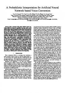
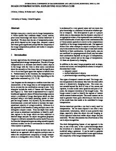
being both aj and bj signed 7 bit integers. In this way, depending on how activation functions are actually computed, floating point stuff is partially or even entirely replaced by very fast and highly parallelizable shift & add operations. 4.3) Experimental Results To make things more visual, we considered it worthwhile to summare the overall performance achieved by the network on the test set by reconstructing binary images from the predicted values of the 64 KL coefficients and computing the percentage of wrong bits.
a)
b)
c)
d) Fig. 1
11
e)
f)
g)
Percentage of Wrong Bits (Test Set)
In Fig. 1 different versions of three patterns extracted from the test set are shown only to exemplify some typical outcomes; the ensuing error measures are taken onto the whole test set. From left to right we have: a) 32 by 20 scaled binary images: the FFN input patterns; b) 32 by 32 binary images: the same patterns immediately before KL expansion; c) What results from the reconstruction through the principal 64 "true" KL coefficients. Such images are in fact those which we have to take as a reference when computing the amount of wrong bits, because quantization in output space is only an artifice we inserted for our convenience; d) Same as c) once KL coefficients are quantized as described before: ⇒ 3.01% of wrong bits; e) Same as d), but now the values provided by the full-fledged FFN are used for reconstruction: ⇒ 5.73% of wrong bits; f) Same as e) once weights are quantized according to (8): ⇒ 5.77% of wrong bits; g) Same as f), but now floating point stuff is totally removed by representing the activation functions of hidden neurons on only 2 bits and those of output neurons on 3 levels alone, so that (4) becomes a sequence of {set to zero | pass-through | shift left} operations followed by an increment: ⇒ 6.46% of wrong bits.
Least Squares Thermo
8 7
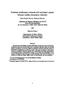
6.49
5
5.77
5.73
6 5.01
6.08
6.46
5.07
4 f/f/f
q/f/f
q/4/f
q/4/3
Resolution of Weights/Hidden Neurons/Output Neurons [f -> floating point; q -> quantized according to (8)] [4 -> 4 Levels; 3 -> 3 Levels]
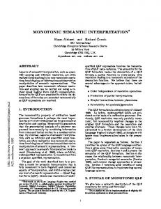
Fig. 2 To compare thermometric recursion with the traditional least squares approach we trained a fully connected 640-82-64 FFN on the same patterns without performing any quantization on the target values. The higher number of hidden units makes the total amount of weights nearly equal to that of the previous network. The histogram in Fig. 2 shows the overall performance achieved by both methods on the test set under the very same conditions, identified by the labels immediately underneath the horizontal axis. Results are in good agreement with what could have been expected in advance. As far as floating point resolution is used on both memory and computing elements, the availability of the "true" KL coefficients makes the least squares-based network superior. In both cases overall performances are loosely affected by weight quantization. Once the activation functions of the hidden neurons are represented on 2 bits then the robustness implied in the
12
distributed nature of the recursive thermometric code prevails. Subsequent quantization of the outputs on 3 levels prevents any meaningful comparison. We now turn to consider the role the uncertainty as given by (5) can play in function estimation problems. To illustrate this point, and for the sake of simplicity, let us take the prediction of the first KL coefficient out of context. Since the chosen number of levels is obviously related with the desired accuracy, it is reasonable to assert that the FFN fails to give the correct response whenever the deviation of the estimate from the true value is larger than the quantization step. Information about uncertainty can then be used to signal if a failure event is likely to occur. By imposing different acceptance thresholds on Var(z), one obtains "Error versus Rejection" curves like the one shown in Fig. 3, that has been produced by the full-fledged version of the same FFN we used before. Here the reference line indicates the expected percentage of failure events in case patterns are rejected in a random fashion. Not surprisingly, the maximum gain occurs when the acceptance threshold for [Var(z)]1/2 is set to about half the quantization step: the limit beyond which the quality of the estimate begins to become questionable. 1.4 Thermo f/f/f Reference
1.2 Error% (Test Set)
1 0.8 0.6 0.4 0.2 0 0
10
20
30
40 50 60 Rejection% (Test Set)
70
80
90
100
Fig. 3
5) Conclusions Today well established links with advanced statistical methods exist that allow a formally correct approach to many important aspects of neural network design. On the other hand, some of the basic principles peculiar to the connectionist paradigm are of great value and should not be altered beyond a certain extent. We showed how standard feed-forward networks can be applied without any theoretical compromise to a wide application domain: that is, the supervised estimation of discrete random variables whose values can be put in a one-to-one ordered correspondence with a finite subset of the natural numbers. To prove the effectiveness of the proposed method, we successfully embedded into a single network a complex pre-processing algorithm that was originally developed by the U.S. National Institute of Standards and Technology for optical character recognition purposes. Full exploitation of all the available prior knowledge made the network extremely robust against the very severe limitations we imposed on the processing units, thus enhancing the advantages offered by a hardware implementation.
6) References 13
[BRI89] Bridle JS. Probabilistic Interpretation of Feedforward Classification Network Outputs, with Relationships to Statistical Pattern Recognition. In: Fogelman-Soulié F, Hérault J (eds), Neurocomputing − Algorithms, Architectures and Applications. NATO ASI Series F68, Springer-Verlag, Berlin (D), 1989, pp 227-236 [COS95] Costa M, Filippi E, Pasero E. Neural Network Ensembles: a Bayesian Standpoint. In: Proc VII Italian Workshop on Neural Networks (WIRN VIETRI '95). Vietri sul Mare − Salerno (I), 1995, pp 39-57 [DEN91] Denker JS, leCun Y. Transforming Neural-Net Output Levels to Probability Distributions. In: Lippmann RP, Moody JE, Touretzky DS (eds), Advances in Neural Information Processing Systems 3. Morgan Kauffmann Publishers, San Mateo (CA), 1991, pp 853-859 [FAB96] Fabbrizio V, Raynal F, Mariaud X, Kramer A, Colli G. Low Power, Low Voltage Conductance-mode CMOS Analog Neuron. In: Proc V International Conference on Microelectronics for Neural Networks and Fuzzy Systems (MicroNeuro '96). Lausanne (CH), 1996, pp 111-115 [FUK72] Fukunaga K. Introduction to Statistical Pattern Recognition. Academic Press, New York, 1972 [GAR92] Garris MD, Wilkinson RA. Handwritten Segmented Characters Database. Tech Rep Special Database 3. National Institute od Standards and Technology, 1992 [GAR94] Garris MD, Blue JL, Candela GT, Dimmick DL, Geist J, Grother PJ, Janet SA, Wilson CL. NIST Form-Based Handprint Recognition System. Tech Rep NISTIR 5469. National Institute of Standards and Technology, 1994 [SPE90] Specht DF. Probabilistic Neural Networks. Neural Networks 1990; 3(1): 109-118 [VIT89] Vittoz E. Analog VLSI Implementation of Neural Networks. In: Proc Journées d'Électronique 1989 − Réseaux de Neurones Artificiels. Lausanne (CH), 1989, pp 223-250 [VOG88] Vogl TP, Mangis JK, Rigler AK, Zink WT, Alkon DL. Accelerating the Convergence of the Back-Propagation Method. Biol Cybern 1988; 59: 257-263
14