Probabilistic Location-Dependent Queries at Different Location Granularities Carlos Bobeda,b , Jorge Bernada,b , Sergio Ilarria,b , Eduardo Menaa,b a Dept.
of Computer Science & Systems Engineering University of Zaragoza, Spain b Aragon Institute of Engineering Research (I3A), Spain
Abstract Approaches for the processing of location-dependent queries usually assume that the location data are expressed precisely, usually using GPS locations. However, this is unrealistic because positioning methods do not have a perfect accuracy (e.g., the positioning approach used in cellular networks handles only the cell where mobile users are located). Besides, users may need to express queries based on concepts of locations other than traditional GPS locations, which we call location granules. In this paper, we focus on location granule-based query processing (i.e., processing of queries with location granules) in situations where the location data available is imprecise, which we have called probabilistic location-dependent queries. For that purpose, we exploit the concept of uncertainty location granule, which represents the location uncertainty of an object. In particular, we tackle the problem of processing probabilistic inside (range) constraints. We analyze in detail how those constraints can be processed, taking into account both the existence of location uncertainty affecting the relevant objects and the location granularity specified. An extensive experimental evaluation shows the feasibility of the proposed probabilistic query processing approach and analyzes the advantages of using index structures to speed up the query processing. Keywords: Location-Dependent Queries, Uncertainty Management, Probabilistic Range Queries, Mobile Computing 1. Introduction
5
Location-dependent queries are queries whose answers depend on the location of certain moving objects [1]. They are a key building block for the development of Location-Based Services (LBSs) [2, 3], which offer value-added data by considering the locations of the mobile users to determine the data that may be relevant. When processing location-dependent queries, GPS locations are
Email addresses:
[email protected] (Carlos Bobed),
[email protected] (Jorge Bernad),
[email protected] (Sergio Ilarri),
[email protected] (Eduardo Mena)
Preprint submitted to Pervasive and Mobile Computing
November 21, 2016
10
15
20
25
30
35
40
45
usually assumed (e.g., [1, 4, 5, 6, 7, 8, 9]). However, users usually think in terms of places instead of coordinates (i.e., they think in terms of higher-level location granularities), being precise locations frequently irrelevant for them. For example, an app for tourists could allow them to look up where they are (e.g, address, district name, etc.), and to look for interesting points (e.g., museums, stadiums, etc.) by choosing their own terms (e.g., show me museums in downtown) without having the user to define the specific boundaries of the relevant areas (the app would know better than the user which the downtown area is). As another example, if a user is travelling by subway, he/she may want to know the name of the next station, along with information about the district where it is located. So, when expressing queries and retrieving their results, it is important to manage the location granularity required by the user. To be able to provide different views on the raw GPS locations, extending them with semantics, we introduced the concept of location granule in [10, 11] as a set of geographical areas which identify a set of GPS locations under a common name (e.g., in the example of the subway the area of each station and district would be a different location granule, and an inclusion relationship would relate those types of granules). This concept of location granule is similar to the notion of place [12, 13] or spatial granule [14] proposed in the literature. In this way, location granules are geographical areas which represent locations with meaningful semantics for the user, providing a more coarse-grained location representation than GPS 1 (e.g., cities, regions, countries, roads, buildings, rooms in a building, etc.). To handle them within location-dependent queries, we presented a query processing approach in [11], and extended it with two complementary models to represent location granules semantically in [10] and [15]. However, these previous proposals assume that the precise GPS locations of the moving objects are available, even though if later those locations are converted into location granules. This is an unrealistic assumption because of several reasons: • Positioning methods are subject to imprecision [16] due to different reasons. On the one hand, we can find that the positioning method might have an inherent precision error and provide an area where the object might be [17, 18], or directly have a granularity coarser than required (i.e., cell-based location methods [19]). On the other hand, in the context of mobile objects, we could find that the location data is not updated as frequently as we would like, and therefore we have to assume some imprecision in the location of a moving object (e.g., providing an estimation taking into account its velocity and direction [20]). • Locations can also be deliberately obfuscated to enhance privacy using different methods [21, 22]. For example, if the location method can only retrieve which street the user is in (e.g., due to his/her preferences), in1 Note that this does not imply that GPS locations are neglected. On the contrary, GPS locations can be translated into (and be used jointly with) meaningful area definitions.
2
50
55
60
65
70
75
80
85
90
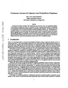
stead of his/her GPS location, querying for nearby objects must take into account that the user might be in any particular position within that street. Whenever there is uncertainty in the location of the objects, we cannot provide a completely precise answer, and thus, proposing a query processing approach that does not rely on the location precision assumption is needed. In this paper, we focus on the processing of probabilistic location-dependent queries with location granules, that is, queries where location granules must be used taking into account that the location information available about the objects in the scenario is imprecise. Such location uncertainty in every of aforementioned imprecision sources can be modeled using an uncertainty area whose shape and probability distribution depends on the imprecision source (e.g., we can calculate it out of the position and velocity as in mobile object databases [23], or be given by a mathematical model of the used location method). Thus, to model such imprecision sources, our proposal is based on the definition of uncertainty location granule, which represents the location of an object through a probability density function that provides the probability that the object is in each point of the area of the granule. More specifically, we tackle inside constraints, which retrieve the objects of a certain class (target objects) located within a given spatial range around a specified moving object (reference object). For example, let us imagine a user that is looking for friends that are in the whereabouts, using an app for such a purpose. This app could allow users to specify the area of search at different granularities: street, neighborhood, city, etc. In our case, let us assume that s/he wants to retrieve friends located on the same street where s/he is. Independently of the technology used to locate the user, there always exists a certain location error; when precise localization methods (such as GPS, with an imprecision of just a few meters) are not available (e.g., indoor locations, tunnels, turned-off GPS devices, etc. ), using other technologies such as WiFi triangulation or power maps, cell phone IDs, etc., lead to a significant uncertainty regarding the user’s location. Thus, due to the imprecision, the user might be on different streets with different probabilities. Besides, his/her friends might also have imprecise localization methods, or just not have updated their locations in the app (or even some of them have obfuscated their location by only showing his/her street, neighborhood, city, etc., where s/he is currently located), which also would influence the probability of them being on the same street as the user is. In summary, in order to provide an answer in mobile computing environments, we cannot avoid dealing with uncertainty, as assuming precise and perfectly updated locations of objects in the scenario is unrealistic. In Figure 1, the imprecise location of a user can be seen (the user can be in any place of the gray circle), so the user could be on street A, B, or C with different probabilities: It is clear that (if we assume a uniform probability distribution) the user will be with high probability on street A or B, and will be on street C with a very low probability. The imprecise location of his/her 3
95
nearby friends are the green circles, and so friends that would probably be on streets A or B (friend3, friend4, and friend5 ) would be much more likely to be on the same street as our user. friend1 friend2 street C friend5
street A friend3
str e friend4 et B
user
Figure 1: Retrieving friends on the user street when locations are imprecise. The uncertain locations are represented by circles (in gray, the user; and, the greener, the more probable that such a friend is on the user street).
100
105
110
115
120
As we will see, the calculation of the objects that hold such constraints requires solving some integrals numerically, which has an important impact on the efficiency of the query processing. Thus, we adopt an indexed approach to filter out as many objects as possible in the early stages of the query processing. A preliminary work about probabilistic granule-based queries was presented in [24]; here, we improve and extend that seminal proposal in a number of ways, including the introduction and analysis of uncertainty location granules for uniform and normal probabilistic distributions, and an extensive experimental evaluation. The uniform pdf is applied when there is no information about the imprecision of the location of an object. In that case, we consider the worst case: The object can be in any place of an uncertainty area with equal probability [23]. Another usual assumption is to consider that the imprecision of the location follows a bivariate normal distribution [25, 26]. Thus, in this work, we focus on inside queries and provide a systematic and detailed study of such type of queries in the case of both uniform and normal uncertainty distributions. The main contributions of this paper are: • We define new types of location-based inside queries that involve location granules with and without uncertainty. • We analyze those queries considering that any probability density function is used to model the location uncertainty, and particular solutions are given when the underlying probability density function is the uniform or normal distribution. • We propose a spatial granule-based index approach to solve inside constraints with uncertainty and location granules. We have tested this indexing approach with an extensive experimental evaluation, where the efficiency of the described method for both the uniform and normal distributions can be appreciated. 4
125
130
The structure of the rest of this paper is as follows. In Section 2, we present an overview of the proposed model of location granules, extending their definition to incorporate uncertainty, and we describe an indexing approach to efficiently process queries with location granules. In Section 3, we formally define the problems that we tackle in this paper focusing on probabilistic inside queries, and explain our approach to tag objects with their probabilities of being part of the answer to the query. In Section 4, we present an experimental evaluation that shows that the probabilistic granule-based location-dependent queries studied in this paper can be supported efficiently. In Section 5, we present some related work. Finally, in Section 6, we draw some conclusions and point out some ideas for future work. 2. Location Granules and Uncertainty
135
In this section, first, we explain the types of entities that we use to model environments without uncertainty, introduced in [11]. Then, we detail how we extend this model to include uncertainty. Finally, we propose an indexing approach for this model. 2.1. Model without Uncertainty: Location Granules
140
145
150
155
160
165
In order to model a location-aware scenario, we proposed in [11] a model based on the notion of location granule, which, intuitively, can be defined as a set of one or more geographical areas which represent a coarser location under a common name. Such a model, which did not include support to deal with uncertainty, was based on three main elements [11]: • Objects (O): An object represents an entity located in a position of the plane. It is characterized by an internal (system-managed) identifier, a name, a GPS location (xo , yo ), a class, and probably other attributes specific to its class. For example, objects can be used to state that a vehicle is at a certain (x1 , y1 ) location and it is an ambulance (its class type is an ambulance), while another vehicle is at (x2 , y2 ) and it is a fire truck. • Location Granules (LG): A location granule (or simply, a granule) refers to one or more geographic areas or polygons which identify a set of GPS locations under a common name. Specifically, a location granule G is characterized by a triple hid, name, GA i, where id is an internal (systemmanaged) identifier, name is the name of the granule, and GA is an area of the plane, i.e., GA ⊆ R2 . Location granules can be used to model areas with different semantics and granularities. For example, we can model areas such as countries (e.g., USA, Spain, etc.), states (e.g., California, Washington, etc.), or places (e.g., Central Park, the Grand Canyon, a certain mall, the Union Station in Washington D.C., etc.). • Granule Maps (GM): A granule map is a set of location granules. More precisely, a granule map M is characterized by a tuple hid, name, SM i, where id is an internal (system-managed) identifier, name is the name of the granule map, and SM is a set of granules, SM = {G1 , . . . , Gn }. For instance, with granule maps, we can express the map of the states of 5
USA, where each state is a location granule which belongs to the granule map, or the map of USA counties, depending on the location granularity required. 170
175
180
185
Along these elements, we also defined a set of operations: inGr is a function that, given a location granule G and an object o, returns a boolean value indicating whether the location of the object, (xo , yo ), belongs to the area GA of G; dist computes the distance between an object’s location and a granule; and distBtwGrs computes the distance between two granules. Different types of distance can be considered: the limits-distance (the minimum distance to the boundaries of the areas composing the granule), the centroid-distance (the distance to the centroids of the granules), and the outsideLimitsBased-distance (a variation of the limits-distance in which all the inner points of the granule are considered to be at zero distance). Without loss of generality, by default we assume the limits-distance. The last two defined operators deal with granule maps: getGrs is a function that, given a granule map M and an object o, retrieves all the granules in SM where the location of o belongs, that is, the set {Gi ∈ SM | (xo , yo ) ∈ Gi }; getN earGr returns the granule Gi , in a granule map M , that is the nearest to the location of an object. However, in this proposed model, no special provisions were made to consider location uncertainty, which could be introduced by many causes. Thus, in the following, we propose an extension to our model to seamlessly integrate location uncertainty. 2.2. Model with Uncertainty: Uncertainty Location Granules
190
195
200
205
210
To deal with imprecise locations and probabilistic queries in our model, we extend the basic model by introducing the notion of uncertainty location granule. Definition 1. An Uncertainty Location Granule (ULG), O, is a tuple O =hid, U GO , pdfO i composed by: an internal (system-managed) identifier id; U GO is an area or a discrete set of points contained in R2 , and we will say that U GO is the uncertainty area of O; and pdfO is a probability density function (pdf ) such R that U GO pdfO = 1; if U GO is a discrete set of points, pdfO is a probability P mass function, and so x∈U GO pdfO (x) = 1. An element o ∈ U GO is said to be an instance of the uncertainty location granule O. With uncertainty location granules, we can model an imprecise location. For example, given the GPS location of an object, we can consider that such an object is inside a circle centered at such GPS location and whose radius depends on the precision (maximum possible error). In this case, the uncertainty location granule could be hid, U GO , pdfO i, where U GO is a disk and pdfO is a truncated Gaussian pdf over the disk. We can also model the anonymization of a user’s position [27]: the uncertainty area U GO could be a rectangle (or some other polygon) and pdfO would be the uniform pdf over U GO , which means that the object can be with the same probability in any location within the area of the uncertainty location granule. The set of operators described in Section 2.1 is also enriched with three new operators that relate uncertainty location granules and location granules: 6
• inGrP rob(O, G) is a function that returns the probability that the object represented by the uncertainty location granule O is Rinside a granule G. This probability is calculated by inGrP rob(O, G) = U GO ∩GA pdfO . We will also denote this probability by P (O ∈ G). 215
220
225
• distP rob(O, G), where O is an uncertainty location granule and G is a G location granule, returns a pdf for the random variable DO : U GO → R G such that for any instance o ∈ U GO , DO (o) = dist(o, G). It is used to calculate the probability that the object represented by the uncertainty location granule O is at distance less than or equal to R from the location RR G granule G, that is, P (DO ≤ R) = 0 distP rob(G, O)(x)dx. • distP rob(O1 , O2 ), where O1 and O2 are uncertainty location granules, O2 returns a pdf for the random variable DO : U GO1 × U GO2 → R, where 1 O2 (o , o ) = dist(o , o ). The returned pdf is used to calculate the DO 1 2 1 2 1 probability that the distance between O1 and O2 is less or equal to R, RR O2 P (DO ≤ R) = 0 distP rob(O1 , O2 )(x)dx. 1 Datatype Object (OB) Location Granule (LG)
Tuple format hid, name, loc, class, otherAttri hid, name, GA i
Granule Map (GM)
hid, name, SM i
Uncertainty Location Granule (ULG)
hid, U LGt , density functioni
Operators dist: OB x OB → Real inGr: LG x OB → Boolean dist: LG x OB → Real distBtwGrs: LG x LG → Real getGrs: GM x OB → P(LG) getNearGr: GM x OB→ LG inGrProb: ULG x LG → Real distProb: ULG x LG → PDF distProb: ULG x ULG → PDF
Table 1: Basic probabilistic data model: data types and main operators for location granules and uncertainty location granules.
230
A complete summary of the data types and operators can be seen in Table 1. Let us note that the introduction of imprecise locations implies calculating some integrals to process the queries, as it will be explained in Section 3.3. Since the computation of these integrals could have a direct impact on the performance (even when uniform pdfs are assumed), we should compute as few integrals as possible. For this reason, we introduce the following a structure to index the uncertainty location granules and the granules in the granule maps. 2.3. Grouping and Indexing Location Granules
235
240
In order to process efficiently granule-based inside constraints, we propose to use two independent spatial indexes to manage separately location granule maps and objects (with or without uncertainty). The rationale behind this two-index schema is to take into account the volatility of the information being indexed: The geographical data that define the different location granules where the objects are located are less prone to change than the precise geographic locations of the moving objects in the scenario. 7
245
250
Moreover, our approach is oriented to quickly filter those elements which are clearly not relevant for the query that is being processed. Thus, no probability tagging is performed at this level, but only filtering out those elements whose probability of being part of the answer to a query posed to the index is zero. Thus, we propose to use a Spatial Granule-Based Index (SGBI), a data structure which is formed by a tuple hGM I, OIi, where: • GMI (Granule Map Index) is a hash table which stores several spatial indexes, each of which indexes a different granule map (and, thus, a different layer/view on the scenario). • OI (Object Index) is a spatial index which stores the different objects in the scenario taking into account their uncertainty areas. Apart from the methods to load and index granule maps and objects, the SGBI provides us with three main operators:
255
• getGranules(GranuleMapName, GPS) returns the set of location granules of a given granularity that might contain the given GPS location using the GMI. • getGranules(GranuleMapName, Area) returns the set of location granules of a given granularity that might intersect the given area using the GMI.
260
265
270
• getObjects(Area) returns the set of objects which might be within the given area, using the OI. Note that we do not make any assumption about either the underlying indexing techniques (location granules and objects ones), or the pdfs used to model the uncertainty in the locations. In our current implementation, we have used PR-Trees [28] for both indexes in the schema. Thus, we index both location granules and objects with their uncertainty pdfs according to their Minimum Bounding Rectangles (MBRs). As we will see in Section 4, this filter is efficient enough to process such constraints in an efficient and scalable manner. However, we are aware that we can leverage more spatial and pdfs’ information to improve our approach, and we will explore it in the future. In the following section, we will present the different probabilistic location constraints we deal with in this paper. 3. Probabilistic Granule-Based Inside Queries
275
In this section, we tackle the processing of probabilistic granule-based inside queries. First, we briefly present the change of semantics of inside queries when location granules come into scene. Then, we formally define the different query constraints that we consider in this paper. Finally, we describe how such constraints are processed. 3.1. Preliminaries: Granule-Based Inside Queries
280
The use of location granules in a location-dependent query can affect the semantics and the way the query is processed. As an example, let us imagine a
8
285
290
295
vehicle fleet management system monitoring some trucks over France2 to control and plan their routes. Let us suppose that a truck is broken down and it needs to be repaired. Due to insurance restrictions, the truck can only be serviced in garages which are within the same region, or, at the furthest in the nearest departments of adjacent regions. Thus, in our system, we would like to know which garages (we will call them target objects, as they are the objects that must be retrieved) are not farther than r kilometers from the region (FrRegion) where the broken truck is (we will call it the reference object, as it is used as a reference for the query constraint). Instead of expressing the query using raw GPS coordinates (which would require the final user of our system to know the exact GPS coordinates of all the regions and departments, as well as to define a complex query to describe the appropriate distances between elements in the query), our system allows to use the appropriate location granularities for the query, handling appropriately the semantics of distances at different granularities (i.e., the distance definition might change when different granularities are used). Using the SQL-like query language presented in [11], this constraint would be expressed as follows: inside(R, gr(“FrRegions”, refObj), gr(“FrDepartments”, tgt))
300
305
310
315
320
where R is the radius of the inside constraint, refObj represents the identifier of a reference object, tgt indicates the class of the target objects (we will call it the target class, which is garage in the previous example), and gr is the getGrs operator that returns the granules an object is within based on the granularity specified. Notice that interesting objects (certain garages, and their GPS location, fulfilling some geographic constraints) will be obtained taking as basis the GPS location of the reference object (the damaged truck) only after dealing with location granules: on the one hand, the region of the damaged truck, which is used 1) to obtain garages inside it, and 2) to obtain adjacent departments from other regions where garages can be found; and, on the other hand, each adjacent department, which is used to obtain garages inside such an area. The query is not as simple as asking for target objects within a given distance from the reference object. On the contrary, our system also supports specifying constraints about distance among objects and areas, or among areas and other areas. Thus, the way this constraint is processed is illustrated in Figure 2. The first step is to obtain the location of the reference object (see Figure 2.a), which represents in this case the center of the inside constraint. Next, the location granule in which the object is located is obtained according to the granule map specified for the reference object in the constraint (in the example, the granule map is the set of French regions and the granule obtained is the Center region of France), and the boundary of such a location granule is extended in 2 We are using in these examples administrative divisions (i.e., regions) and their subdivisions (i.e., departments) traditionally considered in France. Thus, in France, each region is composed by one or more departments.
9
325
all directions according to the distance specified in the inside constraint (see Figure 2.b), which is called buffering in the context of Geographic Information Systems [29]. Finally, the target objects that lie in the granules of the granule map specified for the target objects (in the previous example, the granule map of departments) that intersect the previously calculated area are retrieved (see Figure 2.c).
Figure 2: Processing an inside constraint with region granularity for the reference object and department granularity for the target objects: a) Detect the reference object (red point) in the Center region; b) Obtain the granule the reference object lies within, and extend its area by the inside radius (extended area, blue line); c) Retrieve target objects which lie within granules that intersect that extended area (orange points).
330
The impact of using different granularities on the location-dependent constraint can be easily observed if we move to the example in Figure 3, where we are interested in retrieving the garages that are inside regions which are not farther than R kilometers from the department where our truck is located. Using the same syntax as in the above example, this constraint would be expressed as follows: inside(R, gr(“FrDepartments”, refObj), gr(“FrRegions”, tgt))
335
340
345
Specifically, in Figure 3.a, the inside constraint is expressed using the granule map of departments of France for the reference object and the granule map of regions of France for the target objects (as expressed in the previous constraint), whereas in Figure 3.b the opposite approach is taken (departments for the target objects and regions for the reference object). Even though the objects in the scenario are in the same locations, we can notice that the answer to the query would be quite different. Let us note that the above-explained location-dependent queries use granule maps for the reference and the target objects. It is also possible to define queries with a granule map only for the reference object (e.g., return those garages that are not farther than R kilometers from the department a certain truck is in), or only for the target objects (e.g., return those garages that are inside departments which are not farther than R kilometers from the location of a given truck).
10
Figure 3: Inside queries with different semantics depending on the granularity used: a) Retrieved objects (orange points) when department granularity is specified for the reference object and region granularity is specified for the target objects; b) Retrieved objects (orange points) when region granularity is specified for the reference object and department granularity is specified for the target objects.
350
In the following section, we will modify the definition of these types of queries (presented initially in [11]) to consider uncertainty. For example, if we cannot be sure about the precise locations of the objects, and it is only known that each of them is inside a particular area with some probability, how can these queries be processed? 3.2. Problem Statement
355
360
365
In a scenario with imprecise locations involving uncertainty location granules, we can find three different kinds of probabilistic granule-based inside constraints: when a granule map is specified for the reference object (Definition 2); when a granule map is specified for the target objects (Definition 3); and, finally, when granule maps (a single granule map or two different granule maps) are specified for both the reference object and the target objects (Definition 4). As far as we know, these are new types of queries, not defined and studied previously in the literature. Definition 2. Let D = {O1 , . . . , On } be a set of uncertainty location granules (target objects), Or be an uncertainty location granule (reference object), and Mr = {G1 , . . . , Gn } be a granule map. A probabilistic granule-based inside query with a granule map for the reference object retrieves the uncertainty location granules of D that are no farther than R from the granules Gj where the reference object Or might be located, with a probability greater or equal than p: q(D, Or , Mr , R, p) = {Oi ∈ D |
n X
G
P (Or ∈ Gj )P (DO j ≤ R) ≥ p} i
j=1
11
370
Definition 3. Let D = {O1 , . . . , On } be a set of uncertainty location granules (target objects), Or an uncertainty location granule (reference object), and Mt = {H1 , . . . , Hm } a granule map. A probabilistic granule-based inside query with a granule map for the target objects retrieves the uncertainty location granules of D with a probability greater or equal than p to be in a granule Hj ∈ Mt that is not farther than R from the reference object Or : q(D, Mt , Or , R, p) = {Oi ∈ D |
m X
H
P (Oi ∈ Hj )P (DOrj ≤ R) ≥ p}
j=1
375
380
Definition 4. Let D = {O1 , . . . , On } be a set of uncertainty location granules (target objects), Or an uncertainty location granule (reference object), and Mr = {G1 , . . . , Gn } and Mt = {H1 , . . . , Hm } granule maps. A probabilistic granulebased inside query with granule maps for target and reference objects retrieves the uncertainty location granules of D with a probability greater or equal than p to be in a granule Hl ∈ Mt that is not farther than R from a granule Gk ∈ Mr where the reference object Or might be located. That is, if we denote by dkl = distBtwGrs(Gk , Hl ), then we have: q(D, Mt , Or , Mr R, p) = {Oi ∈ D |
n X m X
P (Or ∈ Gk )P (Oi ∈ Hl )H(R − dkl ) ≥ p}
k=1 l=1
where H(x) is the Heaviside function: H(x) = 1 if x ≥ 0, and H(x) = 0 otherwise.
385
390
395
Note how, regarding the probability threshold provided as an input to the query, these definitions support must and may semantics [30]: must semantics, when the query is specified to retrieve only the objects that satisfy the query constraint for sure (i.e., with 100% probability); and may semantics, when the query is specified to retrieve any object that may satisfy the query constraint, but with no guarantees (i.e., specifying a probability threshold lower than 100% that the retrieved object must accomplish). It is not expected that the user will manually set the probability threshold specifically for each query; instead, the application used by the user could manage internally several predefined thresholds (e.g., possible 0%, likely 60%, high 80%, very high 90%, sure 100%) and use them dynamically for the queries according to the learnt user preferences. In the following section, we analyze each of the three types of probabilistic granule-based inside constraints discussed, and illustrate the different steps that their processing requires. 3.3. Processing the Constraints In this section, we analyze in detail how the different query constraints are processed3 . For simplicity of exposition, we model the uncertainty with 3 The algorithms for processing the different types of queries presented in this section are shown in Appendix A of the additional material, which can also be found at http://sid.cps. unizar.es/projects/ProbabilisticGranules
12
400
a continuous probability density function for all the objects in all the scenarios. The discussion for a discrete probability mass function would be analogous, substituting the different integrals by the appropriate summations. Moreover, for better readability, we present in Table 2 a summary of the notations used throughout this section. G EA(G, R) Oi =hid, U Gi , pdfi i P (O ∈ G) G DO distP rob(O, G) G ≤ R) P (DO
N (µ; Σ)
Location granule. Extended area of a location granule, i.e., the area obtained by extending G a distance R in all the directions. Uncertainty granule with associated uncertainty area U Gi and probability density function pdfi . Probability that the uncertainty granule O is in the location granule G. Random variable that for any instance o ∈ U GO returns dist(o, G). G. Probability density function for DO Probability that the distance between G and O is less or equal to R, i.e., the cumulative distribution function of distP rob(G, O). Bivariate normal distribution with mean vector µ and covariance √ R T −1 1 matrix Σ: N (µ; Σ) = 1/(2π Σ) e− 2 ((x−µ) Σ (x−µ))
Table 2: Summary of the basic notations used in Section 3.3.
405
410
415
420
3.3.1. Probabilistic Inside Constraints with Granule Map for the Reference Object Firstly, we deal with the queries defined in Definition 2, i.e., retrieve target objects which are not farther than R from the location granule where a reference object is; e.g., “Which ambulances (target objects) are not farther than R from the region (granule map for the reference object) where an accident (reference object) happened”. If we are dealing with precise locations, in this case, we must first discover in which granule the reference object is in, and then retrieve the target objects that are no farther than R from such a granule4 . However, if a location granule map has been specified for the reference object and the location of the reference object is uncertain, we might have several granules where the accident could have happened with different probabilities. So, we have to calculate the probability for each of the location granules to be the actual one where the reference object is in, in order to obtain the actual probability of each target object to be within an R distance. To do so, we propose to handle the uncertain locations as uncertainty location granules (which are not granules existing in the granule maps used, but dynamically obtained from the object’s location and its location imprecision model). Thus, we have to obtain the granules which intersect the uncertainty location granule that represents the location of the reference object, and cal4 For the sake of simplicity, we assume in the explanation that an object with a precise location lies only within a single location granule. However, our approach supports overlapping location granules by performing the union of their areas.
13
425
culate their probabilities by integrating the pdf associated to the uncertainty location granule on each of the different intersecting areas. Intuitively, in Figure 4, we can see the different steps of processing an inside constraint specifying a granule map for the reference object: R G1
UGt O O t t
UGr Or G1
G1 G2
Ot
UGr
R
UGt UGr
Or
Or
G1 G2
UGt O O t
G2
t
UGr
UGt Ot
R
Or G2 R
a)
b)
c)
Figure 4: Inside constraint processing with uncertain locations and the specification of a granule map for the reference object: a) Find granules where Or might be (G1 , G2 ) using its uncertainty location granule (circle U Gr ); b) Find target objects Ot (using their U Gt ) that might be in the extended areas EA(Gi , R) of such granules (the gray areas define their probabilities); c) Aggregate the final probabilities for each Ot .
430
435
440
445
• First, we obtain the granules in the granule map where the reference object Or might be (G1 and G2 in Figure 4.a). • Then, as each of these granules contributes to the probability of Ot being part of the answer, we have to calculate the probability of Or being at each of the granules (intersections of U Gr with G1 and G2 in Figure 4.b). For each of the granules which has a non-zero probability, we have to calculate the probability of Ot being at less than an R distance from them (intersections of the extended areas EA(G1 , R) and EA(G2 , R) with U Gt in Figure 4.b). • Finally, we have to weight and aggregate the different contributions to calculate the actual probability of Ot being part of the answer set (Figure 4.c). Formally, let Or and Ot be a reference and a target object with associated uncertainty location granules hidr , U Gr , pdfr i and hidt , U Gt , pdft i, respectively, and Mr = {G1 , . . . , Gn } be a granule map for the reference object. We denote by EA(Gi , R) the extended area of a granule Gi ∈ Mr by the radius R (the distance threshold for the inside constraint), i.e., EA(Gi , R) = Gi + B(0, R), where B(0, R) is a ball centered at the origin and radius R, and + is the Minkowski 14
450
sum (buffering operation). The probability that the object Ot is in the answer set (AS) is the sum, for each possible granule Gi , of the probability that the reference object is in the granule Gi multiplied by the probability that the target object is in the extended area of the granule Gi , that is: X
P (Ot ∈ AS) =
P (Or ∈ Gi )P (Ot ∈ EA(Gi , R))
Gi ∈Mr
Therefore, using the probability density functions pdfr and pdft , we have that: Z
X Z
P (Ot ∈ AS) =
Gi ∩U Gr
Gi ∈Mr
pdft
pdfr
(1a)
EA(Gi ,R)∩U Gt
Computation with the Uniform Distribution If we consider the case that we have a uniform pdf, then the formula can be simplified to calculate areas: P (Ot ∈ AS) =
X Area(Gi ∩ U Gr ) Area(EA(Gi , R) ∩ U Gt ) Area(U Gr ) Area(U Gt ) G ∈M i
(1b)
r
Computation with the Normal Distribution For the normal distribution, we have: P (Ot ∈ AS) =
X Z Gi ∈Mr
455
Z N (µr ; Σr )
Gi
N (µt ; Σt )
(1c)
EA(Gi ,R)
where N (µ; Σ) is a bivariate normal distribution with mean µ and covariance matrix Σ. 3.3.2. Probabilistic Inside Constraints with Granule Map for the Target Objects
460
465
470
Now, we move onto the queries defined in Definition 3, i.e., retrieve target objects that are within location granules which are not farther than R from the location of the reference object; e.g., “Which ambulances (target objects) are situated in regions (granule map for target objects) that are not farther than R from a car accident (reference object)”. It is similar to the previous case, but now the target objects Ot are the ones that have associated a list of potential location granules along with their probabilities. Looking at Figure 5, intuitively: • First, we identify the granules that are at a distance less than R from Or (H1 and H2 in Figure 5.a) where, for simplicity and without loss of generality, we are assuming that H1 and H2 are granules with the same shape than the granules G1 and G2 shown in Figure 4). • Then, for each of those granules, we have to calculate its exact probability of being within a distance R from the reference object; in Figure 5.b, the intersections of U Gr with the extended areas of the different granules are all the points where Or can be at less than such a distance. For each of the granules which has a non-zero probability, we have to calculate the probability that Ot is within that granule (intersection of U Gt with H1 and H2 in Figure 5.b). 15
R H1 UGt O O t
R
t
UGr
H1
H1
UGt
Or
UGt
H2
O O t
UGr
H1 UGt
Or
H2 R
Ot
UGr
t
O O r r
H2
O Ot t
UGr
R
Or
H2 R
a)
b)
c)
Figure 5: Inside constraint processing with uncertain locations and the specification of a granule map for the target objects: a) Find all the location granules that might be at distance less than R from Or (H1 , H2 ) using its uncertainty location granule (U Gr ); b) Calculate the probability of each Hi being within an R range, and, for each target object Ot that might lie within Hi , calculate their probability; c) Aggregate the final probabilities for each Ot .
475
• As in the previous constraint, we have to ponder and aggregate the different contributions to calculate the actual probability of Ot being part of the answer set (Figure 5.c). Similarly to what was shown for the previous type of probabilistic granulebased constraint, if we denote by Mt = {H1 , . . . , Hm } the granule map for the target objects, we can calculate the probability that the target object Ot is in the answer set AS by: P (Ot ∈ AS) =
Z
X Z Hi ∈Mt
pdft
pdfr EA(Hi ,R)∩U Gr
(2a)
Hi ∩U Gt
Computation with the Uniform Distribution If we consider uniform pdfs, again the probabilities can be computed by calculating areas: P (Ot ∈ AS) =
X Area(EA(Hi , R) ∩ U Gr ) Area(Hi ∩ U Gt ) Area(U Gr ) Area(U Gt ) G ∈M
(2b)
i
Computation with the Normal Distribution For the normal distribution, we have: Z X Z P (Ot ∈ AS) = N (µr ; Σr ) N (µt ; Σt ) (2c) Hi ∈Mt
EA(Hi ,R)
16
Hi
480
485
3.3.3. Probabilistic Inside Constraints with Granule Map for Both the Reference Object and the Target Objects Finally, we deal with the queries defined in Definition 4, i.e., retrieve target objects that are within location granules which are not farther than R from the location granule where the reference object lies; e.g., “Which fire trucks (target objects) are in regions (granule map for target objects) that are not farther than R from the city (granule map for the reference object) where a car accident (reference object) happened”. We illustrate how to process these constraints with Figure 6: R H1
G1
H1
G1 UGt1
UGt1 UGt2
Ot1 t UGr
UGt2
Ot1 t UGr
Ot2
Ot2 Or
Or H2
H2
G2
G2 R
a)
b)
Figure 6: Inside constraint processing with uncertain locations and the specification of a granule map for both the reference and the target objects: Contributions of the probabilities of Or being inside G1 and G2 (parts a and b in the figure, respectively) to ponder the probabilities of Ot1 and Ot2 of being part of the answer set by affecting the maximum probabilities of the location granules they might lie within (H1 and H2 ).
• First, we obtain the granules in the granule map where the reference object Or might lie (intersection of U Gr with the granules G1 and G2 ). 490
495
• For each of the intersected granules, we have to obtain the granules in the granule map for the target objects that are not farther than R from them. Note that, at this point, we are perfectly sure about the distances between granules (they are not uncertainty location granules) and we can obtain them by buffering the granules Gi and intersecting them. • For each of the previously-obtained granules (granules H1 and H2 in the figure), we have to calculate the probability of Ot being within them (intersection of U Gt with them). • Finally, again, we have to ponder and aggregate each of the contributions. Formally, we denote by Mr = {G1 , . . . , Gn } the granule map for the reference object Or , and by Mt = {H1 , . . . , Hm } the granule map for the target objects. As previously, EA(Gi , R) denotes the extended area of the granule Gi , and hU Gr , pdfr i and hU Gt , pdft i the uncertainty location granules Or and 17
Ot , respectively. If M is a granule map and B is a granule, we use the notaM tion N EB = {H ∈ M | H ∩ B 6= ∅} to denote the granules H in the granule map M that have non-empty intersection with the granule B. We can find the probability that a target object is in the answer set, P (Ot ∈ AS), as follows: P (Ot ∈ AS) =
X
X
P (Or ∈ Gi )P (Ot ∈ Hj )
Gi ∈Mr H ∈N E Mt j G i
In this way, we compute the summation of the probability that the reference object is in a granule Gi of the granule map Mr multiplied by the probability that the target object is in a granule Hj of Mt such that Hj ∩ EA(Gi , R) is not empty. In terms of the density functions, we have: X
P (Ot ∈ AS) =
Z
X
Z pdfr
Gi ∈Mr H ∈N E Mt j G
Gi ∩U Gr
pdft
(3a)
Hj ∩U Gt
i
Computation with the Uniform Distribution As in the previous cases, Equation 3a can be calculated for uniformly distributed pdfs as: P (Ot ∈ AS) =
X
X
Gi ∈M H ∈N E Mt j Gi
Area(Gi ∩ U Gr ) Area(Hj ∩ U Gt ) Area(U Gr ) Area(U Gt )
(3b)
500
Computation with the Normal Distribution For the normal distribution, we have: P (Ot ∈ AS) =
X
Z
X
Z N (µr ; Σr )
Gi ∈Mr H ∈N E Mt j G
Gi
N (µt ; Σt )
(3c)
Hj
i
505
510
For clarity, we include Algorithm 1 to illustrate the details of the processing of this type of queries using the proposed SGBI described in Section 2.3. First, we have to obtain the possible granules where the reference object lies using the SGBI (line 3). For each of those possible candidates (lines 4–20), we calculate the probability that the reference object actually lies within it (line 5). For those granules that contribute to the answer, we calculate their buffering and obtain the granules that might be at a distance less than R from them using the SGBI (lines 7–8). Then, after checking whether they are actually at such distance (line 10), we proceed to obtain the target objects which might lie within each target granule using the SGBI (line 11). For those filtered objects, we calculate their probabilities according to the formulation we have shown and update them to obtain the final probability (lines 13–14). Finally, the set of candidate objects is filtered using the probability threshold (line 22).
18
Algorithm 1 Query processing with granule maps for the ref. and the target objects Require: Regarding the input: SGBI is the spatial index, GM apN ameRef is the granule map to be used for the reference object, GM apN ameT gt is the granule map to be used for the target objects, ref Object is the reference object in the constraint, R is the radius of the inside query, and threshold is the probability that the objects in the answer set must achieve. It also requires geom, an object specialized in performing geometric operations. Ensure: Retrieves the objects that satisfies the constraint with a probability above the given threshold. 1: /* candSet is a table where each object is tagged with its probability */ 2: candSet ← ∅ 3: candRefGranules←SGBI.getGranules(GMapNameRef, refObject.UG.area) 4: for g in candRefGranules do 5: probRefObjectInG ← inGrProb(g, refObject) 6: if probRefObjectInG > 0 then 7: extArea ← geom.buffer(g.area, R) 8: candTgtGranules ← SGBI.getGranules(GMapNameTgt, extArea) 9: for h in candTgtGranules do 10: if geom.intersects(extArea, h.area) then 11: affObjects ← SGBI.getObjects(h.area) 12: for obj in affObjects do 13: probInGranuleH ← inGrProb(h, obj) 14: // update the probability by adding the current value 15: candSet.update(obj, probRefObjectInG * probInGranuleH) 16: end for 17: end if 18: end for 19: end if 20: end for 21: // filter out the objects above the probability threshold 22: candSet.filterOut(threshold) 23: returns candSet
515
4. Experimental Evaluation
520
To validate our proposal in terms of performance and scalability, we have performed an extensive experimental evaluation. In Section 4.1, we first specify the implementation details of our prototype and the experimental settings. Then, we present our experimental results using different sets of granule maps in Sections 4.2 and 4.3. 4.1. Experimental Settings
525
To show the feasibility of our approach, we have developed a prototype that is capable of processing location-based queries with granule-based inside constraints in the presence of location uncertainty. Our prototype has been implemented using Java 1.7 as programming language, and the JTS Topology Suite 1.135 . We have also developed an interactive applet6 to help visualizing the 5 http://sourceforge.net/projects/jts-topo-suite/ 6 http://sid.cps.unizar.es/projects/ProbabilisticGranules/granulesApplet.html. Note that applets are not currently supported by the Chrome browser, so we provide an alternative Java WebStart version available in this webpage.
19
530
535
540
545
550
555
560
565
semantics of the granule-based constraints when uncertainty comes into play. In the following, we detail the specifics for the scenarios and the parameters which are considered in the experiments for the three type of queries described in Section 3.2, as well as the algorithms used to calculate the required integrals. Pdfs considered and integral calculations In the experiments, we have evaluated our approach adopting both the uniform and normal probability distributions as uncertainty models. Indeed, the calculation of the integrals in Equations 1a, 2a, and 3a clearly affects the performance of our approach. Even with these pdfs, the calculus of the integral over an arbitrary area has a big impact on the performance, as it requires very expensive numerical methods such as Monte Carlo or Vegas integrations. Thus, without loss of generality, we consider in our experiments that the areas of the location granules are polygons. In this way, for the uniform distribution, we solve Equations 1b, 2b, and 3b by finding the intersecting areas between polygons (these intersecting areas are calculated using the functions provided in the JTS library), having a quadratic cost in the number of edges. For the normal distribution, we solve Equations 1c, 2c, and 3c by implementing the algorithm presented in [31] to integrate the normal distribution over a polygon, having a linear cost in the number of edges. Let us note that restricting the areas to polygons is sufficiently general to cover real problems, and also a challenging scenario. Granule maps considered We have considered two different sets of granule maps to evaluate our approach. To cover the scenario in the tests using different granularities, we have generated a large set of granule maps in a 4,000×4,000 grid using an algorithm based on building Voronoi diagrams [32] from a set of random points. In particular, we have constructed 20 granule maps which contain 10–70 location granules with a mean of about 8 edges per granule. This set will be referred to as generated granule maps. On the other hand, to evaluate our approach with more detailed granule maps, we have used a set of granule maps corresponding to a lower-detail representation of the maps of Spain and France at two different granularities (provinces and regions). The corresponding granules were generated by detecting polygons from a vectorial map of Spain and France, with a mean of about 16 and 25 edges per granule at province granularity, respectively, and a mean of 10 and 55 edges per granule at region granularity, respectively. These maps are framed within a 4,000×4,000 grid, and will be referred to as country-based granule maps. Objects and uncertainty As the dataset of objects for the generated granules scenario, we have generated a set of 1 million points, which are randomly placed in the 4000×4000 grid. For the country-based granule maps, we have generated additional object datasets (of 1 million objects each), also randomly
20
570
575
580
585
590
595
600
placed, but forced to lie within the boundaries of the country7 . In the generated scenarios, the objects occupy up to 6.25% of the area, while in the Spain and France-based scenarios occupy up to 24.8% and 13.8% of the area, respectively. With each of these points, an uncertainty granule (or object) is constructed depending on the considered pdf. With the uniform distribution, we consider that the pdf for the uncertainty granule is the uniform distribution over a disk centered at each point with a given radius. For the values of the radius (the uncertainty), we have considered three values: 10, 30, and 50 distance units. With the normal distribution, we consider that each point is the mean of a bivariate normal distribution with covariance matrix equal to a diagonal matrix [σ 2 , σ 2 ], where we consider σ to be 1, 5, or 10 distance units. We only take diagonal covariance matrices into account for the normal distribution, since by means of an affine transformation we can reduce the problem to diagonal covariance matrices without affecting the performance [31]. SGBI, inside radii and probability thresholds In order to assess the benefits of using our proposed indexing data structure SGBI, we carried out the tests using both a non-indexed implementation of our approach and an SGBI implementation based on PR-trees [28] (as introduced in Section 2.3). The SGBI implementation we use translates the different areas involved in the processing of each of the types of location granule-based constraints into their MBRs, and indexes the objects in the scenario using the MBRs of the areas where their pdfs are defined. In the case of the normal distribution, we consider that the pdf is defined in a rectangle dom centered at the mean µ and dimensions dom = [µ ± 6σ], since the value of the integral over any area outside dom is guaranteed to be smaller than 10−20 . In this way, for a given query, our current SGBI implementation is able to filter out both irrelevant granules and objects in an efficient way. We divided the tests into three main groups, which correspond to each of the different proposed constraints presented in Section 3.2, and the two probability distributions used. To evaluate the performance for each of such sets of granule maps, we used as inside radius values of 100, 300, and 500 distance units (in the Spanish scenario, a distance unit translates into 350 m, and in the French one a distance unit translates into 280 m), and probability thresholds 0.25, 0.50, and 0.75. Finally, all the experiments were run on a computer with an Intel Core i5-2320 processor running at 3.00 GHz and 16 GB of RAM memory. 4.2. Experimental Results for Generated Granule Maps
605
We firstly focus on the first set of experiments, which considers generated granule maps. A summary of the parameters used in these experiments can be seen in Table 3. In Figure 7, due to space limitations, we only show the results for queries where location granules are used for both the reference object 7 The scenarios and object datasets can be found at http://sid.cps.unizar.es/projects/ ProbabilisticGranules/.
21
610
and the target objects (experimental figures for the other cases can be seen in Appendix B). The left and right columns show the results when the SGBI implementation is not and is used, respectively (left column, No Indexed, right column, Indexed ). Number of granule maps Number of granules in maps Total target objects in D Locations of the reference object (Or ) Uniform pdf: Radius for uncertainty area of reference and target objects Normal pdf: standard deviation σ of reference and target objects R (inside radius) p (probability threshold)
20 (5 granule maps for each number of granules) 10, 30, 50, 70 102 , 103 , 104 , 105 , 106 (2000,2000), (2000±1500,2000±1500) 10, 30, 50 1, 5, 10 100, 300, 500 0.25, 0.50, 0.75
Table 3: Generated scenarios: parameters and their different values for the performance experiments of queries with granule maps (all the possible combinations were evaluated). The bold values are the default values used for the detailed analysis of the influence of the different parameters.
615
620
625
630
635
Unsurprisingly, the execution times depend directly on the number of objects in the scenario and on the semantics of the different constraints, as they affect the number of granules involved in the query. In fact, the amount of granules involved in the constraint processing acts as a multiplier (each granule involved implies a complete calculation of its contribution to the final probability of an object to be part of the answer). The left-most column of Figure 7 (not indexed tests) shows that the costs increase linearly with the amount of granules involved in the query. However, in all the types of queries considered, the use of the SGBI improved dramatically the performance of the approach, making it feasible for both (normal and uniform) probability distributions. Regarding the differences between the two different distributions, the nonindexed results show how, without the use of the SGBI, both approaches are quite similar in terms of cost and scalability. Moreover, when the SGBI comes into play, the speedups (in percentage terms) are also similar. These results show the feasibility and scalability of our proposal. In Figure 8, we show the influence of the query parameters on the processing times for the different constraints when using the SGBI (see Appendix B for the complete set of graphs, with and without using SGBI). The particular values for each of the fixed parameters in the different settings are shown in bold in Table 3. Regarding the influence of the inside radius and the uncertainty area (Figures 8.a and 8.c), we can see how the larger the inside radius of the constraint or the uncertainty area, the higher the processing costs, as more objects are relevant for the query. Furthermore, with respect to the threshold of the queries (Figure 8.b), the value of the threshold has no impact on the processing time for each type of constraint, since in our implementation we calculate the final probability for all the relevant objects. Let us also note the difference between the uniform and normal pdf graphs: the constraint for the reference object (refObject) has the 22
Uniform PDF - Granule for Both - Indexed 1000.00
100.00
100.00
Execution Time (s)
Execution Time (s)
Uniform PDF - Granule for Both - No Indexed 1000.00
10.00 1.00 0.10 0.01
10.00 1.00 0.10 0.01
100 Obj.
1,000 Obj.
10,000 Obj.
100,000 Obj.
1,000,000 Obj.
100 Obj.
1,000 Obj.
10,000 Obj.
100,000 Obj.
1,000,000 Obj.
10 Granules
0.30
0.87
3.61
15.13
149.67
10 Granules
0.13
0.46
1.88
5.80
52.35
30 Granules
0.40
1.08
4.43
22.73
223.42
30 Granules
0.09
0.29
1.38
3.51
28.00
50 Granules
0.48
1.25
5.15
29.88
296.10
50 Granules
0.08
0.26
1.31
3.31
26.31
70 Granules
0.52
1.31
5.60
34.80
345.90
70 Granules
0.08
0.24
1.18
2.99
22.94
(a) Processing times using a uniform pdf considering generated granule maps for both the reference and target objects.
Normal PDF - Granule for Both - Indexed 1000.00
100.00
100.00
Execution Time (s)
Execution Time (s)
Normal PDF - Granule for Both - No Indexed 1000.00
10.00 1.00 0.10 0.01
10.00 1.00 0.10 0.01
100 Obj.
1,000 Obj.
10,000 Obj.
100,000 Obj.
1,000,000 Obj.
100 Obj.
1,000 Obj.
10,000 Obj.
100,000 Obj.
1,000,000 Obj.
10 Granules
0.05
0.11
0.54
4.43
41.69
10 Granules
0.03
0.06
0.17
0.95
8.19
30 Granules
0.06
0.16
0.95
8.38
81.20
30 Granules
0.03
0.05
0.11
0.52
4.00
50 Granules
0.07
0.21
1.33
12.06
116.95
50 Granules
0.03
0.05
0.11
0.46
3.36
70 Granules
0.08
0.29
1.89
15.38
149.35
70 Granules
0.04
0.06
0.13
0.56
3.63
(b) Processing times using a normal pdf considering generated granule maps for both the reference and target objects. Figure 7: Performance results in the generated scenarios for the considered pdfs. The X axis shows the number of objects in the scenario (ranging from 100 to 1,000,000), while the Y axis (in log scale) shows the query execution time (in seconds). The graphs on the left show the times when no SGBI is used, and the ones on the right when it is used to index the elements in the scenario.
640
645
lowest processing time for the uniform pdf, while it has the highest one for the normal pdf. This is due to the cost of the calculation of the final probabilities for each object that has not been filtered by the SGBI: it is quadratic regarding the number of edges of the polygons involved for the uniform pdf, while it is linear for the normal pdf. In the case of the reference object constraint, the probabilities are calculated against the extended (buffered ) granules, which introduces a lot of edges (in our implementation,up to 16 for each corner). On the other hand, for the target objects (tgtObjects), and for both the reference and the target objects (both) constraints, such probabilities are calculated against the granules of the default granule map, which have an average of 8 edges in this case (significantly fewer edges than in the case of the buffered granules). In the case of the normal pdf, despite the fact that we have less relevant objects for the
23
Normal PDF - Inside Radius - Indexed
35.00
35.00
30.00
30.00
Execution Times (s)
Execution Times (s)
Uniform PDF - Inside Radius - Indexed 25.00 20.00 15.00 10.00 5.00 0.00
25.00 20.00 15.00 10.00 5.00 0.00
100
300
500
100
300
500
refObject
10.96
11.97
15.23
refObject
2.77
7.27
15.28
tgtObject
10.98
15.64
22.75
tgtObject
0.35
1.42
2.55
both
16.42
21.85
30.37
both
2.78
5.25
5.84
(a) Processing times for different inside radii in a single scenario. Normal PDF - Threshold - Indexed
Uniform PDF - Threshold - Indexed 35.00
35.00
30.00
30.00
Execution Times (s)
Execution Times (s)
25.00 20.00 15.00 10.00 5.00 0.00
25.00 20.00 15.00 10.00 5.00 0.00
0.25
0.5
0.75
0.25
0.5
0.75
refObject
12.01
11.97
11.92
refObject
8.46
7.27
7.29
tgtObject
15.66
15.64
15.39
tgtObject
1.04
1.42
1.06
both
21.90
21.85
22.19
both
2.78
5.25
2.80
(b) Processing times for different threshold values in a single scenario. Normal PDF - Uncertainty - Indexed
Uniform PDF - Uncertainty - Indexed 35.00
35.00
30.00
30.00
Execution Times (s)
655
refObject constraint, and we have to calculate fewer probabilities than for the tgtObjects and both constraints, the time cost to calculate such probabilities of the buffered granules with many edges is bigger than the time cost to calculate more probabilities against granules with less edges. In the case of the uniform pdf, as the time complexity of the calculation of the probability is quadratic, this effect is not seen, and the refObject constraint is computed faster than in the case of the tgtObjects and both constraints.
Execution Times (s)
650
25.00 20.00 15.00 10.00 5.00 0.00
25.00 20.00 15.00 10.00 5.00 0.00
10
30
50
1
5
10
refObject
11.84
11.97
16.10
refObject
4.31
7.27
12.61
tgtObject
13.36
15.64
16.95
tgtObject
0.81
1.42
2.02
both
19.96
21.85
25.95
both
2.35
5.25
3.67
(c) Processing times for different uncertainty radii/sigmas in a single scenario. Figure 8: Influence of the different parameters in the processing times of the different constraints considered. The X axis of each graph shows the values for the specific studied parameter (distance units for the inside radius, probability value for the threshold, and distance unit/σ for the uncertainty in the uniform/normal pdf case), while the Y axis shows the query execution time (in seconds). All the graphs show the results when the SGBI is used.
24
4.3. Experimental Results for Country-Based Granule Maps
660
665
In this subsection, we explain the results of the experiments for the Spain and France based scenarios. Figure 9 shows the results for the case when granule maps are considered for both the reference and target objects8 . Table 4 contains the parameters that have been used to run the experiments. In this case, as the SGBI proved to be useful for both distributions, we directly performed the experiments using the indexed implementation. In these scenarios, there are several factors that increase the processing times (note the time differences between Figure 7 and Figure 9): Number of granule maps Number of granules in maps Total target objects in D Locations of the reference object (Or ) Uniform pdf: Radius for uncertainty area of reference and target objects Normal pdf: standard deviation σ of reference and target objects R (inside radius) p (probability threshold)
four, two maps (regions and provinces) for each country (Spain and France) In Spain: 14 (regions map), 47 (provinces map) In France: 22 (regions map), 96 (provinces map) 102 , 103 , 104 , 105 , 106 (2000,2000), (2000±500,2000) 10, 30, 50 1, 5, 10 100, 300, 500 0.25, 0.50, 0.75
Table 4: Country-based scenario: parameters and their different values for the performance experiments of queries with granule maps representing areas of Spain and France (all the possible combinations were evaluated). In these scenarios, we consider the point (2000,2000) as the center of the countries, and a distance unit translates into 350 m for the Spanish maps, and into 280 m for the French ones.
• Firstly, the number of objects per area unit in these scenarios is higher. This increase in the object density leads to a higher number of objects affected by the constraints (in the experiments, about the double than in the first set of experiments). 670
675
680
• Secondly, as we use the same values of radius and the number of granules per area unit is higher, the number of granules affected by each constraint is higher. This, as explained before, acts as a multiplier of the processing costs, as we have to treat each of the affected areas which contributes to the final answer set (an average of about 14 granules were affected for each query). • Finally, we have to bear in mind that the level of detail (the number of edges) of the granules in these scenarios is higher, which also has an impact on the cost of processing both the intersections and the individual object inclusion tests (we move from an average of about 8 edges per granule in the generated scenarios to an average of 25 edges per granule in the latter ones). 8 Again, we refer the interested reader to the complete set of experiments which can be found at Appendix B of the additional material.
25
Normal PDF - Granule for Both - Indexed 1000.00
100.00
100.00
Execution Time (s)
Execution Time (s)
Uniform PDF - Granule for Both - Indexed 1000.00
10.00 1.00
10.00
0.10 0.01
1.00 0.10 0.01
1009Obj.
1,0009Obj.
10,0009Obj.
1009Obj.
1,0009Obj.
10,0009Obj.
Spain-Regions
0.16
0.66
2.45
100,0009Obj. 1,000,0009Obj. 7.94
63.04
Spain-Regions
0.04
0.11
0.58
Spain-Provinces
0.14
0.49
1.88
5.26
41.21
Spain-Provinces
0.04
0.08
0.28
100,0009Obj. 1,000,0009Obj. 1.65
12.48
France-Regions
0.17
0.67
3.26
10.13
82.20
France-Regions
0.08
0.21
1.29
10.09
90.16
France-Departments
0.12
0.44
2.23
5.20
37.18
France-Departments
0.05
0.11
0.45
2.94
23.98
4.21
Figure 9: Performance results in the country-based scenarios for the considered pdfs and considering granule maps for both the reference and target objects. The X axis shows the number of objects in the scenario (ranging from 100 to 1,000,000), while the Y axis (in log scale) shows the query execution time (in seconds). Both graphs display the results using the SGBI implementation.
685
690
695
700
Thus, the main contribution to the increment of times comes from the first two reasons commented above, as the processing times increased by a factor of 2.5–3, due to the increase of objects and granules affected by the constraints. Notice that, even though the processing cost increases with a very high number of objects, this is actually a very extreme case where we are considering that all those objects are target objects that could potentially be part of the answer to the query. Moreover, the use of our SGBI implementation reduces the processing times drastically and makes our approach feasible even with a very high number of objects. Finally, note how these calculations could be easily parallelized if several CPUs are available, as in these types of queries the calculations for each of the granules are independent of each other (we would only have to aggregate them at the end to obtain the final probabilities). Moreover, we are aware that we could leverage more spatial and pdfs information, and adopt different optimization strategies (i.e., pruning the search space taking into account the probability threshold9 ) to improve our approach. Last but not least, we could consider other non-location dependent constraints (e.g., restrictions about the type of objects required or about other non-spatial attributes) that could be used for pre-filtering, to reduce the number of objects having an impact on the performance. 5. Related Work
705
In the last two decades, the study of query processing techniques in the context of spatio-temporal databases and moving object databases (MOD) has experienced a considerably increasing interest among researchers, particularly 9 In our experiments, as no special optimization was implemented regarding the probability threshold, the probability threshold parameter did not have influence on the performance results.
26
36.71
710
715
720
725
730
735
740
745
750
with the emergence of new technologies and services which depend on the locations of objects (e.g., see [1] for a survey, and [9]). However, usually, existing works focused on query processing do not assume uncertainty for the locations of the objects. Although some approaches consider different location resolutions (e.g., see [33]), the problem of processing classical constraints such as inside considering at the same time the location uncertainty and the interest of handling location at different granularities has not been addressed. Some relevant approaches that consider modeling the uncertainty of location information in the context of MOD, as well as for static objects, are [25, 34], but these proposals do not tackle the processing of queries at different location granularities. In [25], the authors introduced an uncertainty model where the Gaussian pdf is used to process the trajectories of the moving objects. Besides, in [34], a study of probabilistic range queries for static objects was carried out. All these types of probabilistic queries involve using numerical methods to calculate the probability that an object is within a region. Since these calculations can take a long execution time, a filter step can be introduced (see [26, 35]). Other types of constraints, such as probabilistic nearest neighbor queries, have been also studied [36, 37]. We refer the interested reader to [1] for a good survey of contributions in this area. Summing up, whereas the topic of location uncertainty is relevant, it is important to emphasize that, to the best of our knowledge, there is no existing proposal that has considered probabilistic queries with granule maps, apart from our work in [24], where we proposed a first preliminary approach. In this paper, we settle the theoretical basis of the uncertainty location granules that allows us to define a model where we can formalize the definition of the different kinds of probabilistic location-based queries using granule maps; a filter is applied to prune/validate objects in queries, substantially improving their performance; and we perform a detailed study of all types of the presented queries along with a set of comprehensive experiments. 6. Conclusions and Future Work The expressivity of location-dependent queries can be enhanced by allowing the user to use different location granularities to express his/her needs according to different granule maps for each situation. This reduces the gap between how users refer to locations and the underlying location data available. Moreover, the specification of different granularities may have an impact not only on the query semantics but also on the performance and the way the results are presented to the user. However, location mechanisms usually are subject to imprecision (inherent to the sensors used to locate the objects, or introduced to force it, for example, for privacy issues). In this paper, we have proposed a model to deal with location imprecision using uncertainty location granules, thus extending the use of location granules with a probabilistic approach. In particular: • We have formalized the concept of uncertainty location granule to model uncertain locations and their relationship with traditional location granules (granules without uncertainty). 27
• We have defined and developed new types of probabilistic location-based inside queries that involve location granules with uncertainty.
755
• We have analyzed those probabilistic location-based constraints, provided a general method to solve them, and proved its feasibility when the underlying probability density functions are the uniform and normal distributions. • We have performed an exhaustive performance evaluation. The experimental results obtained are satisfactory in the different scenarios considered, showing the efficiency and scalability of the proposal.
760
765
As future work, we plan to study other popular location-dependent constraints (such as nearest-neighbor queries, closest-pairs [38, 39] and similarity joins [38], as well as reverse kNN queries [40]) from the perspective of location granules with uncertainty. Finally, we are currently studying ways to enhance location granules by extending them with additional semantic information and exploit it in reasoning processes, extending our initial proposals presented in [10, 15]. Acknowledgements This work was supported by the CICYT project TIN2013-46238-C4-4-R and DGA-FSE.
770
775
780
785
790
References [1] S. Ilarri, E. Mena, A. Illarramendi, Location-dependent query processing: Where we are and where we are heading, ACM Computing Surveys 42 (3) (2010) 12:1–12:73. [2] J. H. Schiller, A. Voisard, Location-Based Services, Morgan Kaufmann, 2004. [3] Y. Theodoridis, Ten benchmark database queries for location-based services, The Computer Journal 46 (6) (2003) 713–725. [4] Y. Cai, K. A. Hua, G. Cao, T. Xu, Real-time processing of range-monitoring queries in heterogeneous mobile databases, IEEE Transactions on Mobile Computing 5 (7) (2006) 931–942. [5] H. Ding, G. Trajcevski, P. Scheuermann, Efficient maintenance of continuous queries for trajectories, Geoinformatica 12 (3) (2008) 255–288. [6] B. Gedik, L. Liu, MobiEyes: A distributed location monitoring service using moving location queries, IEEE Transactions on Mobile Computing 5 (10) (2006) 1384–1402. [7] M. F. Mokbel, X. Xiong, M. A. Hammad, W. G. Aref, Continuous query processing of spatio-temporal data streams in PLACE, Geoinformatica 9 (4) (2005) 343–365. [8] S. Prabhakar, Y. Xia, D. V. Kalashnikov, W. G. Aref, S. E. Hambrusch, Query indexing and velocity constrained indexing: Scalable techniques for continuous queries on moving objects, IEEE Transactions on Computers 51 (10) (2002) 1124–1140. 28
795
800
805
810
815
820
825
830
835
[9] A. P. Sistla, O. Wolfson, S. Chamberlain, S. Dao, Modeling and querying moving objects, in: 13th International Conference on Data Engineering (ICDE’97), IEEE Computer Society, 1997, pp. 422–432. [10] J. Bernad, C. Bobed, E. Mena, S. Ilarri, A formalization for semantic location granules, International Journal of Geographical Information Science 27 (6) (2013) 1090–1108. [11] S. Ilarri, C. Bobed, E. Mena, An approach to process continuous locationdependent queries on moving objects with support for location granules, Journal of Systems and Software 84 (8) (2011) 1327–1350. [12] J. Hightower, From position to place, in: 2003 Workshop on LocationAware Computing. [13] C. Hoareau, I. Satoh, From model checking to data management in pervasive computing: a location-based query-processing framework, in: International Conference on Pervasive Services (ICPS’09), London, United Kingdom, 2009, pp. 41–48. [14] A. Belussi, C. Combi, G. Pozzani, Formal and conceptual modeling of spatio-temporal granularities, in: International Database Engineering & Applications Symposium (IDEAS’09), Cetraro, Calabria, Italy, 2009, pp. 275–283. [15] C. Bobed, S. Ilarri, E. Mena, Exploiting the semantics of location granules in location-dependent queries, in: 14th East-European Conference on Advances in Databases and Information Systems (ADBIS’10), Vol. 6295 of Lecture Notes in Computer Science (LNCS), Springer, 2010, pp. 79–93. [16] V. Zeimpekis, G. M. Giaglis, G. Lekakos, A taxonomy of indoor and outdoor positioning techniques for mobile location services, SIGecom Exch. 3 (4) (2002) 19–27. [17] T. Yoshimura, H. Hasegawa, Comparing the precision and accuracy of gps positioning in forested areas, Journal of Forest Research 8 (3) (2003) 147– 152. [18] C.-Y. Lin, Y.-C. Tseng, Y.-C. Liu, Imprecision-tolerant location management for object-tracking wireless sensor network, The Computer Journal 53 (3) (2010) 351–364. [19] E. Trevisani, A. Vitaletti, Cell-ID location technique, limits and benefits: An experimental study, in: 6th IEEE Workshop on Mobile Computing Systems and Applications (WMCSA’04), IEEE Computer Society, 2004, pp. 51–60. [20] O. Wolfson, L. Jiang, A. P. Sistla, S. Chamberlain, N. Rishe, M. Deng, Databases for tracking mobile units in real time, in: Seventh International Conference on Database Theory (ICDT’99), 1999, pp. 169–186. [21] P. Bellavista, A. Corradi, C. Giannelli, Efficiently managing location information with privacy requirements in Wi-Fi networks: a middleware approach, in: 2nd International Symposium on Wireless Communication Systems (ISWCS’05), IEEE Computer Society, 2005, pp. 91–95.
29
840
845
850
855
860
865
870
875
[22] J. Krumm, A survey of computational location privacy, Personal Ubiquitous Comput. 13 (6) (2009) 391–399. [23] G. Trajcevski, O. Wolfson, K. Hinrichs, S. Chamberlain, Managing uncertainty in moving objects databases, ACM Transactions on Database Systems 29 (3) (2004) 463–507. [24] S. Ilarri, A. Corral, C. Bobed, E. Mena, Probabilistic granule-based inside and nearest neighbor queries, in: 13th East-European Conference on Advances in Databases and Information Systems (ADBIS’09), Vol. 5739 of Lecture Notes in Computer Science (LNCS), Springer, 2009, pp. 103–117. [25] O. Wolfson, A. P. Sistla, S. Chamberlain, Y. Yesha, Updating and querying databases that track mobile units, Distributed and Parallel Databases 7 (3) (1999) 257–387. [26] Y. Tao, X. Xiao, R. Cheng, Range search on multidimensional uncertain data, ACM Transactions on Database Systems 32 (3) (2007) 15/1–15/54. [27] Z. Shao, D. Taniar, K. M. Adhinugraha, Range-nn queries with privacy protection in a mobile environment, Pervasive and Mobile Computing 24 (2015) 30 – 49, special Issue on Secure Ubiquitous Computing. [28] L. Arge, M. D. Berg, H. Haverkort, K. Yi, The priority R-tree: A practically efficient and worst-case optimal R-tree, ACM Transactions on Algorithms 4 (1) (2008) 9:1–9:30. [29] M. van Kreveld, Geo-information and computational geometry, Nederlandse Commissie voor Geodesie (NCG), 2006, Ch. 1. Computational geometry: Its objectives and relation to GIS, pp. 1–8. [30] A. Sistla, O. Wolfson, S. Chamberlain, S. Dao, Querying the uncertain position of moving objects, in: Temporal Databases: Research and Practice, Vol. 1399 of Lecture Notes in Computer Science (LNCS), Springer, 1998, pp. 310–337. [31] A. R. DiDonato, R. K. Hageman, A method for computing the integral of the bivariate normal distribution over an arbitrary polygon, SIAM Journal on Scientific and Statistical Computing 3 (4) (1982) 434–446. [32] F. Aurenhammer, Voronoi diagrams – a survey of a fundamental geometric data structure, ACM Computing Surveys 23 (3) (1991) 345–405. [33] C. Hoareau, I. Satoh, A model checking-based approach for location query processing in pervasive computing environments, in: On the Move to Meaningful Internet Systems 2007: OTM 2007 Workshops (PerSys’07), Vol. 4806 of Lecture Notes in Computer Science (LNCS), 2007, pp. 866–875. [34] R. Cheng, D. V. Kalashnikov, S. Prabhakar, Evaluating probabilistic queries over imprecise data, in: ACM SIGMOD International Conference on Management of Data (SIGMOD’03), ACM Press, 2003, pp. 551–562. [35] Y. Zhang, W. Zhang, Q. Lin, X. Lin, H. T. Shen, Effectively indexing the multidimensional uncertain objects, IEEE Transactions on Knowledge and Data Engineering 26 (3) (2014) 608–622.
30
880
885
890
[36] G. Beskales, M. A. Soliman, I. F. IIyas, Efficient search for the top-k probable nearest neighbors in uncertain databases, Proceedings of the VLDB Endowment 1 (1) (2008) 326–339. [37] H.-P. Kriegel, P. Kunath, M. Renz, Probabilistic nearest-neighbor query on uncertain objects, in: 12th International Conference on Database Systems for Advanced Applications (DASFAA’07), Vol. 4443 of Lecture Notes in Computer Science (LNCS), Springer, 2007, pp. 337–348. [38] A. Corral, Y. Manolopoulos, Y. Theodoridis, M. Vassilakopoulos, Closest pair queries in spatial databases, in: ACM SIGMOD International Conference on Management of Data (SIGMOD’00), ACM Press, 2000, pp. 189– 200. [39] A. Corral, M. Vassilakopoulos, On approximate algorithms for distancebased queries using R-trees, The Computer Journal 48 (2) (2005) 220–238. [40] D. Taniar, M. Safar, Q. T. Tran, W. Rahayu, J. H. Park, Spatial network RNN queries in GIS, The Computer Journal 54 (4) (2011) 617–627.
31