Probabilistic Plane Fitting in 3D and an Application to Robotic Mapping Jan W. Weingarten
Gabriel Gruener
Roland Siegwart
Autonomous Systems Lab Swiss Center for Electronics Autonomous Systems Lab Swiss Federal Institute Of Technology (EPFL) and Microtechnology Swiss Federal Institute Of Technology (EPFL) Lausanne, Switzerland Alpnach Dorf, Switzerland Lausanne, Switzerland Email:
[email protected]
Abstract— This paper presents a method for probabilistic plane fitting and an application to robotic 3D mapping. The plane is fitted in an orthogonal least-square sense and the output complies with the conventions of the Symmetries and Perturbation model (SPmodel). In the second part of the paper, the presented plane fitting method is used within a 3D mapping application. It is shown that by using probabilistic information, high precision 3D maps can be generated.
I. I NTRODUCTION One main goal within the research area of mobile robotics is to reach the highest possible grade of robustness and precision. In localization and mapping applications, this depends directly on the quality of the used perceptive sensors, the odometry, the computer hardware and the software implementing the underlying models and algorithms. With the appearance of accurate and affordable 2D laser scanners on the market some years ago, a prerequisite for big progress was set resulting in robots that can safely navigate and interact in highly dynamic and populated environments like museums or exhibitions (see Arras et. al [9] or Thrun et al. [5]). A. Related Work Recent work from H¨ahnel et al. [3], Liu et al. [4], Moravec et al. [14] or Surmann et al. [15] shows that extending localization and mapping methods to 3D is very promising. On the one hand, automatically generated 3D models are useful as a visualization for architects, fire-fighters or virtual reality applications. On the other hand, the dense three-dimensional information could help the robot itself improve its navigation capabilities. Up to now, the used sensor systems for 3D are either based on 2D laser scanners (see Thrun et al. [7], [3], [4], [15]) or stereo vision cameras (see Iocchi et al. [16] or [14]) still limiting the associated applications to stop-and-go motion navigation or pure 3D mapping. Cameras producing threedimensional data in real-time have recently become available (see Lange et al. [17]) ensuring further progress. B. Motivation Current navigation approaches using 2D information can fail due to limitations of the perceptive sensors. When using a standard horizontal laser scanner for example, people standing around the robot can make the robot go blind and objects like
table tops or staircases can lead to severe crashes. Using 3D information is therefore a logical next step in order to develop more robust and powerful robots with various new applications for example within the areas of virtual reality and flying robots (e.g. Thrun et. al [19]). In comparison to two-dimensional data, the denser 3D data requires more memory and computer power. Feature-based approaches provide means of overcoming this problem by representing hundreds of raw data points as a single feature. The crucial part of feature-based approaches is the feature extraction itself, more precisely the segmentation and fitting procedure. Due to sensor limitations, it can be very hard to find and extract features reliably especially in dynamic and complex environments. Nevertheless, a good feature extraction rewards with very robust and precise results. State-of-the-art feature extraction algorithms use probabilistic information and have proven to be superior to classical approaches. The goal of this work is to create the basic framework for probabilistic plane fitting and to show its usefulness in a typical application for robotic 3D mapping. The paper is composed of two main parts. The first part deals with probabilistic plane-fitting using the SPmodel framework and the second presents a 3D mapping application using the presented plane fitting method. The next section covers the prerequisites. II. P REREQUISITES A. SPmodel The Symmetries and Perturbations Model (SPmodel) is a framework for representing and processing erroneous geometrical data (Castellanos et al. [2] and Smith et al. [1]). Within this framework, the location LW F of a geometrical object F is defined by four parameters: The transformation xW F = (x, y, z, φ, θ, ψ)T 1 from the world coordinate frame W into the local object coordinate frame F , the binding matrix BF accounting for symmetries, the locally defined perturbation vector2 pF representing the error with its associated covariance matrix CF containing the uncertainty information. 1 The angles φ, θ, ψ represent the RPY-rotations (roll, pitch, yaw) around the z-axis, the y-axis and the x-axis, respectively 2 The perturbation vector p F is formed by multiplying the binding matrix BF with the full rank differential vector dF = (dx , dy , dz , dφ , dθ , dψ )T
It is important to mention, that the SPmodel is generally defined for geometrical objects with six parameters (6 degrees of freedom), which typically is a location in 3D, using the concept of a row selection matrix or binding matrix B to adapt the dimension to the actual case. A point in 3D space for example has no orientation and hence can be described by three translations. An infinite plane can also be described by three parameters, two angles and the perpendicular distance to the origin (see Castellanos et al. [2] for details). The SP-framework provides several operations to transform geometrical objects defined by so-called locations: the most important are the composition ⊕ of two locations and the inversion ª of a location. In visual terms, the composition of two locations is their concatenation considering the propagation of associated errors. Within the scope of this work, the SPmodel is used wherever uncertain information appears and has to be transformed. B. Hardware A mobile robot equipped with two opposing horizontal SICK Laser Range Scanners (LMS 200) sensors (for a field of view of 360 degrees) is used. It includes an Extended Kalman Filter-based 2D localization system using linear features and assuming Gaussian error distributions developed by Arras et al. [8]. In this case, it requires an a priori map of the environment. This feature-based localization method reaches subcentimeter precision. An additional, vertically mounted laser scanner is used to generate the three-dimensional data (see Figure 1) like it is done by Liu et al. [4] or H¨ahnel et al. [3] for example.
with the transformation xRSpi from the robot coordinate frame R into the frame of a single sensor value Spi defined by xRS pi = (0, ysensori , zsensori , 0, 0, 0)T , yielding the transformation from the world frame W into the sensor value frame Spi defined by xW S = xW R ⊕ xRSpi . The error sources of the generated N points P are twofold and have to be combined appropriately. Firstly, the robot position error describing how precisely the robot pose (x, y, θ)T on the floorplane is known has to be considered: σx2 σxy σxθ ²robot v N (0, Σrobot ), Σrobot = σxy σy2 σyθ σxθ σyθ σθ2 Secondly the sensor error ²sensor , which in turn is two-fold, composed of the angular error and the distance error, has to be taken into account. As the distance error is much greater than the angular error, the latter is omitted (see e.g. Wang et al. [18]). Assuming a normal distribution can be justified by the central limit theorem of statistics, yielding ²sensor v N (0, σsensor )5 .
Fig. 2. A single scan composed of 361 data points with associated uncertainty information. The uncertainty resulting from the composition of the robot estimate error and the sensor error is visualized for every tenth data point and depicted by 95% error ellipsoids magnified by 10.
Fig. 1. Pygmalion robot with two horizontal SICK LMS 200 scanners with a total field of view of 360 degrees for twodimensional localization and a vertical scanner of the same type for 3D data generation.
C. Data Registration Process Associating the data of the vertical SICK sensor with the chronologically correct robot position3 estimate yields a registered point cloud P = {pi = (xi , yi , zi )T |i = 1...N } in 3D. More precisely, the transformation4 xW R from the world coordinate frame W into the robot coordinate frame R defined by xW R = (xrobot , yrobot , 0, φrobot , 0, 0)T is compounded 3 The vertical sick scans are synchronized with the robot localization system through linear interpolation 4 In the context of the SPmodel, transformation is used as a synonym of location
The overall error of a single three-dimensional point pi is found automatically by the SPmodel framework which relies on the standard laws of error propagation calculus [1]. Figure 2 shows a single laser scan with associated uncertainty ellipsoids. III. P ROBABILISTIC P LANE F ITTING IN 3D This section describes a way of fitting infinite planes to uncertain three-dimensional data. It is adapted to the representation conventions of the SPmodel in the way that it firstly finds a transform to a local coordinate frame lying within the plane and then analyzes the error locally. The range data is given as a set of three-dimensional points {pi = (xi , yi , zi )T |i = 1..N } with associated covariance matrices {Ci |Ci ∈ R3x3 }. To find the best-fitting (infinite) plane in a weighted least-square sense, a representation has 5σ
= (0.015)2 [m] throughout this work
#
Equation
Plane Parameters
1 2
nx − d = 0 x cos θ cos ϕ + y cos θ sin ϕ + z sin θ − ρ=0 Z = aX + bY + d ax + by + cz + 1 = 0
n = (nx , ny , nz )T , d θ, ϕ, ρ
3 4
TABLE I.
a, b, d a, b, c
Representations of a plane in 3D
to be chosen and weights wi have to be defined. The weights wi = 1/trace(Ci )2 have proven to be an adequate choice. A more thorough investigation of weighting factors will be faced in the future. A. Representations Different plane models can be found in the literature (see Table II). Not all of them are well-suited for least-square fitting problems and error analysis. The Hesse notation (Model 1 of table I) is the most general model that can be converted into all the other models: npi − d ≡ nx xi + ny yi + nz zi − d = 0
(1)
All data points pi = (xi , yi , zi )T that lie on the plane defined by the normal n = (nx , ny , nz )T and the perpendicular distance to the origin d satisfy the above equation. In reality however, only very few data points lie exactly on the plane, hence the value ² is introduced on the right of (1) standing for the fitting error, which corresponds to a perpendicular distance to the plane: n x x i + n y y i + n z zi − d = ² i
(2)
Taking the sum over all squared the regression PNdistancesPyields N problem R(nx , ny , nz , d) = i=0 ²2 = i=0 (nx xi + ny yi + nz zi − d)2 solved in the next section. Dividing (2) by (−d) and substituting accordingly yields model 4: axi + byi + czi + 1
=
²i −d
The associated regression problem the sum PN does not minimize 2 of the squared distances but i=0 (²i /(−d)) . Model 3 is found dividing (2) by nz and substituting again. Z − aX − bY − d
=
²i −nz
Again PN it can be2 seen, that the sum to be minimized i=0 (²i /(−nz )) corresponds to the orthogonal least-square distance only when nz = ±1. Model 2 leads to a nonlinear regression problem which is difficult to tackle analytically. From the comparison above, it can be seized that the Hesse notation (Model 1) of a plane is the most flexible as it has the least number of constraints. In this work, it is used in combination with Model 3 (see next section). B. Plane Fitting Plane fitting is done in three steps: 1. Plane Fitting With Principal Component Analysis (PCA)
2. Transformation of the input data points into the global xy-plane 3. Uncertainty analysis using standard regression methods These steps are described in more detail in the following. 1) Plane Fitting With PCA: Choosing the Hesse-model yields the function R(nx , ny , nz , d) =
N X
wi (nx xri + ny yir + nz zir − d)2
(3)
i=0
which has to be minimized. ”r” stands for raw data. Deriving (3) with respect to d and setting it equal to 0 yields
≡ ∂d
∂d R(nx , ny , nz , d) =
0
wi (nx xri + ny yir + nz zir − d)2 =
0
wi (nx xri + ny yir + nz zir − d)(−1) =
0
N X i=0
⇒2
N X i=0
⇐⇒ 1 ⇐⇒ PN
i=0 wi
N X
i=0 N X
wi (nx xri + ny yir + nz zir ) = wi (nx xri + ny yir + nz zir ) =
PN
i=0
wi d
d
i=0
P N wi x i nx i=0 1 PN ny = ⇐⇒ PN i=0 wi yi P N i=0 wi nz i=0 wi zi ⇐⇒ cog · n =
d d
This means that the best-fitting plane passes through the center of gravity represented by cog. Translating PN the data points into the origin yields S(nx , ny , nz ) = i=0 wi (nx xi + ny yi + nz zi )2 . The plane normal n = (nx , ny , nz )T can be found by calculating the eigenvector corresponding to the smallest eigenvalue of P PN PN N wi x2i wi x i yi w i x i zi i=0 i=0 i=0 PN PN PN 2 A= wi x i yi i=0 wi yi zi i=0 wi yi Pi=0 P P N N N 2 i=0 wi yi zi i=0 wi zi i=0 wi xi zi
2) Transformation of the data: With the aid of the perpendicular distance d = kcog · nk from the plane to the origin a transformation xSP P laneXY can be defined in order to transform the raw data SP into the global xy-plane6 . 3) Uncertainty Analysis: After having transformed the data into the global xy-plane this point cloud P t = {pti = (xti , yit , zit )T |i = 1...N } and the covariance matrices {Cit |i = 1..N } will again be fitted to a plane model, but this time using the Model 3 of Table II. This allows to find an analytical expression for the first and second moments of the plane, the latter corresponding to the covariance matrices. As the best
6 Transforming data into a plane means rotating and translating the point cloud in a way that its principal axes (found through PCA) correspond to the world coordinate system
fitting plane now has to lie within the global xy-plane and therefore (nx , ny , nz ) = (0, 0, 1)T , the regression equation PN T (nx , ny , nz , d) = i=0 wi (nx xti + ny yit + nz zit − d)2 can be divided by nz and with the substitutions nx /nz = b1 , ny /nz = b2 and (−d)/nz = b0 simplified into: T (b0 , b1 , b2 ) =
N X
wi (zit + b0 + b1 xti + b2 yit )2
navigation. Using specific features obviously narrows the area of application of the mapping system. But as this work focuses on mapping indoor or structured environments which mainly consist of planar structures like walls, ceilings, closets, doors, etc., it is assumed that representing the environment by means of planar features is an appropriate choice. Thrun et al. [6] call this the ”structured environment assumption”.
i=0
After taking partial derivatives with respect to b0 , b1 and b2 , the parameters for the best-fitting plane are: PN − i=0 wi zit b0 PN b1 = A−1 − i=0 wi xti zit PN b2 − i=0 wi yit zit P P PN N N t t w 1 w x w y i i i i PNi=0 PNi=0 t i t PNi=0 A= wi xti wi (xti )2 wxy i=0 i=0 PN PN PNi=0 i it i2 t t t i=0 wi yi i=0 wi xi yi i=0 wi (yi )
The covariance matrix of the parameter vector b = (b0 , b1 , b2 )T can be found with the standard law of error propagation: t C1 0 · · · 0 .. 0 C2t . . . . FT Cplane = F . . . .. .. .. 0 t 0 · · · 0 CN
with F = ∇(b0 , b1 , b2 )T . A second Taylor approximation leads to the final result for the plane parameters (z, θ, ψ)T = (arctan b0 , arctan b1 , arctan b2 )T and corresponding covariance matrix CSP plane , which can directly be input into the SPmodel. σzz 2 σzθ σzψ CSP plane = σzθ σθ2 σθψ = F Cplane F T σzψ σθψ σψ2 1 0 0 1 0 F = 0 1+b21 1 0 0 2 1+b 2
C. Remark Singularities of the Jacobian matrices exist in the rotational part (φ, θ, ψ) of a transform L [1]. They have not been taken into account here because 3D points are only represented by a translation transform (x, y, z). IV. ROBOTIC M APPING A PPLICATION A. Introduction A typical application for plane-fitting can be found within the area of robotic 3D mapping. There, the goal is to convert a generally vast set of raw data into a compact representation, overcoming problems due to noise and low rendering capability (see Figure 3). Furthermore, extracted features like planes have a richer semantical value than points and can be used for higher level machine learning tasks like robot
Fig. 3. This image shows 100 consecutively taken SICK scans (3610 points) representing a part of a corridor at the Autonomous Systems Lab. Note that doors, lockers, closets, neon lamps and even notice-boards can be recognized.
B. Applications of 3D representations Up to now feature-based three-dimensional mapping was used purely for visualization, which can be interesting for different applications, like in architecture, quality control, virtual reality, etc. In the future, 3D mapping will become increasingly important for mobile robot navigation, namely for localization and SLAM(Simultaneous Localization and Mapping). This section presents some steps into the above mentioned direction, as the presented 3D mapping algorithm works on local data and outputs probabilistic features which are necessary for feature-based localization and mapping approaches. It shows that by incorporating probabilistic data through standard error propagation techniques the mapping process can be improved and a 3D model with associated uncertainty information can be obtained. C. Algorithm The algorithm presented in this section can be divided into three stages. The first stage filters the data to get rid of outliers and detect holes, the second stage performs the initial data segmentation using a specialized agglomerative hierarchical clustering approach, and the final stage consists of a simple probabilistic merging operation fusing planar regions with
similar model parameters. Furthermore, an outer loop to this algorithm enables incremental map building (see Figure 4).
Fig. 4. A scheme describing the general structure of an incremental 3D mapping algorithm.
As a single scan of a laser scanner is a two-dimensional manifold, two consecutive non-collocated scans are regarded as a 3D scan in the following. Note that the presented algorithm does not require a special laser range scanner but works with every kind of 3D sensor. 1) Data Filtering: Outliers are filtered and a representation based on planar regions (a list of vertices lying approximately in a plane) is generated which is necessary for step 2. If pij and pij+1 are three-dimensional data points of the scan i, and pi+1j and pi+1j+1 are data points of the scan i + 1, Q := {pij , pij+1 , pi+1j+1 , pi+1j } forms an initial planar region with the edges E := {ek = (α, β)|e1 = (pij , pi+1j ), e2 = (pi+1j , pi+1j+1 ), e3 = (pi+1j+1 , pij+1 ), e4 = (pij+1 , pij )} which in this case is a quad patch. To filter outliers and detect holes that may occur due to hallways or surfaces parallel to the laser beam, the quad Q is discarded under certain conditions. This can be achieved by defining constraints all edges ek (k = 1...4) have to match by means of a χ2 hypothesis test in order to accept quad Q for further processing. The Mahalanobis distance from an edge point ekα with associated covariance matrix Σekα to the multivariate weighted mean (also known as the information filter) µek of the edge ek is a possible choice and yields the following expressions (see Arras [10]): δ ek =
(ekα − µek )T Σek −1 (ekα − µek )
Σ ek =
−1 −1 (Σ−1 ek α + Σ ek )
µ ek =
−1 Σek (Σ−1 ek α e k α + Σ ek e k β )
β
β
The δek ’s can be interpreted as χ2 -variables with 3 degrees of freedom each. If any of the δek ’s (k = 1...4) is larger than a selected maximum threshold value δmax = χ2r,a the quad Q is discarded with significance level a [11]. The resulting array Q of quads, for example, would look like q1 , q2 , ..., qj qj+2 , ..., qk qk+2 , ..., qM (qj+1 and qk+1 have been discarded as they did not fulfill the above constraints). 2) AHC-Segmentation: Agglomerative Hierarchical Clustering (AHC) also called nearest neighbor filter is a standard clustering method used within the field of computer vision for a long time [13]. A specialized version taking into account the structure of the underlying data is used. All initial planar regions Q that passed the data filter constitute the
starting set of clusters SC = {scs |s = 1...T } defined as follows: Series of clusters scs , containing a contiguous array of initial regions are processed one after another. The first series to be processed is in this case sc1 = {c1u |c1u ∈ {(q1 , q2 ), (q2 , q3 ), (q3 , q4 ), ..., (qj−1 , qj )}}, the second one sc2 = {c2u |c2u ∈ {(qj+1 , qj+2 ), ..., (qk−1 , qk )}}, and the last sc3 = {c3u |c3u ∈ {(qk+1 , qk+2 ), ..., (qM −1 , qM )}}. It can be seen that the gaps detected in the filtering step delimit the series of clusters. Every region qj within a cluster csu being part of a series of clusters scs has a maximum of two neighbors. This corresponds to the inherent topology of the input scan data in which every scan point has two direct neighbors7 . In a standard AHC method on the other hand, all clusters are interconnected. After having defined the initial clusters a best-fitting plane is found for every cluster. The average distance between the data points included in the regions of the cluster and the plane found is evaluated. The regions within the cluster with the smallest associated average distance are fused8 . After updating the series of clusters, the next smallest distance is searched and the process repeats until a predefined minimum number of allowed regions is achieved. In this work this predefined minimum number of clusters is proportional to the size of the input series of clusters scs . 3) Region Growing: The clustering process ends when the minimal number of allowed clusters is reached. Since this number is set to be larger than the optimal value, an ensuing cleaning operation merges neighboring regions that meet certain criteria defined again by means of a χ2 hypothesis test. 4) Outer Loop: When the planar regions approximating the data of two consecutive scans are found, another region growing mechanism converts the loose regions into global regions describing ceilings, walls, doors, etc. D. Experimental Results The office environment of the Autonomous Systems Lab was used for testing purposes. It is a highly structured environment with many planar objects like walls, closets, lockers and doors but it also contains many cylindrical steel beams close to the ceiling. Several measurement missions were performed with the mobile robot generating 3D models (see for example Figure 6) of various sizes in different parts of the environment (see Table II). During the last mission which took place in the most complex part of the testing environment, 1083 scans where taken and still over 95% of the input points were represented by planes. All other missions took place in a less cluttered area which explains their higher percentage of represented points. Concerning the quality of the extracted planes, a part of the environment was measured by hand and modelled in 3D to provide ground truth information. Figure 5 shows a visual comparison of the ground truth (left) and the reconstructed 7 Neighboring scan points of a single measurement are scanned consecutively 8 This can be implemented efficiently by using binary trees (heap sort)
# scans 2 3 10 100 344 1083
# points 722 1083 3610 36100 124128 403598
# planes 3 3 4 40 233 1742
ratio [%] 100 99.72 99.78 99.08 98.7 95.76
time [s] 0.28 0.64 3.70 56.52 235.45 334.74
mem. [KB] 56.7 58.8 61.9 222.4 1158.8 4512.2
TABLE II. Results of the algorithm produced by a standard Pentium IV with 1.7 GHz. What is measured ?
ground truth
height of the ceiling [m] width of the corridor [m]
2.700 2.268 0 0 @ 0 −1 0 0 @ −1 0
orientation ceiling (normal) orientation lockers (normal) TABLE III.
1 A 1 A
reconstructed model 2.696 2.266 0 −0.00098 @ 0.00188 −1.00000 0 0.00447 @ −1.00000 0.00106
1 A 1 A
Quality of reconstructed map
3D model generated by the robot (right). Table III shows a comparison of real measures with the reconstructed model.
Fig. 5. Three-dimensional hand-made model of a part of a corridor at ASL representing ground truth (left). The same scene generated by the mobile robot measurement and 3D mapping algorithm (right). A superimposition of the two (center). Note that on the left side of the image a cupboard can be identified; on the right side, a group of lockers.
V. C ONCLUSION The first part of this paper presented a generic method for plane-fitting in an orthogonal least-square sense. The method fits well into the SPmodel framework, as it generates the parameters of the fitted plane as well as the propagated uncertainty information from the raw data. The second section outlines an application for this planefitting method. It uses consecutive laser range scanner scans as 3D scans, filters the data probabilistically to overcome outliers and holes, performs a plane segmentation with a specialized AHC approach, and fuses matching planes together to find a compact 3D model. It differs from related 3D mapping methods because it uses probabilistic information extensively. It has been shown that this not only improves the precision of the reconstructed model compared to the physical reality (see last section) but also attaches uncertainty information to the extracted features, therefore lending itself for feature-based robot navigation applications, which will be approached in future work.
R EFERENCES [1] Randall Smith, Matthew Self, Peter Cheeseman, ”Estimating Uncertain Spatial Relationships in Robotics”, in I. J. Cox and G. T. Wilfong, editors, Autonomous Robot Vehicles, Springer-Verlag, 1990, pp. 167-193. [2] Jos´e A. Castellanos, Juan D. Tard´os, ”Mobile Robot Localization And Map Building”, Kluwer Academic Publishers, 1999. [3] Dirk H¨ahnel, Wolfram Burgard, Sebastian Thrun, ”Learning Compact 3D Models of Indoor and Outdoor Environments with a Mobile Robot”, The fourth European workshop on advanced mobile robots (EUROBOT’01), 2001, pp. 91-98. [4] Yufeng Liu, Rosemary Emery, Deepayan Chakrabarti, Wolfram Burgard, Sebastian Thrun, ”Using EM to Learn 3D Models of Indoor Environments with Mobile Robots”, Proceedings of the IEEE International Conference on Machine Learning (ICML), 2001, June 28 - July 1, 2001, pp. 329-336. [5] Sebastian Thrun, M. Beetz, M. Bennewitz, W. Burgard, A.B. Cremers, F. Dellaert, D. Fox, D. Hhnel, C. Rosenberg, N. Roy, J.Schulte, D. Schulz, ”Probabilistic Algorithms and the Interactive Museum Tour-Guide Robot Minerva”, Journal of Robotics Research, 2000. [6] Sebastian Thrun, ”Robotic Mapping: A Survey”, Exploring Artificial Intelligence in the New Millenium, Morgan Kaufmann, February 2002. [7] Sebastian Thrun, Wolfram Burgard, Dieter Fox, ”A Real-Time Algorithm for Mobile Robot Mapping With Applications to Multi-Robot and 3D Mapping”, ICRA, San Francisco, April 2000, Volume 1, pp. 321-328 [8] K.O. Arras, N. Tomatis, B. Jensen, R. Siegwart, ”Multisensor On-theFly Localization: Precision and Reliability for Applications”, Elsevier, Robotics and Autonomous Systems, 2001, 34 (2-3), 131-143. [9] K.O. Arras , J.A. Castellanos, M. Schilt and R. Siegwart, ”Feature-based multi-hypothesis localization and tracking using geometric constraints”, Elsevier, Robotics and Autonomous Systems, 2003, Vol. 1056, pp. 1-13. [10] K.O. Arras, ”Feature-Based Robot Navigation in Known and Unknown Environments”, PhD Thesis No. 2765, EPFL, 2003. [11] K. Kanatani, ”Statistical Optimization for geometric computation: theory and practice”, Elsevier Science, 1996 [12] Richard P. Paul, ”Robot Manipulators: Mathematics Programming and Control”, MIT Press, 1981. [13] Olivier Faugeras, ”Three-Dimensional Copmuter Vision: Ageometric Viewpoint”, MIT Press, 1993. [14] Hans P. Moravec, ”Robot Spatial Perception by Stereoscopic Vision and 3D Evidence Grids”, CMU technical report, CMU-RI-TR-96-34, 1996. [15] Hartmut Surmann, Andreas Nchter, and Joachim Hertzberg, ”An autonomous mobile robot with a 3D laser range finder for 3D exploration and digitalization of indoor environments”, Journal Robotics and Autonomous Systems, 2003. [16] Luca Iocchi, Kurt Konolige, Max Bajracharya, ”Visually Realistic Mapping of a Planar Environment with Stereo”, Proc. of Seventh International Symposium on Experimental Robotics (ISER), Hawaii, 2000, pp. 521-532. [17] Robert Lange, Peter Seitz, ”Solid-State Time-of-Flight Range Camera”, IEEE Journal of quantum electronics, 2001, Vol. 37, No. 3,pp. 390-397. [18] Caihua Wang, Hideki Tanahashi, Hidekazu Hirayu, Yoshonori Niwa, Kazuhiko Yamamoto, ”A Probabilistic Approach to Plane Extraction and Polyhedral Approximation of Range Data”, IEICE Trans. Inf. & Syst., 2002, Vol. E85-D, No. 2, pp. 402-410. [19] Sebastian Thrun, Mark Diel, Dirk H¨ahnel, ”Scan Alignment and 3D Surface Modeling with a Helicopter Platform”, The 4th Internation Conference on Field and Service Robotics, July 14-16, 2003.
Fig. 6. The raw data (left) and the reconstructed model of a hallway representing 98 % of the 124128 input data points.