Probabilistic Planning with Information Gathering and ... - CiteSeerX

Probabilistic Planning with Information Gathering and Contingent Execution Denise Draper, Steve Hanks, Dan Weld

Department of Computer Science and Engineering University of Washington Seattle, WA 98195 Technical Report 93{12{04 December 19, 1993

Probabilistic Planning with Information Gathering and Contingent Execution3 Denise Draper

Steve Hanks

Daniel Weld

Department of Computer Science and Engineering, FR-35 University of Washington Seattle, WA 98195

fddraper,

g

hanks, weld @cs.washington.edu December 19, 1993

Technical Report 93-12-04

Abstract One way of coping with uncertainty in the planning process is to plan to gather information about the world at execution time, building a plan contingent on that information. Literature on decision making discusses the concept of information-producing actions, the value of information, and plans contingent on information learned from tests, but these concepts are missing from AI representations and algorithms for plan generation. This paper presents a planning algorithm that models information-producing (sensing) actions and constructs plans whose executions depend on the nature of the information gathered from sensors. We build on the buridan probabilistic planning algorithm [Kushmerick et al., 1993], extending the action representation to model the behavior of imperfect sensors, and combine it with a framework for contingent action that extends the cnlp algorithm [Peot and Smith, 1992] for conditional execution. The result, c-buridan, is an implemented planner that extends the functionality of both buridan and cnlp.

This research was funded in part by NASA GSRP Fellowship NGT-50822, National Science Foundation Grants IRI-9206733 and IRI-8957302, and Oce of Naval Research Grant 90-J-1904. 3

i

Contents

1 Introduction

1

2 Representation: States, Actions, and 2.1 Propositions : : : : : : : : : : : : : : 2.2 States : : : : : : : : : : : : : : : : : 2.3 Actions : : : : : : : : : : : : : : : : 2.4 Information-producing actions : : : : 2.5 Plan steps & contexts : : : : : : : : 2.6 Assessing goal probability : : : : : : 2.7 Planning problems and solutions : : 3 Plans and planning 3.1 3.2 3.3 3.4 3.5 3.6

Initial and goal steps : : : : : Plans : : : : : : : : : : : : : : The planning algorithm : : : Example : : : : : : : : : : : : Example : : : : : : : : : : : : Contexts and plan structures

: : : : : :

: : : : : :

: : : : : :

: : : : : :

Plans ::::: ::::: ::::: ::::: ::::: ::::: ::::: : : : : : :

: : : : : :

: : : : : :

: : : : : :

: : : : : :

: : : : : : : : : : : : :

: : : : : : : : : : : : :

: : : : : : : : : : : : :

: : : : : : : : : : : : :

: : : : : : : : : : : : :

: : : : : : : : : : : : :

: : : : : : : : : : : : :

: : : : : : : : : : : : :

: : : : : : : : : : : : :

: : : : : : : : : : : : :

: : : : : : : : : : : : :

: : : : : : : : : : : : :

: : : : : : : : : : : : :

: : : : : : : : : : : : :

: : : : : : : : : : : : :

: : : : : : : : : : : : :

: : : : : : : : : : : : :

: : : : : : : : : : : : :

: : : : : : : : : : : : :

: : : : : : : : : : : : :

: : : : : : : : : : : : :

: : : : : : : : : : : : :

3 3 3 4 6 8 8 9

9

10 10 11 14 17 19

4 Propagation of Step Contexts 19 4.1 Forward propagation : : : : : : : : : : : : : : : : : : : : : : : : : : : : : : : : : : : : 20 4.2 Reverse propagation : : : : : : : : : : : : : : : : : : : : : : : : : : : : : : : : : : : : 21 5 Summary and Related work 5.1 Related work : : : : : : : : 5.2 Probabilistic planning : : : 5.3 Conditional planning : : : : 5.4 Future work : : : : : : : : :

: : : :

: : : :

: : : :

: : : :

: : : :

: : : :

: : : :

ii

: : : :

: : : :

: : : :

: : : :

: : : :

: : : :

: : : :

: : : :

: : : :

: : : :

: : : :

: : : :

: : : :

: : : :

: : : :

: : : :

: : : :

: : : :

: : : :

: : : :

: : : :

: : : :

: : : :

: : : :

: : : :

22 23 23 24 24

1

Introduction

One way of coping with uncertainty in the planning process is to plan to gather information about the world at execution time, building a plan contingent on the results of that information: before driving a mountain pass in the winter we might listen to a radio broadcast, planning an alternate route if the weather report predicts snow. Before buying a car we might ask a mechanic to examine the car, buying it if and only if the report says it's in good working order. Information-producing actions and contingent plans are complementary: it doesn't make sense to improve one's information about the world if that information can't be exploited later in the plan, and it doesn't make sense to build a contingent plan if there is no way to improve one's state of information about the world at execution time. Planning with information-producing actions and contingencies requires several extensions to classical plan and action representations:

  

we need to represent the agent's incomplete state of information about the world we need to represent the dierence between changes an action makes to the world and changes an action makes to the agent's state of information about the world we need to represent a plan whose actions depend on information obtained during execution.

This paper presents a representation and algorithm for probabilistic planning with informationproducing actions and contingent execution. We extend the buridan [Kushmerick et al., 1993] probabilistic action representation to allow actions with both informational and causal eects, and combine it with a framework for building contingent plans that builds on the cnlp algorithm [Peot and Smith, 1992]. The resulting algorithm, c-buridan, takes as input a probability distribution over initial world states, a goal expression, a set of action descriptions, and a probability threshold, and produces a contingent plan that makes the goal expression true with a probability no less than the threshold. Consider the following example, which the paper will develop fully. A manufacturing robot is given the task of processing a widget. Its goal is to have the widget painted (PA) and processed (PR). Processing the widget consists of identifying it as either awed (FL) or not awed (FL), then rejecting or shipping the widget (reject or ship), respectively. The robot also has an operator paint that usually makes PA true. Although the robot cannot immediately tell whether or not the widget is awed, it does have a sensing operator inspect that tells it whether the widget is blemished (BL). The sensor usually reports \BAD" if the widget is blemished, and \OK" if not. Initially any widget that is awed is also blemished. Two things complicate the sensing process:



Painting the widget removes a blemish but not a aw, so executing inspect after the widget has been painted conveys no information about a aw.



The sensor is sometimes wrong: if the widget is blemished then 90% of the time the sensor will report \BAD", but 10% of the time it will erroneously report \OK". If the widget is not blemished, however, the sensor will always report \OK".

Assume that initially there is a 0.3 chance that the widget is both awed and blemished (i.e. that FL and BL are both true) and a 0.7 chance that it is neither awed nor blemished. 1

A planner that cannot observe the widget and exploit the information from the sensor can at best build a plan with a success probability 0.7: it assumes the widget will not be awed, paints it and ships it. An information-gathering planner can generate a plan that works with probability .97: it rst senses the widget, then paints it. Then if the sensor reported \OK", it ships the widget, otherwise it rejects the widget. This plan fails only in the case that the widget was initially awed but the sensor erroneously reports \OK", which occurs with probability (0:3)(0:1) = 0:03.1 Building this plan requires reasoning about several new concepts:



Information-producing actions: the planner must distinguish between an operator that makes the widget blemished (or removes a blemish) and one that observes whether it is blemished. Both change the probability that BL is true, but the latter also provides information about FL while the former does not.



Imperfect sensing actions: the fact that the sensor can incorrectly report that the widget is unblemished aects the probability that the plan will succeed.



Informational dependencies: inspecting the widget before it is painted conveys information about whether or not the widget is awed; doing so after the widget is painted does not.



Contingent execution: the ship and reject actions are both in the plan, but should be executed under dierent circumstances|the former when the inspect action reports \OK", the latter when it reports \BAD".

The c-buridan planner confronts these problems, and generates the contingent plan described above. c-buridan's main technological advances are: 1. An action represent that extends the buridan planner to include information-producing (sensory) actions. c-buridan uses the traditional Bayesian framework for representing imperfect evidence sources (sensors), but the symbolic component of its representation allows actions to be manipulated by a plan-generation algorithm as well. c-buridan's action representation allows arbitrary symbolic and probabilistic dependencies between the world's state at execution time and the report returned by the sensor 2. A plan representation and generation algorithm that supports contingent planning. Step execution can depend on reports generated by prior information-producing actions. The c-buridan plan representation generalizes traditional conditional plan representations ([Warren, 1976], [Peot and Smith, 1992], [Etzioni et al., 1992]) in that it allows conditional branches to be \merged" (see Section 3.6). This paper describes the implemented c-buridan system by developing the widget-shipping example introduced earlier in this section. It begins with the action and plan representation, then describes the planning algorithm, and ends with a discussion of eciency issues and directions for future work. 1

Actually a planner can generate an even better plan by sensing the part repeatedly.

2

2

Representation: States, Actions, and Plans

Here we present the formal de nition of a state, an action, a plan, a planning problem, and what it means for a plan to solve a planning problem. Much of this representation is identical to the buridan planner, and the reader is referred to [Kushmerick et al., 1993] for more detail.

2.1 Propositions We begin by de ning a set of domain propositions, each of which describes a particular aspect of the world. Domain propositions for our example are:

    

FL|the widget is awed BL|the widget is blemished PR|the widget is processed PA|the widget is painted

ER|an execution error occurs A domain proposition means that aspect of the world is true and a negated domain proposition, e.g. FL, means that aspect of the world is false.

2.2 States A state is a complete description of the agent's model of the world at a particular point in time. We represent a state as a set of domain propositions in which every proposition appears exactly once, negated or non-negated. In our example we know that initially the widget has not been processed or painted, and that there is as yet no error. But there is some chance it is awed and blemished and some chance it is neither. Thus there are two possible initial states:

s1 = s2 =

f FL; BL; PR; PA; ER g f FL; BL; PR; PA; ER g

(1) (2)

We will use ~s to refer to a random variable over states, and ~sI the particular distribution over initial states. This random variable is de ned as follows for our example: P[~sI = s1 ] = 0:3 P[~sI = s2 ] = 0:7 The probability of an arbitrary event X given the random variable ~s is computed from the probabilities of X given individual states in the standard manner: P[X j ~s] 

X

s

P[X j s] 2 P[~s = s];

(3)

For completeness, we de ne the probability of a set X of domain propositions given a state to be 1 i the conjunction of propositions in X is true in that state: P[X j s] =

(

1 if X  s 0 otherwise 3

(4)

Then we can compute, for example: 2

P fPR; PAgj ~sI

3

2

3

2

= P fFL; PAgj s1 2 P[~sI = s1 ] + P fFL; PAgj s2 = 1 2 0:7 + 0 2 0:3 = 0:7

3

2 P[~sI = s ] 2

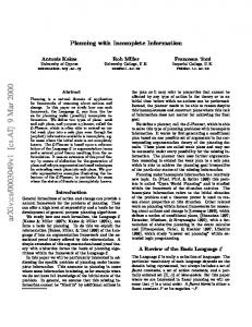
2.3 Actions An action describes the eects the plan operator has on the world when it is executed. The nature of the eects can depend both on the state in which the step is executed as well as random factors (not modeled in the state). Figure 1 shows a diagram of the paint action: an error results if an attempt to paint the widget is made when it has already been processed; otherwise with probability 0.95 the widget will become painted and all blemishes removed and with probability 0.05 the action will not change the state of the world at all. Notice that the leaves of the tree do not contain states; rather they indicate changes to a state (like strips adds and deletes). paint PR p(0.95) α

PA BL

PR p(0.05) γ

β

ER

Figure 1: The paint action usually paints the widget (PA) and removes blemishes (BL). We can describe an action formally as a set of consequences. Each consequence is a triple of the form hT i ; pi; E i i, where T i is a set of domain propositions known as the consequence's trigger, pi is a probability, and E i is a set of eects associated with the consequence. The representation for the paint action is paint

= f (fPRg, 1.0, fERg) (fPRg, 0.95, fPA, BLg) (fPRg, 0.05, fg) g

The changes resulting from a set of eects E is de ned by a function result(E ; s) in the manner of a strips add and delete list: negate all the propositions that appear negated in E then remove negations from all propositions that appear in E without negation (see [Kushmerick et al., 1993] for the full de nition). An action induces a change from a state s to a probability distribution over states, which we de ne in terms of the probabilities that its consequences will occur. First of all, for any consequence hT i; pi; E i i we de ne P[hT i ; pi; E i ij s] = P[T i j s] 2 pi (5) Notice that T i is a set of domain propositions, therefore P[T i j s] will be either 0 or 1 for any state s, and so this probability will either be 0 or pi for any consequence. Furthermore, we require the triggers of an action to have following two properties:



an action's triggers T are mutually exclusive and exhaustive, so for any state s one trigger will have probability 1 and the rest will have probability 0,



for any single trigger T i , the associated probabilities pj will sum to 1. 4

ship

reject

PR

PR

FL α

PR

FL β

PR

PR

FL γ

PR ER

α

ER

PR

FL β

PR ER

γ

ER

Figure 2: The ship and reject actions As a result we know that hT i ; pi; E i i2A P[hT i ; pi; E i ij s] = 1 for any action A and any state s. The tree-structured form of our actions (e.g. Figure 1) makes it easy to construct actions which have these properties. Now we can de ne the probability that executing an action A starting from state s results in a new state t: P

P[t j s; A] =

(

P[hT i ; pi; E i ij s] if hT i ; pi; E i i 2 A and t = result(E i ; s) 0 otherwise

(6)

The form of an action's consequences noted above guarantees that t P[t j s; A] = 1 for any action A and any state s. In the example scenario the distribution after executing paint looks like this: P

2

P2fFL; BL; PR; PA; ERgj ~sI ; P2fFL; BL; PR; PA; ERgj ~sI ; P2fFL; BL; PR; PA; ERgj ~sI ; P fFL; BL; PR; PA; ERgj ~sI ;

3

= 0:285 paint = 0:015 3 paint = 0:665 3 paint = 0:035 paint

3

And given this probability distribution we can compute the marginal probabilities of various combinations of domain propositions. For example: P[fPAgj ~sI ; paint] = 0:95 P[fBLgj ~sI ; paint ] = 0:015 P[fPR; ERgj ~sI ; paint ] = 0:0 P[fFLgj ~sI ; paint ] = 0:3 Figure 2 shows two more actions pertaining to the example: ship and reject. The ship successfully processes the widget if it is not awed and not already processed. Shipping a awed widget or trying to ship a widget that has already been processed will cause an execution error. The reject step works similarly: the step processes the widget successfully if it is awed and it has not already been processed.

2.3.1 Action sequences

We will often reason about executing a sequence of actions|we will use hA1; A2 ; : : :; An i to mean executing A1, then A2 , and so on, and hi to mean a sequence of 0 actions. State probabilities after executing a sequence of actions are de ned as an extension of Equation 6: P[u j s; hi] =

(

1 if u = s 0 otherwise 5

(7)

X

P[u j s; hA1 ; A2; : : : ; An i] =

t

P[t j s; A1 ] 2 P[u j t; hA2; : : : ; An i]

(8)

2.4 Information-producing actions We have so far represented actions as a mapping from a state to a probability distribution over states, where the new distribution is de ned by the eects the action will have on the world if it is executed in the input state. By contrast consider an action inspect that reports on whether or not the widget is blemished (whether or not BL is true). We want to retain the de nition of actions as mappings from mutually exclusive triggers into sets of eects, but we also want to distinguish between the eects the action has on the world and the eects it has on the agent's state of information [Etzioni et al., 1992]. Executing inspect does not change the probability that BL is true, but it does provide the agent with information about whether BL is true or not. Executing inspect and receiving a report that BL is true does change BL's posterior probability, but the nature of that report will not be known until the step is actually executed. We model the information produced by an action by allowing it to report on which of its consequences actually occurred at execution time. We do so by placing an observation label on each of an action's consequences. The observation label corresponds to the sensor's report: when the action is executed the agent will be informed of the observation label of the consequence that was actually realized in the world. There is an important distinction between our representation and the approach employed by other sensing representations (e.g. [Peot and Smith, 1992]), which assert the results of a informationgathering act just as if the information-gathering act had made the result true. Confusing the changes an action makes to the world with the changes an action makes to the agent's information about the world can lead to anomalous behaviors, like attempting to make a proposition true by repeatedly sensing it. c-buridan avoids this and similar diculties, since inserting an informationproducing action into a plan does does not change the probability that the observed proposition is true when the the plan is executed. However the conditional probability that the observed proposition is true given that a particular report has been received does change, as we will explain below. inspect BL

BL p(0.10)

α

β OK

p(0.90) γ

OK

BAD

Figure 3: The inspect action models an imperfect sensor Consider the inspect action in Figure 3.2 There are two dierent observation labels, \BAD", and \OK". Also notice that two consequences are labeled with \OK", so the agent would be unable to ascertain which of these two consequences actually occurred.

This version of inspect is overly simple in that it allows the widget to be inspected after it has been processed. A more realistic version of the action would have a fourth consequence with trigger PR, which would make ER true. 2

6

The observation labels must be included in an action's de nition, so now an action's consequence consists of four parts: hT i ; pi ; E i ; oii, where T i is the trigger, pi is the probability the consequence will be realized if the trigger is true, E i is the eects the consequence will have if it is realized, and oi is the observation label reported if the consequence is realized. Information-producing actions are those with more than one observation label; the information they convey is de ned by their discernible equivalence classes, or decs, indicated by the ovals in Figure 3. Actions like paint have no informational eect|they have a single observation label attached to all their consequences, thus they have a single dec. Executing the action provides no information as to which consequence actually came about. Notice the dierence between the causal and informational eects of executing an action. The changes an action makes to the world are recorded in the change sets of its consequences, and the planner uses the contents of the actions' eect sets when adding steps and links to a plan. Although the actions in our example problem are either essentially causal in their eects (paint) or informational in their eects (inspect ), there is no reason that an action cannot both change the world and provide information about it as well|an action can have both propositions in its change sets and more than one observation label, and the planner can exploit both of these properties. The immediate information provided by the execution of inspect can be characterized as follows: if it generates the report \BAD" then consequence de nitely occurred and BL is de nitely true, but if it generates the report \OK" then either  or occurred, and BL may or may not be true. We can characterize the inspect action more precisely using these conditional probabilities that appear in the action's consequences: P[2\BAD" j BL]3 P \BAD" j BL

= 0:9 = 0:0

P[2\OK" j BL]3 P \OK" j BL

= 0:1 = 1:0

which is a standard probabilistic representation of an uncertain evidence source (see, e.g., [Pearl, 1988, Chapter 2]). The probabilities of domain propositions conditioned on sensor reports is handled using Bayes rule in the standard way. Suppose inspect is executed in the initial state (where PR is known to be false and P[BL] = 0:3), and the report \OK" is received: P[BL j \OK"] =

(0:1)(0:3) P[\OK" j BL]P[BL] 2 3 2 3 = = :041 (0:1)(0:3) + (1:0)(0:7) P[\OK" j BL]P[BL] + P \OK" j BL P BL

If instead the report \BAD"is received: P[BL j \BAD"] =

(0:9)(0:3) P[\BAD" j BL]P[BL] 2 3 2 3 = = 1:0 (0:9)(0:3) + (0:0)(0:7) P[\BAD" j BL]P[BL] + P \BAD" j BL P BL

The inspect action can also provide information about propositions other than BL. Since BL and FL are initially perfectly correlated in the example, we have P[FL j BL] = 1 and therefore can conclude P[FL j \BAD"] = 1 and P[FL j \OK"] = 0:041. Executing paint destroys this correlation, however, so executing inspect after paint would not provide any additional information about FL(but it still would about BL). The point is that the information content of an action cannot be fully characterized by examining the operator alone|it depends on what probabilistic relationships hold in the plan at the time the action is executed. Finally we should note that sensing actions like inspect are useless by themselves: the fact that the probability of FL changes depending on whether inspect reports \OK" or \BAD" is of no use to 7

the planner if it can't make the execution of subsequent plan steps sensitive to which of the two reports are received. Section 3.4.1 discusses how the execution of steps in a plan can depend on the observation labels generated by previous steps.

2.5 Plan steps & contexts

A plan step is a triple: haction; index; contexti. The step index allows multiple instances of the same action to appear in the plan, in particular allowing their observation labels to be distinguished. Suppose that there were two instances of inspect in a plan, one with index i, the other with index j . The two observation labels of the rst step would be \OK-i" and \BAD-i" while the second step's observation labels would be \OK-j" and \BAD-j." Our example plans will have only one instance of any action, so we will omit these indexes in the paper. A step's context dictates the circumstances under which the step should be executed. In particular, each context is a set (implicit conjunction) of observation labels from previous steps in the plan; only when the step's context matches the observations actually produced during execution can it can be executed. Suppose, for example, we have the following sequence of steps:

hinspect; 1; T i, hship; 2; f\OK"gi hreject; 3; f\BAD"gi and suppose the agent executes the inspect step, receiving the report \BAD". It then considers executing the next step in the sequence. It skips ship, since that step's context does not match the report produced by execution of inspect . The agent next decides to execute the third step, reject, since the step's context does match the report produced by inspect . In summary, we require that an agent keep track of the execution context|the reports (observation labels) produced by the steps executed in the plan so far. Plan steps are executed only when the execution context matches the step's context.

2.6 Assessing goal probability

Here we de ne the probability that the a sequence of steps satis es some goal expression G . The de nition is an extension of Equation 8 that takes into account each step's context and its relation to previously executed steps in the sequence. In particular, the eect of executing a step given an execution context is either (i) the eect of executing the corresponding action (if the contexts match) otherwise, (ii) no change (if the step's context doesn't match the execution context). To make this precise, we start with the analogue of Equation 7, stating that if there are no steps in the sequence then the probability depends only on the initial probability. Here C is an execution context (a conjunction of observation labels), and the probability computed is that the world will be in state u after a particular sequence of steps is executed, given that the execution context is C and that the world is currently in state s. P[u j C; s; hi] =

(

8

1 if u = s 0 otherwise

(9)

Next, if the rst step in a sequence is not executable it does not change any probabilities, nor does it change the execution context. Recall that both the step's context and the execution context are boolean combinations of observation labels, so we can de ne \executability" in terms of logical entailment: S is executable in context C just in case C ` context(S). P[u j C; s; hS1 ; S2 ; : : : ; Sn i] = P[u j C; s; hS2; : : : ; Sn i] if C 6` context(S1)

(10)

Finally, if a step is executable in the current context it changes both the probability distribution over states and the execution context, both according to its set of consequences action(S) = fhT i; pi; E i; oiig: P[u j C; s; hS1 ; S2 ; : : : ; Sn i] = X P[hT i ; pi; E i ; oiij s]P[u j (C ^ oi ); result(E i ; s); hS2; : : : ; Sn i] hT i; pi; E i; oii2action(S1) if C ` context(S1 )

(11)

2.7 Planning problems and solutions A planning problem consists of:

 

A probability distribution over initial states ~sI . A goal expression G |a set (conjunction) of domain propositions describing the desired nal state of the system.

 A set of actions like paint, inspect, ship, and inspect, de ning the agent's capabilities.  A probability threshold  specifying a lower bound on the success probability for an acceptable plan.

The planning algorithm produces a sequence of steps hS1 ; : : : ; Sn i, where each step is an instance of an action along with the circumstances under which the action should be executed. Such a sequence is a solution to the problem if the probability of the goal expression after executing the steps is at least equal to the threshold. In other words, hS1 ; : : :; Sn i solves the planning problem just in case P[Gj ~sI ; hS1; : : : ; Sn i]   . Section 2.6 de nes this probability. 3

Plans and planning

Our planner takes a problem (initial probability distribution, goal expression, threshold, set of actions) as input and produces a solution sequence|a sequence of steps whose probability of achieving the goal exceeds the threshold. Here we describe its data structures and the algorithm it uses to produce a solution.

9

goal initial p(0.7) α

FL BL PR ER PA

PR ER PA

p(0.3) β

FL BL PR ER PA

α “success”

Figure 4: The initial plan

3.1 Initial and goal steps The planner initially converts the problem's initial and goal states into two steps, initial and goal. The initial step codes the initial probability distribution, and the goal step has a single consequence with the goal state as its trigger. Figure 4 shows initial and goal actions for the example.

3.2 Plans

Following buridan [Kushmerick et al., 1993], the planner manipulates a data structure called a plan, consisting of a set of steps, ordering constraints over the steps, and a set of causal links. The initial and goal actions each appear exactly once in every plan, with the initial step ordered before all others and the goal step ordered after all others. A plan with only these two steps and this single ordering is called the initial, or null plan, and is the algorithm's starting point.

3.2.1 Causal links Causal links record decisions about the role the plan's steps play in achieving the goal. A link connects a consequence of a \producing" step with a proposition p in a trigger of a \consuming" step. A causal link makes explicit the dependency between the two steps, recording the fact that increasing the probability of the producing step's designated consequence will tend to increase the probability that p will be true when the consuming step is executed, which will tend to make the plan more likely to succeed.3 For example, the planner might create a link from the  consequence of a paint step to the PA trigger proposition of the goal step, indicating that paint is supposed to make PA true for use by PA goal. We will use the notation paint  ! goal to refer to this link. p More generally the notation Si! Sj refers to a link whose producer is consequence  of Si , which produces proposition p for Sj .4 Since the goal expression appears in the plan as a set of triggers in the single consequence of the goal step, planning to achieve the goal proceeds by adding steps that produce the goal propositions and linking from the appropriate consequences of these steps to the goal step, then creating links to the triggers of these new consequences as well. 3 We say that adding links will \tend" to increase the probability of success because the circumstances under which two links will produce the desired result can be correlated, hence there is no guarantee that adding a link will increase the probability of the supported proposition. For example, suppose a link records a desire to make p true, but its producing step will do so only if some other proposition q is true. Now suppose we create a second link to make p true, but it too does so only if q is true. Adding the second link does not increase the probability that p will be true: either both links will generate p or neither will. Adding multiple links to the same consuming proposition can never decrease the probability that it will be true, but the possibility of correlation with other links means that it might not4increase the probabilityth either. We will refer to the j step in a plan either with the notation Sj , or by using its name, e.g. paint. Referring to a step by name is not generally a good idea since there could be several steps with the same name in the plan. However, since our example has only one step for each action, there is no ambiguity.

10

3.2.2 Subgoals A plan's links determines a set of subgoals for the planner, each a pair of the form < p; Sj >, where p is some proposition and Sj is some step in the plan. The presence of such a pair indicates that raising the probability that p is true at the time Sj is executed will tend to increase the probability that the plan will succeed. A pair < p; Sj > is a member of a plan's subgoals just in case either

 j is the index of the goal step and p is a member of the problem's goal expression G (meaning that p is one of the explicit goals of the planning problem), or



is a proposition in one of the triggers of an consequence  of Si , and the plan contains a link q S for some S and some proposition q. of the form Si! j j p

In other words, the subgoals represent the set of propositions that participate in chains of causal links ending at the goal. We will introduce additional subgoals in Sections 3.3.2 and 3.4.1.

3.2.3 Threats to links The process of adding steps and links to the plan can generate con icts. Suppose that a plan p S . The link actually represents two commitments on the planner's contains a link of the form Si! j part: (1) to make Si realize its consequence , resulting in p becoming true, and (2) to keep p true from Si 's execution until Sj 's execution. Therefore any step that 1. possible occurs after Si , and 2. possibly occurs before Sj , and 3. has an eect that makes p false pS. is called a threat to the link S ! i

j

3.2.4 Summary The plan data structure consists of a set of steps, a set of ordering constraints, and a set of

causal links. Every plan contains the initial and goal steps that describe the planning problem. From a plan's links one can compute a set of subgoals and a set of threats. The subgoals indicate propositions in the plan for which adding additional links might make the plan more likely to succeed. The threats indicate con icts in the plan that might prevent success. Planning therefore involves creating links to subgoal propositions and resolving threats to those links. We call these two options the possible re nements to the plan.

3.3 The planning algorithm Here is a brief description of the planning algorithm: 1. Begin with the null plan, containing only steps and no causal links. 2. Iterate: 11

initial

and

, the ordering (initial < goal),

goal

(a) Assess the current plan: compute the probability that the current plan achieves the goal. Report success if that probability is at least as great as the threshold. (b) Otherwise nondeterministically choose a re nement to the current plan. Report failure if there are no possible re nements. Otherwise apply the re nement to the current plan and repeat. Any implementation of the algorithm will of course have to manage the nondeterministic choice using backtracking or some other search technique.

3.3.1 Assessment A plan de nes a partial order over its steps, which in turn de nes a set of legal execution sequences. Calculating the probability that such a set of steps could achieve a goal is a complex task. Here, we present a very simple algorithm for performing this calculation, based closely on the de nition of step execution. The algorithm simply iterates over all step sequences consistent with the plan's ordering constraints. For each totally ordered sequence, the algorithm calculates the probability distribution over the states that could possibly result. When it has nished iterating over the steps in a particular total order, it sums the probabilities of all the states in the distribution in which the goal is true. If the probability is greater than  , the algorithm returns the successful sequence, otherwise it continues to the next total order. If no sequence has a success probability greater than  the assessor reports failure. The probability distribution is represented as a set of triples (sj ; pj ; cj ) where sj is a state as de ned in Section 2.2, pj is a probability, and cj is a context (as de ned in the previous section). Context cj is the conjunction of all the observation labels that were observed in the execution that produced state sj . For each totally ordered sequence hS1; : : :; Sn i consistent with the plan: 1. Initialize fringe := f(si , pi , T)g where P[~sI = si ] = pi is the initial probability distribution provided by the user and T is a context that is always true.

2. Loop for S = S1 ; S2 ; : : : ; Sn : (a) Loop for (sj ; pj ; cj ) 2 fringe: i. When cj ` context(S) do: A. Remove (sj ; pj ; cj ) from fringe B. Loop for (T i ; pi; E i ; oi) 2 action(S): Add to fringe the triple (result(E i ; sj ); pj 2 pi 2 P[T i j sj ]; cj ^ oi ) 3. If 

 Pf(sj ; pj ; cj )2fringeg pj 2 P[Gj sj ] then return hS ; : : :; Sni. 1

The algorithm computes the probability distribution over states generated by each action in the sequence, nally summing the probabilities of all nal states in which the goal is true. This simple version of plan assessment is often quite inecient; we include it here only to keep the presentation simple. [Kushmerick et al., 1993] discusses four dierent plan-assessment algorithms and compares their performance. One of the most interesting assessment algorithms presented in that paper uses the plan's set of causal links to estimate the success probability without enumerating any total ordered sequences. 12

3.3.2 Re nement A plan re nement adds structure to a plan, trying to increase the probability that the plan will achieve its goal expression. Recall that the probability of goal achievement can be increased in one of two ways:

 if < p; Si > is a subgoal, then adding a new link from some (possibly new) plan step to this proposition might increase the probability that p is true at Si , and therefore might increase the success probability,



if a causal link is currently part of the plan but some other step in the plan threatens the link then eliminating the threat might increase the probability of the link's consumer proposition, and therefore might increase the success probability.

Adding links and steps to the plan is the same as for deterministic causal-link planners: for some p S can be inserted for any existing pair < p; Sj > selected to be the link's consumer, a link Si! j step Si that can be ordered before Sj and whose consequence  asserts p, or between any new step with a consequence  that asserts p, where the new step is constrained to occur before Sj . However, notice that the existence of a link to a trigger proposition does not ensure that the proposition will be true|that will depend on whether or not the producing consequence is actually realized. As a result the planner needs to be able to introduce multiple links to a proposition to try to increase the probability that it will be true. Threat resolution in c-buridan is also similar to threat resolution in deterministic causal-link planners. Promotion and demotion (i.e., the addition of ordering constraints on the threatening steps) works in precisely the same way as in the deterministic case. Two additional threat-resolution mechanisms, confrontation and branching, have no analogue in classical planning, however. Confrontation was introduced in the buridan probabilistic planner and is adopted without change from that system [Kushmerick et al., 1993]. The idea behind confrontation is that a plan can be suciently likely to work even if some action in the plan makes a goal or subgoal false, as long as the falsifying consequence of that action is suciently unlikely to occur. Since the consequences of any action are mutually exclusive, the planner can make a particular consequence of an action less likely to occur by making a dierent consequence of that same action more likely to occur. If consequence  of some step St threatens a link by making p false, then the threat can be confronted by choosing some consequence of St that does not make p false and adopting its trigger as a subgoal. The last way of resolving threats is called resolution by branching, and has no analogue in classical planning or in buridan. We explain the details in Section 3.4.1, but provide a brief overview here. Intuitively, branching ensures that the agent will never execute the threatening step when the link's consuming step is depending on an eect of the link's producing step. Resolution by branching works by making the context in which St occurs incompatible with the context in which the link proposition is required by the link's consumer. In summary, the algorithm's re nement phase consists of nondeterministically choosing to work on a subgoal or to resolve a threat: 1. Choose either a subgoal to support or a threatened link to protect. 2. If the choice is a subgoal of the form < p; Sj >, choose some step Si whose consequence  asserts p. Si must either be a new step (instance of an action), or an existing step in the plan p S to the plan, and order (S < S ). that can be ordered before Sj . Add the link Si! j i j 13

!p Sj threatened by some consequence of a step St, then choose to

3. If the choice is a link either

   

Si

(demote) add the ordering (St < Si ) to the plan, (promote) add the ordering (Sj < St) to the plan, (confront) choose some consequence  of St that does not contain p and adopt the trigger of St as a subgoal, or (branch) restrict the context of St so it is incompatible with either the context of Si or Sj .

3.4 Example Recall that the example problem consists of



An initial probability distribution over states, which is converted to an initial plan step (Figure 4).



A goal expression fPR, PA, ERg (the widget should be processed and painted, and the plan should not have an error). The goal expression is converted to a nal plan step (again Figure 4).

 

A set of actions:

,

,

paint reject ship

, and inspect (Figures 1, 2, and 3.)

A success threshold of  = 0:8.

The initial set of subgoals consists of the goal propositions: f< PR; goal >; < PA; goal >; < ER; goal >g. Suppose the planner makes the following choices. First it supports < ER; goal > with a link from consequence  of initial. Next it supports < PA; goal > by adding a step paint, linking its  consequence to the goal, thus adopting < PR; paint > as a subgoal, since PR is a trigger for the  consequence. This pair can in turn be supported by a link from the initial step. Now < PA; goal > has probability 0.95 of being true but the plan has success probability 0 because PR is false. Next the planner supports < PR; goal > by adding a ship step, linking its  consequence to the goal, and as a result two new pairs, < FL; ship > and < PR; ship >, become subgoals. Both of these pairs can be linked to the initial step's  consequence. The resulting partial plan has three threats:



! paint is threatened by ship, in particular its  and consequences. (In The link initial PR other words, ship might make PR true, but paint requires it to be false.)



! goal is threatened both by paint (consequence ) and by ship(consequences The link initial ER and ).

The rst threat can be resolved by demoting the ship step, ordering it after paint. The second two threats cannot be resolved by adding ordering constraints: no step can be ordered before the initial step or after the goal step, so these two threats must be confronted or branched. Suppose the planner decides to use confrontation. The planner chooses non-threatening consequences for each step: ship and paint , notes in the links that the threat was confronted ( initial ship ER ;paint! goal), and adopts 

14



initial p(0.7) α

p(0.3) β

FL BL PR ER PA

FL BL PR ER PA

paint PR p(0.95) α

PA BL

PR p(0.05) β

γ

ER

ship PR

PR

FL α

PR

FL β

PR ER

γ

ER

goal PR ER PA α “success”

Figure 5: A plan with success probability 0:665 as subgoals the triggers of the non-threatening consequences: < PR; ship >, and < PR; paint > (as it happens, both were subgoals already). Figure 5 shows the resulting plan. Temporal ordering among the steps goes from top to bottom: initial < paint < ship < goal, links appear as arrows from consequence boxes to trigger propositions, and confronted threats appear as arrows from the non-threatening consequence (e.g. ship ) to the ! goal). threatened link ( initial ship ER  ;paint This plan, which is the one that the non-contingent planner buridan would produce, will work just in case the widget is initially not awed and the paint step works, which translates into a success probability of (0:7)(0:95) = 0:665. The success probability can be increased somewhat by adding additional paint steps to raise the probability that PA will be true, but without introducing information-producing actions and contingent execution no planner can do better than 0.7. At this point a reasonable re nement to the plan in Figure 5 would be to support the pair < PR; goal > by adding a reject step and linking it to the goal. The problem with this strategy is that it introduces a pair of irreconcilable threats: reject makes PR true, which threatens the link from initial to ship , and likewise ship makes PR true, threatening a link from initial to reject. Adding orderings can resolve only one of these two threats, and confronting the threat means that the planner will be trying to make reject's  consequence come true (so it will produce PR for the goal) 15

and simultaneously trying to make reject's consequence come true (so it won't produce PR before ship is executed). It cannot do both successfully, since any two consequences of a single action are mutually exclusive, so decreasing the probability of one threat increases the probability of the other. This plan appears in Figure 6, with threatened links appearing in grey. The solution is to execute one or the other (but not both) depending on the state of FL. initial state p(0.7) α

p(0.3) β

FL BL PR ER PA

FL BL PR ER PA

paint PR

PR

p(0.95) α

ship PR

PR

γ

β

PA BL

ER

PR

FL α

p(0.05)

FL β

PR ER

γ

ER reject PR

PR

FL α

PR

FL β

PR ER

γ

ER

goal state PR ER PA α “success”

Figure 6:

ship

and reject threaten each other

Here the need for information gathering and conditionals becomes apparent: the planner needs to be able to insert steps that provide information about the state of FL and needs to be able to make the steps executed in the plan depend on that information. We next introduce a method for resolving threats based on making the context of the participating steps incompatible, i.e. by making context(Si ) ^ context(Sj ) ^ context(St ) unsatis able.

3.4.1 Threat resolution by branching We call this new threat-resolution strategy \branching" because we will introduce contingency branches into the plan that prevent the threat from materializing.5 Branches are a new element in

[Peot and Smith, 1992] refers to this approach as \conditioning." We adopt an alternative term because of a possible confusion with the use of the term in probabilistic reasoning, e.g. \conditioning on new evidence." 5

16

a plan's structure, analogous to causal links. A branch connects an information-producing step to a subsequent step, indicating the observation labels of the rst that enable execution of the second. We will add two branches to our example plan: inspect=f\OK"g)ship and inspect =f\BAD"g)reject. The rst means that ship should be executed only if the execution of inspect generates an observation label of \OK", the second means that reject should be executed only if the execution of inspect generates an observation label of \BAD". These restrictions are realized by adding the appropriate observation label to the steps' contexts. p S by branching is as follows: The general procedure for resolving a threat St to a link Si! j 1. Choose to make context(St ) incompatible with either context(Si ) or context(Sj ). Let Ss be the step chosen. 2. Choose some information-producing step Sp that can be ordered both before Ss and before St . Sp must also be executable in some context compatible with both S s and St , that is, context(Sp )^context(Ss )^context(St ) must be satis able. Sp need not be in the plan already| it can be added to the plan in order to resolve the threat. 3. Choose a set c = fc1; : : : cn g and a disjoint set c0 = fc01 ; : : :c0 m g of Sp 's observation labels. 4. Add ordering constraints to the plan: (Sp < Ss ), (Sp < St ) 5. Add branches to the plan: Sp=c)St and Sp =c0)Ss 6. Make step contexts more restrictive:

 

context(St ) := context(St ) ^ (c1 _ c2 : : : _ cn ) context(Ss ) := context(Ss ) ^ (c01 _ c02 : : : _ c0m )

7. Add to the plan's subgoals all pairs of the form < p; Sp >, where of Sp's triggers.

p

is any proposition in any

3.5 Example Return now to the example which progressed as far as Figure 6|the planner had added both ship and reject steps in order to raise PR's probability over 0.7. Doing so led to a threat (both ship and reject require PR to be false initially and make it true) that could not be resolved by ordering or by confrontation. This threat can be solved by branching, however. Suppose that the planner rst ! ship. notices that the reject step is threatening the link of the form initial PR 1. It chooses to make the contexts of the link's consumer incompatible.

ship

and the threatening step

reject

2. It chooses an information-producing action inspect and adds it to the plan. 3. It chooses subsets of inspect 's observation labels: c = f\BAD"g, c0 = f\OK"g. 4. It adds ordering constraints to the plan, (inspect < reject), (inspect < ship), ensuring that the information-producing step will be executed before the actions whose contexts depend on its observation label. 17

5. It adds branches inspect =f\OK"g)ship and inspect=f\BAD"g)reject to the plan. 6. It restricts the steps' contexts as follows:

 

context(reject) := T ^ f\BAD"g = \BAD" context(ship) := T ^ f\OK"g = \OK" initial p(0.7) α

p(0.3) β

FL BL PR ER PA

FL BL PR ER PA

inspect BL

BL p(0.10)

α

paint PR p(0.95) α

PR

PR

BAD

γ

β

ER

OK PR

FL α

OK

p(0.05)

PA BL

ship

γ

β OK

PR

p(0.90)

FL β

PR ER

reject γ

PR

ER FL α

PR

BAD PR

FL β

PR ER

γ

ER

goal PR ER PA α “success”

Figure 7: A successful plan Now ship and reject are restricted to mutually exclusive execution contexts, and the plan is shown in Figure 7. The resulting plan admits two execution sequences:

 

inspect paint

, then paint, then ship or reject,

, then inspect , then ship or reject.

The rst sequence has success probability .9215: it will fail only if the paint step fails or if the widget was blemished and the inspect step incorrectly reports \OK". The second sequence has success probability 0.665, however: when paint is executed it makes BL false with probability .95, 18

(and with probability 0.05 it fails to make PA true, which means the plan will fail anyway). In any execution path in which paint succeeds, it will also make BL false, which means that inspect will certainly report \OK", and the widget will be shipped regardless of whether or not it was initially

awed. The assessment algorithm in Sections 3.3.1 and 2.6 will nd and return the high-probability sequence, and the planner will terminate successfully. It is interesting to note, however, that the planner could further re ne this plan, adding an ordering constraint so only the high-probability sequence is valid. How can the planner recognize and eliminate the bad sequence? Recall that all the trigger propositions of the inspect step are subgoals at this point|in particular, the planner can choose to support < BL; inspect > with a causal link from the initial step's consequence. Then paint will threaten the link, since its  consequence makes BL false. One way this threat can be resolved is by ordering paint to come after the link's consumer, ordering it after inspect . The resulting plan has only one consistent ordering: inspect then paint then ship or reject, which has success probability 0.9215.

3.6 Contexts and plan structures At this point we should mention a novel feature of our method of inducing conditional plan execution using restricted step contexts introduced by branching: the fact that our algorithm can generate plans whose executions \branch" then \rejoin." Suppose, for example, that we added an additional goal condition to the plan, that the planner notify a supervisor when it nished processing a widget. Assume that notify's single precondition is that the widget be processed (PR). c-buridan can handle this easily, inserting the notify step along with a link from its single outcome to the goal step, then creating links from both ship and reject's  consequences to its trigger condition PR (see Figure 8). Note that since notify's execution context is T because it participates in no threats, so the execution sequence represented by this plan is inspect , paint, either ship or reject, notify. Other conditional planners, e.g. cnlp and Warplan-C [Warren, 1976] generate a new plan branch each time a conditional is inserted in the plan, and do not allow the branches to contain common steps. BAD reject

T init

T

T

inspect

notify

paint

goal

OK ship

Figure 8: A plan with merged branches

4

Propagation of Step Contexts

The c-buridan planning algorithm described in the previous section restricts a step's context only when doing so is necessary to resolve a threat. This policy produces correct plans, but admits ineciency. Suppose, for example, that the ship action had an additional precondition HB (have box), and the planner had an additional operator get-box that had no preconditions and made HB 19

true. At some point the planner would insert a get-box step in the plan and link it to ship, resulting in the situation pictured in Figure 9(a). Notice that get-box's context will be unrestricted since it causes no threats nor is its link threatened by any other steps. Get-box will therefore be executed in all contexts, including those contexts in which reject will be executed instead of ship. We might want to restrict the context of this step so it is executed only when it is \useful," which in this case means in exactly those contexts in which ship is executed. T

OK

get-box

ship

T inspect

OK

OK

get-box

ship

T

OK

inspect

(a)

OK

(b)

Figure 9: Restricting have-box's context so that it is only executed when needed. Since a step's reasons for being in a plan are recorded in the plan's link structure, we look there to determine when a step is useful. A step S is useful in a plan only when:

 

At least one of the steps that produces propositions it consumes is executed, and At least one of the steps that consumes propositions it produces is executed.

If the rst condition is not true, no previous step in the plan will produce the state that S requires to be eective, and since S can't do anything useful it might as well not be executed. If the second condition is not true then no subsequent step will be able to exploit whatever eects S was put in the plan to accomplish, therefore it might as well not be executed. If we allow a step's context to be an arbitrary boolean expression (rather than a simple conjunction as assumed previously), we can constrain a step's context as follows:



A step's context should at least be restricted to the disjunction of the contexts for all the steps that act as producers of causal links consumed by that step.



A step's context should at least be restricted to the disjunction of the contexts for all the steps that act as consumers of causal links produced by that step.

The rst constraint is enforced by a forward propagation of contexts through the plan whenever a new link or branch is added. The second constraint is enforced by a backward propagation sweep through the plan before it is returned as a solution. The second constraint allows us to restrict the context of get-box to be only \OK" (Figure 9(b)), since its only link in the plan is to ship, and ship 's context is restricted to circumstances in which inspect reports \OK".

4.1 Forward propagation Forward propagation enforces the rst constraint by computing a step's context as follows: let

B = the set of branches pointing to S, 20

then,

C = the set of consequences of S, T (c) = the set of trigger conditions for consequence c; P (t) = the set of steps producing links to trigger condition t;

context(S) = (

^

b2B

branchlabel(b))

^(

_

^

_

c2C t2T (c) p2P(t)

context(p))

where branchlabel(b) is the set of observation labels associated with branch b. The rst clause represents the context information dictated by S's immediate branches (i.e. those assigned when it was involved in threat resolution by branching). The second clause formalizes the de nition above: it is the disjunction of the contexts of all steps that produce propositions consumed by S's trigger propositions. The context of a step S is recomputed whenever a new link or branch is made to it, and changes to its context are propagated recursively to the consumers of all links for which S acts as producer. Notice that adding a new causal link to S can actually \widen" S's execution context (i.e. the step can be executable in more contexts as it consumes more links), and when a step's context widens it can threaten links that it did not threaten before. So whenever a step's context is changed, the algorithm must also check to see whether the step poses new threats to any links currently in the plan.

4.1.1 Empirical implications of context propagation We noted initially that context propagation was not necessary to produce successful plans| foregoing the propagation phase means at worst that some steps might be executed unnecessarily in some contexts. We then introduced the propagation algorithm that is run every time a link or branch is added to a plan, one that requires traversing the plan's link structure and scanning it for new threats as well. The question therefore arises whether this additional computational step is worth the eort|perhaps the forward propagation should be performed only once, after a successful plan is built, to make sure its steps are executed only when necessary. While it is an open empirical question as to whether frequent context propagation is a good idea, we should point out an additional bene t of context propagation: its potential to make the plan-generation process itself more ecient. Recall that propagation serves to restrict a step's context, and that a step can threaten a link only if its context is compatible with the link's context. Therefore restricting a step's context can serve to eliminate threats that would otherwise have to be resolved by the planner.

4.2 Reverse propagation Forward propagation ensures that an action will only be executed when its causal links can in fact provide support for those consequences necessary for plan success. Reverse propagation, on the other hand, ensures that an action will only be executed when one of its consequences is actually needed|the context of a step S is conjoined with disjunction of the contexts of S's consumers. There is an added restriction however: if S's context expression mentions an observation label \L", then S must be ordered after the step that generates \L". For example, in Figure 9, get-box must be ordered after inspect , since its new context is derived from that step. If the plan's ordering 21

constraints do not permit this ordering, then all occurrences of the observation label \L" must be removed from S's context. The algorithm for reverse propagation is therefore as follows: 1. Let < S1; : : : Sn > be a sequence of steps representing a consistent ordering of the steps in plan P 2. Loop for S= Sn , Sn01 , : : : , S1 : (a) Let C be the set of steps that consume either links or branches from S. W (b) context(S) := context(S) ^ clean( c2C context(c)) (c) Order S after all the steps that generate observation labels that appear in context(S) where clean(expr) removes from expr all the observation labels produced by steps that cannot be ordered before S.

4.2.1 Reverse propagation and completeness One big dierence between forward and reverse context propagation is that the latter actually adds ordering constraints to the plan. Forward propagation restricts a step's context, but does not add additional structure (links or orderings) to the plan. Ordering constraints are added during plan re nement when links are created and when threats are resolved|both are necessary to preserve the probabilistic dependency between a link's producer and its consumer. Reverse context propagation, on the other hand, can order a step Sp after a sensing step Ss not because Sp's execution should directly depend on the consequent of Ss , but because Sp is a link producer for some third step Sc whose execution does depend on the result of Ss . Ordering S p after Ss prevents the planner from later deciding that Sp should be ordered before, so after reverse propagation Sp could never produce a link consumed by Ss or any prior step even though semantically there is no reason why it could not do so. A planner that performs reverse propagation on every partial plan (i.e. after every plan re nement) is therefore incomplete. Once again the question of whether and when to do reverse context propagation is an open empirical question|one can either perform reverse propagation on every partial plan and accept the incomplete algorithm as a concession to eciency, or alternatively a planner could run the reverse propagation algorithm only once as a post-processing step, once a successful plan has already been found. Reverse propagation does not change the plan's probability of success, so it cannot make a successful plan unsuccessful. 5

Summary and Related work

c-buridan is an implemented algorithm for plan generation that combines information-producing actions with a framework that allows the conditional execution of actions. Novel features of the representation include:



The representation allows planning with actions whose eects and information content depend on both the prevailing world state and random chance.

22



The action representation can encode a variety of senor models, including anything from asymmetrically noisy sensors to sensors that provide complete and awless information about the world.



The representation for information-producing actions is a natural extension of symbolic planning operators, yet admits a traditional Bayesian semantics for representing the information content of an action and for updating belief on the basis of observation.



Causal and informational eects of an action can be combined arbitrarily|there is no distinction made between sensing and eecting actions.



The framework allows reasoning about informational dependencies: the fact that an action can provide indirect information about the state of the system, and the fact that other actions can create or destroy dependencies among state variables.



Our approach to restricting step contexts does not require tree-structured plans|plans can diverge initially in their execution contexts, then rejoin to execute steps that are needed in several contexts.



While we have not proven that the c-buridan algorithm is complete, it can solve problems that stumped buridan and ones that cnlp could not solve.

5.1 Related work Related work in conditional planning includes work in decision analysis as well as previous probabilistic planners and AI work on (deterministic) conditional planning.

5.1.1 Decision analysis The concept of planning to gather information (and assessing the value of that information) is a common topic in the Decision Analysis literature, particularly the work on sequential decision making [Winkler, 1972]. Our approach uses the same Bayesian framework, but the emphasis is dierent in that we take our task to be one of building a good plan automatically from schematic action descriptions and an input problem. Work in decision analysis is generally more concerned with structuring the problem, eliciting domain and preference models from experts, and evaluating alternatives provided by experts rather than on algorithmic approaches to generating those alternatives. Graphical structures like in uence diagrams can be used to solve sequential decision-making problems, including those that allow information-gathering steps [Matheson, 1990]. We do not consider in uence diagrams a solution to the planning problem in and of themselves, however| they do not address the problem of generating plans from action schemas and problem descriptions.

5.2 Probabilistic planning

Our work extends the buridan planner [Kushmerick et al., 1993]: we added to buridan the idea of information-producing steps and step contexts, as well as the threat-resolution technique of branching (which is due to cnlp, see below), and the algorithms for context propagation. See [Kushmerick et al., 1993] for a discussion of related probabilistic planning algorithms. 23

5.3 Conditional planning

Our approach to contingent planning borrows much from the cnlp algorithm of [Peot and Smith, 1992]. In particular we adapted their method of threat resolution by conditioning: that informationproducing actions generate execution contexts, and that one way to resolve a threat is to force the threatening step and the threatened link to appear in mutually exclusive contexts. cnlp and c-buridan use dierent underlying representations. cnlp adopts a standard strips (logical) semantics, whereas our c-buridan n manipulates a probabilistic representation. Our inspect action would look like this in cnlp: Name: Observe-widget Pre: Unk(blemished) (not (processed)) +a1: (blemished) +a2: (not (blemished))

(It seems as though the rst precondition, that the state of blemished be unknown, is not necessary|it indicates that it will never be useful to insert a step into a plan if (1) its only eect is to provide information about a proposition and (2) the state of that proposition has already been determined previously in the plan.) Observation labels in c-buridan play the same role as in cnlp|the annotations +a1 and +a2 above represent reports the sensor might produce at execution time, which are used in building execution contexts for subsequent steps. cnlp's action model cannot represent a situation in which an operator performs dierently depending on the prevailing world state or on unmodeled (chance) factors. cnlp therefore cannot model sensing operators like our inspect operator, whose behavior is state dependent and noisy. The fact that actions have multiple possible consequences complicates the planning process somewhat: since a link to a proposition does not guarantee the proposition's truth, we have to admit the possibility of multiple (disjunctive) causal support for propositions, and a step's context can contain disjunctions as well (whereas in cnlp a step's context is a conjunction of observation labels). Our algorithm for introducing contingencies diers from cnlp as well: cnlp's approach is based on the idea that every time a new execution context is introduced into the plan (by conditioning or branching) a new instance of the goal step is also added with that context. The planner thus tries to build a plan that satis es all instances of the goal step, i.e. a plan that will work under all circumstances. The resulting plans are tree-structured: once two branches in the plan are created to condition on possible sensor reports, subsequent steps in separate branches cannot share steps. We noted in Section 3.6 that our algorithm can represent plans in which certain steps (like ship and reject ) should be executed in restricted execution contexts, but that subsequent steps (like notify) should be executed unconditionally.

5.4 Future work Our preliminary work on c-buridan has produced a good framework for posing the problem of conditional and informational planning, but the system is limited both by its representation and by its computational eciency. Future work in the following areas is therefore indicated:

24

Computational properties Our initial experiments with buridan showed us that the compu-

tational complexity of building probabilistic plans is signi cantly worse than building plans using a logical representation language. And the problem becomes worse still when the planner can insert information-gathering actions and conditionals. To put it bluntly, while c-buridan is fully implemented, signi cant search control knowledge is necessary to enable solution of even simple examples like the one presented in this paper. Consider the question of when it might be advantageous to insert an information-producing action into a plan. It can be dicult to ascertain exactly what propositions a particular sensing action provides information about. Recall from the example above that the inspect operator provides direct information only about whether the widget is blemished, but the planner really cares only about whether the widget is awed. Information about BL turns out to convey information about FL in this particular case, but the relationship depends on the particular planning problem and indeed even the particular plan being constructed|the information content of an sensing operator cannot be determined by examining the operator alone. The basic computational problem is that any information-producing action can potentially provide information about any proposition. A practical planner will need fast heuristic methods for deciding what information it needs to gather in order to build a successful plan, and what information-producing operators are likely to provide it with that information.

More expressive languages c-buridan's utility is limited by its propositional representation language. Related work is concerned with building and reasoning about plans using more expressive representation languages: [Hanks, 1993] explores the problem of assessing a plan's quality, but using a probabilistic framework that allows reasoning about sets and quantities. [Golden et al., 1993] is an eort to incorporate a richer sensing model, based on uwl [Etzioni et al., 1992], into the ucpop partial-order planner. Its inference rules allow eective reasoning about locally complete information, enabling the planner to satisfy universally quanti ed goals under incomplete information, and to eliminate redundant sensing operations. Value of information c-buridan generates a plan with a particular probability of success. It is more common to analyze both plans and information-producing actions within plans in terms of their utilities or values: a value or utility model associates a value with a plan, then an informationproducing action can be evaluated in terms of the value it contributes to a plan. [Matheson, 1990] demonstrates how to evaluate plans in this way, but does not provide an algorithm for generating plans. [Haddawy and Hanks, 1993] point out that planning to maximize the probability of goal success corresponds to planning to maximize expected value only for a particular extremely restricted class of utility models. c-buridan must therefore be extended to generate plans according to a criterion of expected-utility maximization, at which point information-gathering actions can be evaluated in terms of the utility they add to the plan. We intend to apply the framework for utility models developed in [Haddawy and Hanks, 1993] to this planner, but doing so rst requires extensions to the representation language as noted above. Formal properties We need to complete proofs that the (nondeterministic) c-buridan algo-

rithm is sound and complete. We can use the formal framework developed to prove these properties for non-contingent buridan, but need to extend the plan semantics to account for information25

gathering actions and branches. Previous work [Etzioni et al., 1992] contains a compatible semantics for contingent plans, but uses a non-probabilistic language. We also need to explore the relationship between our algorithm and algorithms from the decision sciences like value iteration [Howard, 1960] and other dynamic programming approaches [Raia, 1968]. References

[Allen et al., 1990] J. Allen, J. Hendler, and A. Tate, editors. Readings in Planning. Morgan Kaufmann, San Mateo, CA, August 1990. [Etzioni et al., 1992] Oren Etzioni, Steve Hanks, Daniel Weld, Denise Draper, Neal Lesh, and Mike Williamson. An Approach to Planning with Incomplete Information. In Proceedings of KR-92, October 1992. Available via anonymous FTP from ~ftp/pub/ai/ at cs.washington.edu. [Golden et al., 1993] K. Golden, O. Etzioni, and D. Weld. xii: Planning for Universal Quanti cation and Incomplete Information. Technical report, University of Washington, Department of Computer Science and Engineering, To Appear 1993. [Haddawy and Hanks, 1993] Peter Haddawy and Steve Hanks. Utility Models for Goal-Directed Decision-Theoretic Planners. Technical Report 93{06{04, Univ. of Washington, Dept. of Computer Science and Engineering, September 1993. Available via anonymous FTP from ~ftp/pub/ai/ at cs.washington.edu. [Hanks, 1993] Steve Hanks. Modeling a Dynamic and Uncertain World II: Action Representation and Plan Evaluation. Technical report, Univ. of Washington, Dept. of Computer Science and Engineering, September 1993. [Howard, 1960] Ronald A. Howard. Dynamic Programming and Markov Processes. MIT Press, 1960. [Kushmerick et al., 1993] N. Kushmerick, S. Hanks, and D. Weld. An Algorithm for Probabilistic Planning. Technical Report 93-06-03, Univ. of Washington, Dept. of Computer Science and Engineering, June 1993. Submitted to AIJ. Available via anonymous FTP from ~ftp/pub/ai/ at cs.washington.edu. [Matheson, 1990] James E. Matheson. Using In uence Diagrams to Value Information and Control. In R. M. Oliver and J. Q. Smith, editors, In uence Diagrams, Belief Nets and Decision Analysis, pages 25{48. John Wiley and Sons, New York, 1990. [Pearl, 1988] J. Pearl. Probablistic Reasoning in Intelligent Systems. Morgan Kaufmann, San Mateo, CA, 1988. [Peot and Smith, 1992] Mark A. Peot and David E. Smith. Conditional Nonlinear Planning. In Proceedings of the First International Conference on AI Planning Systems, pages 189{197, June 1992. [Raia, 1968] Howard Raia. Decision Analysis: Introductory Lectures on Choices Under Uncertainty. Addison-Wesley, 1968. 26

[Warren, 1976] D. Warren. Generating Conditional Plans and Programs. In Proceedings of AISB Summer Conference, pages 344{354, University of Edinburgh, 1976. [Winkler, 1972] Robert L. Winkler. Introduction to Bayesian Inference and Decision. Holt, Rinehart, and Winston, 1972.

27