in a partial motion planner, and the probability of collision is updated in ... the information and the planning under uncertainty problem is solved using Markov ... car-like constraints. ... environment is initially unknown and the robot explores it and builds .... inference. In a first case we will consider that the moving obstacles are.
Probabilistic Rapidly-exploring Random Trees for autonomous navigation among moving obstacles. Chiara Fulgenzi, Anne Spalanzani, and Christian Laugier LIG, INRIA Rhˆone-Alpes, France Abstract— The paper presents a navigation algorithm for dynamic, uncertain environment. The static environment is unknown, while moving pedestrians are detected and tracked on-line. The planning algorithm is based on an extension of the Rapidly-exploring Random Tree algorithm, where the likelihood of the obstacles trajectory and the probability of collision is explicitly taken into account. The algorithm is used in a partial motion planner, and the probability of collision is updated in real-time according to the most recent estimation. Results show the performance for a car-like robot among a pedestrian tracking dataset and simulated navigation among multiple dynamic obstacles.
I. I NTRODUCTION Autonomous navigation in populated environments represents still an important challenge for robotics research. The key of the problem is to guarantee safety for all the agents moving in the space (people, vehicles and the robot itself). In contrast with static or controlled environments, where path planning techniques are suitable [1] [2], high dynamic environments present many difficult issues: the detection and tracking of the moving obstacles, the prediction of the future state of the world and the on-line motion planning and navigation. The decision about motion must be related with the on-line perception of the world and take into account the sources of uncertainty involved: 1) The limits of the perception system: occluded zones, limited range, accuracy and sensibility, sensor faults; 2) The future behaviour of the moving agents: model error, unexpected changes of motion direction and velocity; 3) New agents entering the workspace; 4) Errors of the execution system. Many real world applications rely on reactive strategies: the robot decides only about its immediate action with respect to the updated local estimation of the environment [3]–[5]. These strategies present however some major drawback: first of all the robot can be stuck in local minima; secondly, most of the developed approaches do not take into account the dynamic nature of the environment and the uncertainty of perception, so that the robot can be driven in dangerous or blocking situations. To face these problems, reactive techniques are combined with global planning methods: a complete plan from present state to goal state is computed on the basis of the a priori information; during execution, the reactive algorithm adapts the trajectory in order to avoid moving and unexpected obstacles [6]–[8]. If the perception invalidates the planned path
replanning is performed. In all the cited methods however, uncertainty is usually not taken explicitly into account. From the more theoretical point of view instead, many works handle a non-deterministic or probabilistic representation of the information and the planning under uncertainty problem is solved using Markov Decision Processes (MDP), Partially Observable MDPs or game theory [9]–[11]. For an overview see [2]. These approaches are however very expensive from the computational perspective, and are limited to low dimensional problems or to off-line planning. In [12] and [13] a navigation strategy based on typical pattern based and probabilistic prediction is used in a planning algorithm based on a complete optimization method, A∗ . However, the problem of A∗ and of all complete methods is that the computational time depends on the environment structure and obstacles: these methods are more adapted to a low dynamic environments, where the information does not change frequently, the obstacles velocity is limited and the robot can stop often and plan its future movements. Also, they require a discretization of both the state and the control space, which reduces drastically the space for finding a feasible solution, expecially for robots with non-holonome or car-like constraints. Some recent work proposes to integrate uncertainty in randomised techniques, such as Probabilistic Road Maps [14] and Rapidly-exploring Random Trees (RRT) [15] [16]. In a highly dynamic environment an anytime algorithm is needed, which is able to give a feasible solution at ”anytime” it is asked to. In this paper we address the problem of taking explicitly into account the uncertainty in sensing and in prediction. We want our navigation algorithm to integrate new information coming from the perception system and to be able to react to the changes of the environment. In previous work [17] we developed a probabilistic extension of the RRT algorithm to handle a probabilistic representation of the static environment and of the moving obstacles prediction. The search algorithm has been integrated in a navigation algorithm which updates the probabilistic information and chooses the best partial path on the searched tree. The navigation algorithm is based on the architecture of Partial Motion Planning (PMP, [18]), where execution and local planning work in parallel to assure safe behaviour. The static environment is initially unknown and the robot explores it and builds an occupancy grid. While in [17] motion patterns were represented by Gaussian Processes, in this paper we consider two cases: in the first case the obstacles are simply tracked and their motion model is estimated on the basis of
previous observations; in the second case, the obstacles are supposed to follow pre-learned motion patterns which are represented by Markov chains and prediction is based on Hidden Markov Models. The reminder of this paper is structured as follows: section III describes the representation of the static and dynamic world and how the probability of collision of a configuration is computed. Section IV recalls the RRT basic algorithm and details the new proposed approach. Section V recalls the PMP method and describes the planning and navigation algorithm developed. Results are presented in Section VI: an experiment with a laser scan dataset with moving pedestrians is presented and results in a simulated environment are shown. Section VII ends the paper with remarks and ideas for future work. II. T HE ROBOT
AND THE
S TATE S PACE
We consider a car-like robot moving in R2 . The configuration space C = {x, y, θ, v, ω} described respectively by the position, orientation, linear and angular velocities of the robot in the workspace. The robot moves according to its motion model q(t + 1) = F (q(t), u(t)) where input u is given by pairs (a, α) with a the linear and α the angular acceleration. The robot is subjected to kinematic and dynamic constraints: the linear velocity v is limited in the interval [0, vmax ] and the angular velocity ω is limited in [−ωmax , ωmax ]. a and alpha are also bounded: a ∈ [amin , amax ] and α ∈ [αmin , αmax ]. Time is represented by the set T = (0, +∞), which is the infinite set of discrete instants with measure unit the timestep τ . We define state space X of the robot, the space that represents the configuration of the robot at a certain instant in time X = C × T . In the workspace there are static and moving obstacles. The task of the robot is to move from the initial configuration q0 to a goal configuration qgoal in finite time without entering in collision with any obstacle. A solution trajectory is a sequence of states from q0 to qgoal that is feasible according to the motion model of the robot and that is collision free: ie each configuration and each transition of the sequence are collision free. We assume that the position of the robot is known at each instant and that the robot moves following according to its motion model without error. In the deterministic case, the configuration space C can be divided in Cf ree , the set of free configurations of the robot and Cobs , the set of configurations where the robot is in collision with an obstacle. In our case instead we want to give a probabilistic representation of environment perception and prediction uncertainty and we need to define a probability of collision for each robot configuration. In the following paragraphs we explain how this probability is computed for a considered state of the robot Xr . III. P ROBABILITY
OF COLLISION
A. The Static environment The 2D static environment is represented by an occupancy grid [19]: the space is divided in square cells. The environment is initially unknown, and the probability of
(a)
(b)
Fig. 1.
(a) The cycab in the parking at INRIA Rhˆone-Alpes and (b) an occupancy grid with the robot (green rectangle) and 2 moving obstacles (coloured circles) along with their estimated trajectories.
occupation Pocc of each cell is fixed at 0.5. During navigation the space is observed by mean of a distance sensor (laser range finder). Assuming static environment, the probability of occupation of each cell is recursively updated according to the observations and estimated using a Bayesian filter. The probability of collision of a point in the space is given by the probability of occupation of the correspondent cell. For the set S = (i, j)N of N cells covered by the robot in state Xr , the probability of collision with static obstacles is given by the maximum probability over the set: P (coll(Xr , G)) = max(Pocc (i, j)) S
(1)
Since the grid represents the static world, there is not need of prediction and the probability of collision does not depend on the time at which the robot is in a certain configuration. B. Moving obstacles Lets assume that the moving obstacles Oi can be approximated by circles of fixed radius. The state of an obstacle is X = (x, y, θ, v), its position in the 2D space, its orientation and linear velocity. Given an object observation Z, the belief state X and the prediction are estimated using Bayesian inference. In a first case we will consider that the moving obstacles are detected and tracked by the robot using a Multi Hypothesis target Tracking (MHT) algorithm based on a set of Kalman Filters as in [20]: the motion of the obstacles can be represented with M linear motion models hypotheses Am , each affected by zero-mean white Gaussian noise N (0, Qm ). At a considered instant t, the estimation of the state of an object is represented by a weighted sum of Gaussians (Gaussian mixture): P (Oi (t)) ←
M X
ˆ m (t), Σm (t)) αm · N (X
(2)
m=1
ˆ can be analytically computed from the The prediction X last estimation applying recursively the motion model. The obtained distribution is always a mixture of M Gaussians. Considering time horizon t + k: ˆ m (t + k) = Am · Xm (t + k − 1) = Ak · X(t) X (3) ˆ + k) = (AT )k · Σm (t) · Ak + Σ(t m m
k X (Ajm · Qm ) j=0
(4)
Considering a state of the robot Xr (t) and a moving obstacle Oi , the probability of collision is given by the integral of the probability distribution over the area S covered by the robot and enlarged by the radius of the obstacles: ZZ P (coll(Xr , Oi )) = P (coll(Xr , Oi )) = S M X
=
αm
m=1
ZZ
ˆ t , Σt ) N (X m m
(5)
S
The integral in previous equation is approximated sampling the distribution uniformly with the probability and considering the ratio between the number of samples inside and outside area S. In a second case we will consider obstacles moving according to Hidden Markov Models as in [21]. The belief of the state at time t is given by a discretized distribution over the states of the Markov model. The prediction at time horizon t+k is recursively estimated propagating the estimated state: P (X(t + k)|Z(t)) = X
based on some assumptions about the observed space and the size, shape and behaviour of the obstacles. The robot must be able to recognize on-line the doors with its perception only. In the parking environment where we tested our algorithm, we assumed that obstacles may enter only traversing hidden areas: i.e. they cannot pass through static obstacles. Given a partial map and the point of view of the robot, these regions are easily extracted: the distance between the the points on the scan is studied and intervals bigger than the minimal size of an obstacles are kept as possible doors. For each interval, the partial map is observed to see if the area around is occupied, free or occluded. If the area is occupied, the considered interval is discarded: the area is occupied by a static obstacle that is hidden only from the current point of view. If the area is free or occluded (Pocc ≤ 0.5), a door is recognized. The probability of a new obstacle entering in the workspace can be modeled as an homogeneous Poisson process. The probability that at least one obstacle enters the scene, is given by the following equation: P [N (t + τ ) − N (t) ≥ 1] = 1 − e−λτ
P (X(t + k)|X(t + k − 1))P (X(t + k − 1)|Z(t))
X(t+k−1)
where the first term in the sum is the probability to pass from state X(t + k − 1) to state X(t + k) specified by the edges in the Markov model and the second is given by the observation model. The integral in Eq. 5 is here substituted by the sum over the states in the HMM touched by the area S. Considering multiple moving obstacles, the total probability of collision is given by the probability of colliding with one OR another obstacle. Under the assumption that collisions with each obstacle are conditionally independent, the following equation is obtained: Y (1 − P (coll(Xr , Oi )) (6) P (coll(Xr , O)) = 1 −
(8)
The rate parameter λ, is the expected number of arrivals per unit time. This parameter could be derived from a learning phase or fixed a priori. When performing prediction, an obstacle is initialized just behind the door, in the nearest possible point with respect to the robot actual position. The probability of occupation correspondent to the obstacle grows with the length of the time period of prediction according to Eq. 8. Using a worst-case hypothesis, obstacles are supposed to move toward the robot. A noise in both direction and a velocity is added to the model to take into account the other possibilities of motion.
i
In the same way the probability of collision considering both the static environment and the moving obstacles is obtained: P =
(coll(Xr , O, G)) = (7) 1 − (1 − P (coll(Xr , G)) · (1 − P (coll(Xr , O)))
C. New obstacles entering the scene In dynamic environments, obstacles can enter or exit the workspace during the navigation task. Also if partial planning is used, it should be taken into account that new obstacles can enter the the workspace and interfere with the next motions of the robot. If it is possible to predict from where and when some obstacle may enter the scene, a more robust planning can be performed. The robot must: – Distinguish from where a new obstacle may come. – Apply a probability to the fact that an obstacle may enter and a motion model. For the first problem the robot searches for specific areas from where an obstacle may enter (doors). This technique is
Fig. 2.
A partial grid map, the extracted doors and the supposed new entering
obstacles.
IV. P ROBABILISTIC RRT S A. Basic Algorithm for RRTs The Rapidly-exploring Random Tree (RRT) is a well known randomized algorithm to explore large state space in a relatively short time. The pseudocode of the algorithm is given in Algorithm 1. The algorithm chooses a point p in the state space and tries to extend the current search tree toward that point. p is chosen randomly, but in single-query planning, some bias toward the goal is generally applied in
(a)
(b)
(c)
Fig. 3. (a) RRT basic algorithm applied to a point holonome robot in a known static environment; (b) Perception given by a distance sensor at the initial position: white, black and grey represent respectively free, occupied and occluded zones; (c) Probabilistic RRT built in limited time: the search tree and the likelihood of the nodes in blue (lighter colour is for lower likelihood) and the chosen partial path in red.
B. Introducing probabilistic uncertainty As stated in previous sections, the robot knowledge about the environment is incomplete in both space and time (sensor range, occlusions, new moving obstacles) and uncertain (sensor accuracy, motion model of the moving obstacles). On the basis of the RRT algorithm we developed an exploring algorithm which takes into account probabilistic uncertainty. For each configuration q of the space, a probability of collision Pc (q) is computed considering the static and moving obstacles and the perception limits as in Eq. 7. The probability of reaching a particular configuration qN is then given by the probability to cross the tree from the root q0 to the considered node, i.e. the probability of not having collision in each of the traversed nodes: Ps (π(qN )) Ps (q0 ...qN )
Algorithm 1: 1 2 3 4 5 6 7 8 9 10 11 12 13
Basic RRT.
Data: T while qgoal ∈ / T do p = ChoosePoint (qgoal ); q = T. NearestNeigbohr (p); qnew = extend (q, p); if qnew ∈ Cf ree then T. addSon (q, qnew ); end q = qgoal ; path = add (q); while q 6= T.root do q = T. parentNode (q); path = add (q); end
order to speed up the exploration. p is chosen in the limited Cf ree (line 2). The nearest neighbour q of p within the nodes of the search tree is chosen for extension. A new node is obtained applying an admissible control from the chosen node q toward p (line 3). If q is collision-free, it is added to the tree. The algorithm can be stopped once the goal is found (line1) or it can continue to run to find a better path. The algorithm lies on a deterministic representation of the environment, so that both in the static and dynamic case we have a priori information on if a node is collision free or not and add it or not to the search tree. Once the goal state is reached, the path from the initial state to the goal is retrieved. Fig. 3(a) shows a point holonome robot in a known environment with static obstacles. The initial position of the robot is in the left corner at the bottom while the goal is in the upper right corner. An example of the search tree (blue lines) and the found path (red line) is shown; different running of the algorithm would give different results. In this case, the robot is supposed to move along straight lines, so that the Euclidean distance can be used to determine the nearest neighbour in the current tree. The algorithm can be generalized for car-like robots setting a different NearestNeighbor(. ) function. and limiting the set of possible actions to the admissible controls of the robot from the node configuration.
= Ps (q0 ...qN ) = (1 − Pc (qN )) · Ps (q0 ...qN −1 ) N Y = (1 − Pc (qn ))
(9)
n=0
where we have considered that collision in subsequent nodes is statistically independent. We call this probability the probability of success Ps of the path. The probability falls exponentially with the length of the path. This is a sign that longer path are more dangerous, as the uncertainty accumulates over subsequent steps. All nodes than can be added to the tree, or a minimum threshold Psmin1 can be chosen in order to avoid keeping in the tree very unlikely paths. Once a point p is chosen in the configuration space, the node to grow next q is chosen in dependence both on a measure of the expected length of the path dist(q0 , q, p) and on the probability of success of the path. More precisely, Ps (qN ) is normalized by the length N of the path and multiplied by the inverse of the distance to the chosen point. p 1 N Ps (q) (10) w ˜q = dist(q0, q, p) w ˜q (11) wq = P ˜q qw The normalization is taken out so that the probability of success does not depend on the length of the path, which is taken instead into account by the distance term. The function dist(q0 , q, p) is a sum of the length of the path from the root q0 to the considered node and of the shortest path from q to p, which is a lower limit for the length of the eventual path to p. The obtained weights w ˜q are normalized over the set of nodes in the tree (Eq. 11), and the result is a distribution over the nodes. The node to grow next is chosen taking the maximum or drawing a random node proportionally to the probability. In our implementation we choose the second case which appeared to be more robust to local minima. Even if a path to the goal is found, the algorithm can continue to search for a better/safer path, until a path is asked for execution. However, it is not guaranteed that a safe enough path is found even in infinite time, because of the environment uncertainty. The chosen path is then the best path that is safe enough, i.e. for which Ps (qN ) ≥ Psmin2 .
(a)
(b)
(c)
Fig. 4.
Partial Probabilistic RRT applied to static environment for a point nonholonome robot. The tree updated and grown at three instants during navigation (in blue) and the chosen partial path (in red).
In general, this threshold is different from Psmin1 : when the tree is updated and grown after new observations (see §sec:OnLineNavigation) the probability of each path is infact modified. Fig. 3(b) shows the perception given by a distance sensor in a static environment: areas behind the obstacles are unknown to the robot ( Pc ≃ 0.5). Fig. 3(c) shows the tree grown by the described algorithm for an holonome point robot. The colour of the edges of the tree depends on the likelihood of the associated path: the lighter the colour the lower the likelihood. In red, the best path chosen. V. O N - LINE
NAVIGATION
A. Related work: the Partial Motion Planning In a dynamic environment the robot has a limited time to perform planning which depends on the time-validity of the models used and on the moving objects in the environment. The conditions used for planning could be invalidated at execution time: for example an obstacle could have changed its velocity or some new obstacle could have entered the scene. The idea of Partial Motion Planning [18] is to take explicitly into account the real-time constraint and to limit the time available for planning to a fixed interval. After each planning cycle, the planned trajectory is generally just a partial trajectory. The exploring tree is updated with the new model of the world and the final state of the previous trajectory becomes the root of the new exploring tree. The planning algorithm works in parallel with execution. Each node of the tree is guaranteed to be not an Inevitable Collision State (ICS, [22]) by checking if it exists a collision free braking trajectory from the node. This is a conservative approximation that does not allow the robot to pass an intersection before an approaching moving obstacle. Our approach presents an adaptable time horizon for planning. The time for the planning iterations depends on the length of the previous computed trajectory and on the on-line observations. Safety of a path is guaranteed studying braking trajectories only for the last state of the path. B. Developed Algorithm When the robot moves, it observes the environment and updates its estimation with the incoming observations. The
cost of crossing the tree changes and the tree needs to be updated. The update consists in three steps: 1) Prune the tree: the new root is the position of the robot and nodes that are in the past are deleted; the probability of reaching the nodes is updated, taking into account that the robot has already crossed part of the tree. 2) Update the weight of the nodes: when a change in the probability of collision is detected, the weight of the correspondent nodes (and of their subtree) must be updated. 3) Retrieve the best path. If the considered environment is dynamic we need the robot to do these operations in real-time. In better words we need to know how much time is available for updating and how to allocate it. In the first step, the present state of the robot is considered. The tree is pruned so that only the subtree attached to the state of the robot is maintained. When the probability to pass from a configuration q0 to qi changes, the weight of the subtree attached to qi is updated using the following equations: P (qN |qi ) P (qN |q0 )
1 (12) ˆ 1 − P (qi |q0 ) = P (qi |q0 ) + (1 − P (qi |q0 ))P (qN |qi ) (13)
= (P (qN |q0 ) − Pˆ (qi |q0 ))
The first equation gives the probability of traversing the tree from qi to qN , assuming that the probability of reaching qi changed from Pˆ (qi |q0 )) to 1: q0 is the old root, qi is the new root and qN is a node in the family of qi . This first update is used when the tree is pruned and is due to the fact that the robot has already moved from q0 to qi , so that the new P (qi |q0 ) is 1. The second equation gives the probability to traverse the tree from q0 to qN when the probability to pass from q0 to qi changes from 1 to P (qi |q0 ). Eq. 12 and 13 are used one after the other when the observations revealed some difference with the prediction. In this case q0 and qi are respectively the start and ending configuration in which a change in the probability of collision has been detected. In Fig. 4, the on-line updating of the tree is shown at 3 instants during navigation. At the beginning, the most likely paths are explored in the two possible directions and the most promising one is chosen. Fig. 4(b) shows the tree after some steps: the tree has been updated: the branch in the right direction has been cut has is not reachable anymore and the tree has been grown. Fig. 4(c) shows the tree and the new partial path found when a bigger portion of the space is visible VI. E XPERIMENTAL R ESULTS The planning algorithm has been tested with real data acquired on the car-like vehicle (Cycab) shown in Fig. 1(a). To test the algorithm we define a goal 20 meters ahead the robot at each observation cycle and let the algorithm run in parallel with the online mapping and tracking (Fig. 6(b)). The planning algorithm runs at 2Hz. An example of the grown tree and the chosen path is shown in Fig. 5. The occupancy
Fig. 5.
(a)
(b)
(c)
(d)
(e)
(f)
The prediction of the moving obstacles and the explored tree in (x, y, t)
space.
grid correspondent to the figure is the one in Fig. 1(b). The two cones represent the prediction of the two moving pedestrians considering ellipses of axes correspondent to one standard deviation interval. A threshold has been applied to show different colours for safer (green) and dangerous (red) paths. The best path is shown in blue. Each sequence is then tested with the real data, letting a virtual robot move through the map. Fig. 6(a) shows the observed occupancy grid (a) and the tree of states explored in the available time (b): lighter blue is for higher probability of collision. The red line is the chosen path. Fig. 6(c-f) shows subsequent positions of the virtual robot; on the background the predicted occupancy grid at the correspondent planning stage, while the red circles represent the real position of the obstacles at the considered time. Results prove that the algorithm is able to compute safe trajectories in real time taking into account the static environment, the moving obstacles perceived and their velocity and the uncertainty which arises from a real dataset. The navigation strategy has been tested in the Cycab simulator (7(a)). A rectangular environment has been simulated. A certain number of doors is simulated for the two long sides of the rectangle. Obstacles are supposed to enter from a door and to exit by another door in the opposite side. The space has been discretized in a uniform cell grid of step 0.5m An 4-connected HMM graph has been built on the grid for each goal: the probability to pass from a state to another depends on the decrease of the distance to the goal between the origin state and the destination one. A certain amount of noise is applied so that states that present nearly the same decrease in distance are given the same probability. The probability is then normalized over the set of edges coming out from the origin node. A set of trajectories has been randomly simulated on the basis of the graph: for each trajectory the enter door and the exit door are chosen (Fig. 7(b)). Given a state of the obstacle, the next state is drawn proportionally with the edges probability. The position of the obstacle inside the cell is chosen by a smoothing filter. The simulated robot has the same dimensions and kinematic and dynamic constraints of the Cycab. Perception is assumed
Fig. 6.
Planning results with a laser dataset. (a) The static environment is mapped and the moving obstacles are tracked. (b) The algorithm explores the state space and chooses a path. (c-f) the path is compared with the prediction and the real observations acquired.
perfect: the obstacles are represented by circles of 0.30m radius whose position is always known; no occlusion or finite range is considered. The robot has to cross the environment and successively reach goals which are positioned randomly in the environment, with some bounds near the walls. The robot knows where the doors are and the Markov graph correspondent to the simulated trajectories. Prediction is performed on the basis of Hidden Markov Models, as in [?] or [21] and the probability of collision is computed sampling the obtained distribution on the cells. Fig. 7(c-f) show the robot (green rectangle) traversing the environment to reach the goal: the red line is the partial path computed at the time-step in the shot, while red circles represent the moving obstacles with their previous trajectory attached. The robot reached 1000 goals with various numbers of pedestrians simulated in the space. No collision with the robot in motion was detected during the experiment, while the number of collisions as 0 velocity grows with the number of objects in the space. To understand these results, we must notice that the simulated obstacles do not have any knowledge of the
R EFERENCES
(a)
(b)
(c)
(d)
(e)
(f)
Fig. 7. Navigation results in simulated environment. (a) The Cycab simulator with the robot and simulated pedestrians. (b) The simulated trajectory dataset. (c-f) Navigation among moving pedestrians based on HMM probabilistic prediction.
robot and that its kinematic possibilities are strongly limited if compared to those of the obstacles: as the robot cannot go backward, it tends to avoid obstacles and get stacked with the walls of the environment, while the obstacles continue to move around it. VII. C ONCLUSION
AND FUTURE WORK
The paper presents a navigation algorithm which integrates perception uncertainty and incompleteness in the planning strategy using a probabilistic framework. The tests prove that the robot is able to navigate in real-time reacting properly to unexpected changes of the environment and reaching the given goal positions. The use of an adaptable time horizon for planning makes the algorithm both reactive to unexpected changes of the environment and forward looking when previously planned trajectories are not invalidated by observation. Immediate work will deal with testing the navigation algorithm to have a measure of its performance in more complex and realistic scenarios. Future work will deal with the integration of the localization and execution uncertainty in the planning algorithm and with testing the navigation with the real robot.
[1] J. C. Latombe, Robot Motion Planning. Dordrecht, The Netherlands: Kluwer, 1991, vol. SECS 0124. [2] S. M. LaValle, Planning Algorithms. Cambridge University Press (also available at http://msl.cs.uiuc.edu/planning/), 2006. [3] J. Borenstein and Y. Koren, “The vector field histogram - fastobstacle avoidance for mobile robot,” IEEE Transaction on Robotics and Automation, vol. 7, no. 3, June 1991. [4] R. Simmons, “The curvature-velocity method for local obstacle avoidance,” in IEEE International Conference on Robotics and Automation, ICRA, 1996. [5] D. Fox, W. Burgard, and S. Thrun, “The dynamic window approach to collision avoidance,” IEEE Robotics & Automation Magazine, vol. 4, no. 1, Mar. 1997. [6] S. Quinlan and O. Khatib, “Elastic bands: connecting path planning and control,” in IEEE International Conference on Robotics and Automation, ICRA, 1993. [7] C. Stachniss and W. Burgard, “An integrated approach to goaldirected obstacle avoidance under dynamic constraints for dynamic environments,” in IEEE International Conference on Intelligent Robots and Systems, IROS, 2002. [8] F. Large, “Navigation autonome d’un robot mobile en environnement dynamique et incertain,” Ph.D. dissertation, Universit´e de Savoie, 2003. [9] R. Simmons and S. Koenig, “Probabilistic robot navigation in partially observable environments,” in Proceedings of the International Joint Conference on Artificial Intelligence (IJCAI ’95), July 1995, pp. 1080 – 1087. [10] S. LaValle and R. Sharma, “On motion planning in changing, partiallypredictable environments,” Int’l J. Robotics Research, vol. 16, pp. 775– 805, 1997. [11] A. Foka and P. Trahanias, “Real-time hierarchical pomdps for autonomous robot navigation,” Robot. Auton. Syst., vol. 55, no. 7, pp. 561–571, 2007. [12] M. Bennewitz and W. Burgard, “Adapting navigation strategies using motion patterns of people,” in In Proceedings of the IEEE International Conference on Robotics and Automation (ICRA. IEEE, 2003, pp. 2000–2005. [13] M. Bennewitz, W. Burgard, G. Cielniak, and S. Thrun, “Learning motion patterns of people for compliant robot motion,” The International Journal of Robotics Research (IJRR), vol. 24, no. 1, 2005. [14] P. Missiuro and N. Roy, “Adapting probabilistic roadmaps to handle uncertain maps,” in Proc. of IEEE International Conference on Robotics and Automation, 2006, pp. 1261–1267. [15] R. Benenson, S. Petti, M. Parent, and T. Fraichard, “Integrating perception and planning for autonomous navigation of urban vehicles,” in IEEE IROS, 2006. [16] N. Melchior and R. Simmons, “Particle rrt for path planning with uncertainty,” in IEEE ICRA, April 2007. [17] C. Fulgenzi, C. Tay, A. Spalanzani, and C. Laugier, “Probabilistic navigation in dynamic environment using rapidly-exploring random trees and gaussian processes,” Intelligent Robots and Systems, 2008. IROS 2008. IEEE/RSJ International Conference on, pp. 1056–1062, Sept. 2008. [18] S. Petti and T. Fraichard, “Safe motion planning in dynamic environments,” in IEEE IROS, 2005. [19] A. Elfes, “Using occupancy grids for mobile robot perception and navigation,” Computer, vol. 22, pp. 46–57, June 1989. [20] J. Burlet, “Adaptive interactive multiple models applied on pedestrian tracking in car parks,” 2008, phD thesis. [21] D. Vasquez, “Incremental learning for motion prediction of pedestrians and vehicles,” Ph.D. dissertation, INP de Grenoble, February 2007. [Online]. Available: http://emotion.inrialpes.fr/bibemotion/2007/Vas07 [22] T. Fraichard and H. Asama, “Inevitable collision states. a step towards safer robots?” in IEEE IROS, 2003.