Probabilistic Relational Scene Representation and ... - CiteSeerX

Probabilistic Relational Scene Representation and Decision Making Under Incomplete Information for Robotic Manipulation Tasks Rasoul Mojtahedzadeh, Abdelbaki Bouguerra, Erik Schaffernicht, and Achim J. Lilienthal ¨ Center of Applied Autonomous Sensor Systems (AASS), Orebro University, Sweden Abstract— In this paper, we propose an approach for robotic manipulation systems to autonomously reason about their environments under incomplete information. The target application is to automate the task of unloading the content of shipping containers. Our goal is to capture possible support relations between objects in partially known static configurations. We employ support vector machines (SVM) to estimate the probability of a support relation between pairs of detected objects using features extracted from their geometrical properties and 3D sampled points of the scene. The set of probabilistic support relations is then used for reasoning about optimally selecting an object to be unloaded first. The proposed approach has been extensively tested and verified on data sets generated in simulation and from real world configurations.

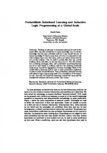
I. I NTRODUCTION There are many real-world environments where it is highly desirable to introduce robotic manipulation systems that have high degrees of autonomy. One example is the task of unloading goods stacked in shipping containers, where goods can come in random configurations. Fig. 1 shows two such difficult configurations of carton boxes inside cargo containers. To manipulate goods without damaging them, an autonomous robotic manipulation system needs to have two important abilities. First, it needs to create truthful models of the environment based on the available sensor data and task constraints. Second, it needs to be able to predict and reason about the effects of its actions based on the created models.

(a)

(b)

Fig. 1: Two example snapshots of chaotic configurations of carton boxes inside cargo containers. In this paper, we present a method to automatically build high-level symbolic representations that capture support relations between a set of detected objects under incomplete information about the scene configuration. The representation is then used for making decisions about which object to be

manipulated first so that a certain criterion is optimized (e.g., to minimize the risk of objects falling down). The work presented here is part of a larger research effort aiming at making the process of unloading shipping containers autonomous by relying on advanced cognitive abilities. The context of this work is the European Union project “Cognitive Robot for Automation of Logistic Applications” abbreviated to RobLog1 project. We build on previous work [1], in which we developed an approach to analyze configurations of solid objects in contact with each other in order to identify possible support relations between them. One assumption in that work is that the attributes of all the objects are given. Here, we relax this assumption, to address cases where only a subset of the objects in the scene are known. Such cases arise often in real-world environments where not all objects are detected. One case is when objects are not seen by the sensors due to occlusion. Another important case is when detection-andrecognition algorithms fail to recognize some of the objects even if they are in the field of view of the sensors. We consider only rigid objects with cuboid geometric shapes. For carton boxes, which are one of the most popular packagings for shipment of goods in containers [2], cuboids can be considered as a precise geometric description. Our approach can be coupled with any object detection algorithm capable of producing a set of attributes (i.e. type, size and pose) of a subset of the objects to be manipulated. We assume that information about geometrical attributes of the detected objects in addition to the raw 3D sensor data (e.g., a point cloud) of the scene are available. The main contributions of this paper can be summarized as follows: • A probabilistic model of the world that represents all possible support relations between the detected objects. • Utilizing a machine-learning method to estimate the probability of support relation between a pair of detected objects under incomplete information. • A decision making strategy for selecting an object, among the detected ones, with expected minimum cost. The paper is organized as follows. Related work is discussed in Section II. Section III outlines the different steps used to create probabilistic world models. Section IV covers the process of decision making given the probabilistic world model. Experimental results are reported in Section V, while section VI concludes the paper. 1 http://www.roblog.eu

II. R ELATED W ORK The problem of selecting an object to be manipulated by an automated industrial robot falls mostly in the category of “bin-picking” research. For an automated bin-picking system, it is desired to develop sophisticated algorithms to autonomously localize and manipulate objects by means of 3D range and visual perception. Bin-picking research follows two major tracks: the problem of object recognition and the problem of grasping. However, the problem of elaborately selecting the safest object to be manipulated in a randomly configured stack of objects and under incomplete information has received less attention. Papazov et al. [3] present an object recognition and pose estimation algorithm for grasping tasks of objects on tabletop scenes with simple physical interactions between objects. Their policy is to choose an object based on the distance of the center of mass to the table surface, i.e., the object with higher center of mass receives higher priority to be manipulated first. Chitta et al. [4] present an approach to mobile pick-and-place problems in which separated objects are standing on tabletop scenarios. Gupta and Sukhatme [5] present a pipeline which uses two simple motion primitives to sort and separate Lego bricks piled on a tabletop using the PR2 robot. Klingbeil et al. [6] present a method to autonomously grasp unknown objects with bar-code labels sitting on a tabletop scenario with simple configurations between objects. In all of the above works, scenarios with simple physical interaction between objects are considered. In our target scenario, configurations of objects inside shipping containers are unknown beforehand. Moreover, we have to deal with lack of information due to the fact that only a subset of the objects, in the configurations, are known. In our previous work [1], we created relational models of the configurations of objects by considering their geometrical and statics properties. However, that work relies on the assumption of the availability of complete information about all objects to be manipulated. III. P ROBABILISTIC S CENE R EPRESENTATION Given a static scene of a shipping container having a finite number of carton boxes arbitrarily stacked on each other, we assume that only a subset, D, of the carton boxes have been correctly detected and classified by a specialized module. We also assume that raw 3D sampled points of the scene are available. Our goal is to automatically generate a scene representation that captures possible support relations between the objects in D using their attributes (size and pose) and the scene point cloud. This representation can then be used by a reasoning module to select the object that satisfies a certain decision criterion (see Section IV). Support Relation. For two objects X and Y in a static configuration of objects, we say that X supports Y if removing X from the configuration causes Y to lose its motionless state (e.g., Y will fall down.). We denote this relation as SUPP(X,Y). A support relation can hold if the two objects are in direct or indirect contact with each other. Please note that it is possible to have configurations in which both

A

A

S

5

S9 S3

B

6

S

S2

S

A

S

S1

S4

D

S10

8

D

B

D

2

S1

7

B

1

S1 C

C

C

(a)

(b)

(c)

Fig. 2: Graph illustration of the vector W describing a world with four objects, where each edge k is labeled with a binary random variable Sk . Solid and dashed edges denote Sk = 1 and Sk = 0 respectively. (a) A possible world where all Sk = 1 (b) A possible world where some Sk = 0 (c) An inconsistent possible world according to the transitivity constraint. SUPP(X,Y) and SUPP(Y,X) hold, i.e., there can be a maximum of two possible support relations between two objects. The number of all possible support relations, m, between n objects is computed as,   n = n(n − 1) (1) m=2× 2 To encode all the possible cases of support relations between the set of detected objects, we use a representation based on possible worlds. Possible World. In the context of this paper, a possible world is a probabilistic realization of support relations between each pair of objects in D. Formally, let each support relation SUPP(X,Y) between two different detected objects X and Y be modeled by a binary random variable Sk such that Sk = 1 if SUPP(X,Y) is true and Sk = 0 if SUPP(X,Y) is false. Let W = [S1 , S2 , . . . , Sm ] be a random vector composed of all the binary random variables Sk . A possible world is one possible assignment w = [s1 , s2 , . . . , sm ] to W , where sk ∈ {0, 1}, k = 1, . . . , m. The number of all possible assignments is q = 2m . To illustrate a possible world, we use a graph with nodes representing objects in D and directed edges representing support relations. In the graph, a directed edge from node X to Y denotes SUPP(X,Y) with the corresponding binary random variable Sk . For example, Fig. 2a shows the graph for n = 4 objects where a total number of 12 edges represents the set of the binary random variables in this case. In Fig. 2b a possible world is shown. A. Learning Support Relations To identify whether an object X supports another object Y, in the absence of complete information about the scene, we propose to use machine learning to classify whether a support relation holds between the two objects and to estimate the posterior probability of the classification. In this work, we use Support Vector Machines (SVM) [7] as the basis classifier. SVM in its original formulation can predict only class labels given the feature vectors and a

cp3 d

cp2

between their centroids, dcc = kcX − cY k and the difference between their axis-aligned bounding boxes. The axis-aligned bounding box of an object, X, is denoted as,

cp6

BBX = [xmin , ymin , zmin , xmax , ymax , zmax ]T

C

y

cp5 cp4

z

where, min and max subscripts denote the minimum and maximum of x, y and z components of X. For the support relation SUPP(X,Y), we define the corresponding feature vector to be the following difference,

cp1 x

Fig. 3: Interest points cpi , i = 1, . . . , 6 for a cuboid with centroid at C. trained model; class label probabilities are not directly computed. We use the method proposed by Wu et al. [8], which uses SVM decision function to estimate the posterior probability of the predicted class labels, i.e., P (Label|Features). As input feature vector, we use geometrical properties of the 3D point cloud of the scene and the attributes of each pair of objects described in the following sections. 1) Scene Points’ Feature: Since a 3D point cloud, P = {p1 , . . . , pN }, of the scene is assumed to be available in addition to the subset of detected objects, we define a feature that captures the distribution of P with respect to an object of interest using a distance-based activation function (DBAF). We define DBAF as the normalized sum of Gaussian functions of squared Euclidean distances between points in P, and a point of interest cp in R3 , f (cp) =

N 1 kcp − pk k2 1 X p ) exp(− N 2σ 2 (2πσ)3 k=1

(2)

where, f (cp) is the DBAF of the interest point cp, and σ is a parameter to weight the significance of closer points in P to cp. For each detected object X, we use its centroid to define six distinct points of interest by translating the components of its centroid, (xc , yc , zc ), ±d units along each axis of the world frame (see Fig. 3), cp1,2 "x ± d c CP = yc zc

cp3,4 xc yc ± d zc

cp5,6 xc # yc zc ± d

FBB (X, Y) = BBX − BBY

(5)

3) Probabilities of Class Labels: For each pair of objects, X and Y in D, two feature vectors are created by combining FDBAF , FBB and dcc. The feature vector from X’s point of view (whether X supports Y) is, FX,Y = [dcc, FBB (X, Y), FDBAF (X), FDBAF (Y)]T

(6)

and from Y’s point of view, FY,X = [dcc, FBB (Y, X), FDBAF (Y), FDBAF (X)]T

(7)

The classifier uses the feature vector FX,Y to output the probability p of SUPP(X,Y) being true. The training data set creation and the learning performance are described in details in section V where the results are presented. B. Creating Possible Worlds As the SVM based classification is conducted for each pair of objects independently of the other ones, we compute the joint probability distribution of the random vector W as follows, P (W = w) = P (S1 = s1 , . . . , Sm = sm ) m Y = P (Sk = sk )

(8)

k=1

where, w = [s1 , s2 , . . . , sm ] is a possible assignment to W , and P (Sk ) is the probability distribution of Sk as estimated by the classifier. Since the support relation is transitive, i.e., ∀X,Y ∈ D, SUPP(X,Y) ∧ SUPP(Y,Z) ⇒ SUPP(X,Z)

where, each column of CP is a point of interest for object X. A complete DBAF feature vector for X is then defined as, FDBAF (X) = [f (cp1 ), . . . , f (cp6 )]T

(4)

(3)

In this work, we empirically identified the parameters to be d = 1 meter and σ = 0.5 by measuring the classification success rate. It is worth mentioning that the performance of the classification is not sensitive to small variation in the selected values of d and σ (d ∈ [0.5, 1.5] and σ ∈ [0.1, 1]). 2) Pairs of Objects’ Feature: In order to capture the relative configuration between two objects, X and Y (with centroids cX and cY , respectively), we use the distance

we need to make sure that a realization of a possible world, w, has an assignment of variables that is consistent with the transitivity property. For example, Fig 2b and Fig 2c depict graph illustrations of one consistent and one inconsistent possible worlds for four objects respectively. In Fig 2c, the inconsistency is due to having both SUPP(A,B) and SUPP(B,D) true, but SUPP(A,D) false. We use the Path Consistency Algorithm [9] to eliminate such inconsistent worlds. Table I shows the number of consistent worlds, q 0 , in comparison with the number of all possibilities, q, for different numbers of objects, n = 3, 4, 5, 6. The table shows that discarding inconsistent worlds significantly reduces the size of the representation. It is worth noting that if p1 , p2 and p3 are the estimated probabilities of SUPP(X,Y), SUPP(Y,Z) and

n 3 4 5 6

q = 2n(n−1) 64 4096 1048576 1073741824

q0 29 355 6942 209527

q 0 /q (%) 45.3 8.67 0.66 0.02

TABLE I: A comparison of the number of consistent worlds, q 0 , and the number of all possible worlds, q, for different number of objects n = 3, 4, 5, 6.

w1c .. . wqc0

P (wic ) pw1 .. . pwq0

A1 c11 .. . cq 0 1

... ... .. . ...

A∗ = argmin EC(Aj )

(12)

j

SUPP(X,Z) respectively, then it is not necessary to have p3 = p1 p2 . In fact, the underlying structure of the joint probabilities is unknown, and the classifier computes the probability of the support relation between each pair of objects independently of the other objects. C. Probabilities of Consistent Worlds Elimination of the inconsistent worlds implies that the sum of joint probabilities of the consistent worlds in equation 8 becomes less than one. Therefore, we need to normalize the probabilities by introducing a constant normalizing factor α, such that the probability of the i-th consistent world, P (wic ), becomes P (wic ) = αP (s1 , . . . , sm ) (9) where wic = [s1 , . . . , sm ], such that 0

P (wic ) = 1

Sk =SUPP(Xj ,Y )

For example, in Fig. 2b, the costs of removing A, B, C and D are 3, 2, 0 and 1 respectively. The optimal action A∗ (i.e., selecting an object from D to be unloaded first) is the one with the minimum expected cost (EC),

An c1n .. . cq 0 n

TABLE II: Payoff matrix with actions, Aj , possible worlds, wi , their probabilities, pwi , and the costs of actions, cij .

q X

selecting j-th object in D) in consistent possible worlds wic . In other words, an element cij is the cost of removing the j-th object from D given the i-th consistent possible world. To compute the cost cij , we penalize removing the j-th object Xj in the configuration of the i-th consistent world by counting the number of the objects that Xj supports, X cij = Sk , Y ∈ D − {Xj } (11)

(10)

i=1

IV. D ECISION M AKING In the previous section, we outlined the different steps to build a probabilistic world model of support relations between pairs of objects in a given set of detected objects D. In this section, we show how to use such models to reason about taking optimal decisions. In the case of a shipping container, the decision is to identify the carton box to be unloaded first from the container. We propose to employ the expected utility principle [10] from decision theory where we use the minimization of expected cost in order to make an optimal decision. To do this, a payoff matrix, with elements that describe the costs of taking possible actions (i.e. unloading an object) in each consistent world, is created. Table II shows the payoff matrix structure. The first and second columns contain the indices and the probabilities of each consistent world respectively. The elements of the other columns are the costs, cij , of taking actions, Aj (i.e.,

where EC(Aj ) is defined as, 0

EC(Aj ) =

q X

P (wic )cij

(13)

i=1

V. R ESULTS The performance of the proposed approach was tested and validated on data sets generated using simulation as well as a real world configuration of carton boxes inside a mockup container. The main goal of using simulation is to have access to a large number of random configurations that can be statistically useful for the evaluation. Moreover, using simulation makes it easy to have access to the ground truth data, about the support relations, which is used for training the SVM classifier. We use Physics simulation to generate scene configurations composed of cuboid shaped objects randomly stacked inside a container. A simulated 3D range sensor scans the entrance of the container and produces a set of sampled points P of the scene. The ground truth of the support relation between each pair of objects (i.e., class labels) is automatically computed using a method proposed in our previous work [1]. We call the set of objects with sample points in P a complete set of detectable objects C. A strict subset of C, contains an incomplete set of detectable objects (ISet) D. In the following, we show the results we obtained for learning support relations and decision making. A. Learning Support Relations To classify if a support relation holds between two objects, we use the SVM classifier package L IB SVM [11], where besides the classification result, the predicted class probabilities are also implemented. 1) Configurations Generated by Simulation: In order to train and validate the SVM classifier, we generated 200 simulated configurations of carton boxes with a random number of boxes of two different sizes. Each configuration contains 30 to 40 carton boxes inside a shipping container. For each generated configuration, 5 carton boxes, which have been detected by the simulated 3D range sensor are selected

4

2.5

SVM+PayOff DM Random DM # ISets(%)

3

2

3

SVM+PayOff DM Random DM # ISets(%)

SVM+PayOff DM Random DM # ISets(%)

2.5 2

1.5 1.5

2 1

1

0.5

1

0.5

0

0

0

23% 50

60

70 80 90 SVM Success Rate (%)

100

28% 0

18%

10

20 30 40 SVM Balenced Error Rate (%)

(a)

50

60

0.2

0.3

0.4 0.5 Average Entropy

(b)

0.6

0.7

0.8

(c)

Fig. 4: Results of applying the SVM+PayOff and the random decision makers on simulated scenarios. Vertical axes indicate mean squared error of the cost defined in Eq. 14. At the bottom of figures the histograms of percentage of test configurations that fall into each bin are depicted. The bins with higher MSE(cost) have small percentage of test configurations.

B. Decision Making We measure the performance of the decision maker by computing the mean squared error (MSE) of the cost for all the test ISets, D’s, n 1X MSE(cost) = (DMCi − MPCi )2 n i=1

(14)

where, MPCi is the minimum possible cost for the i-th ISet, DMCi is the cost of the action selected by the decision maker with respect to the ground truth of the i-th ISet, and n is the total number of test ISets.

SUPP

145 78.4%

40 21.6%

¬SUPP

50 12.5%

351 87.5%

(a)

Prediction class SUPP ¬SUPP Actual class

Prediction class SUPP ¬SUPP Actual class

at random to create ISets. A data set consisting of 1370 support relations (with ground truth of 913 ¬SUPP and 457 SUPP instances) is extracted from the created ISets. We used 70% of the data set for training and the rest to validate the SVM classifier using radial basis function kernel and 10-fold cross validation to find the best kernel parameters. Fig. 5a shows the confusion matrix of the classifier for the validation set where 78% of SUPP and 87% of ¬SUPP relations are classified correctly. 2) Real World Configuration: A scene composed of seven carton boxes stacked inside a mock-up container is used as real world configuration (see Fig.6a). There are four different sizes of carton boxes in the real world configuration. A Microsoft Kinect is used to capture a 3D point cloud of the entrance of the container. Cuboid models of the carton boxes were registered to the point cloud (see Fig. 6b), and the ground truth of the support relations generated. To create ISets, we generated all possible ways of choosing r = 3, 4, 5 objects from 7 objects of the real world configuration. We trained the SVM classifier with simulated configurations of the same sized cuboid shaped objects as carton boxes in the real world configuration. Each simulated configuration contains 10 to 20 cuboid shaped objects chosen randomly. For each simulated configuration the ground truths of the support relations of the detected objects by the simulated 3D range sensor were used for creating training data set. The training results are summarized in the confusion matrix in Fig 5b.

SUPP

¬SUPP

159 85.5%

27 14.5%

13 3.9%

318 96.1%

(b)

Fig. 5: Confusion matrix of the SVM classifier for (a) carton boxes with two different sizes used in simulated configurations and (b) seven carton boxes with four different sizes used in the real world configuration. We present the performance with respect to three criteria. The first criterion is the average entropy of the estimated probabilities of the predicted support relations by the classifier for a given ISet D with m support relations (Sk , k = 1, . . . , m), m

AED =

1 X (−pk log(pk ) − p0k log(p0k )) m

(15)

k=1

where pk = P (Sk = 1) and p0k = P (Sk = 0). The idea behind using this criterion is to show how the performance varies as the uncertainty in the classifications changes. We expect that with higher average entropies, the performance of the decision maker drops. The second criterion is the balanced error rate (BER) defined as, BER =

1 N WC1 N WC2 ( + ) 2 NC1 NC2

(16)

where, N WC1 and N WC2 are the number of C1 and C2 class instances predicted incorrectly, and NC1 and NC2 are the number of total C1 and C2 class instances. The third criterion is the success rate of the SVM classifier, which is the percentage of the class instances predicted correctly. The results are compared to the performance of a random decision maker that uniformly selects an object to be removed in the corresponding ISet.

VI. S UMMARY AND F UTURE W ORK In this paper we proposed an approach to reason about the selection of the safest object to unload in manipulation tasks involving random configurations of objects under incomplete information. We have shown that raw 3D sensor data can be used together with information about a subset of objects in the scene to build a probabilistic world-model based on machine learning techniques. We also presented a decision making strategy to identify which object can be removed from the configuration so that an expected total cost is minimized. The approach was tested in simulation and on real-world data. The results show a very good performance in the presence of incomplete information. In this respect, we believe that using a probabilistic method is well motivated. However, the nature of exponential growth of the possible worlds makes the problem intractable for a large number of detected objects. As future work, the performance of classifying support relations can be evaluated further by including other features and evaluating parameters effects as well as testing other learning strategies. Another direction for future work is to consider other types of objects besides boxes. We also intend

(a)

(b)

3.5 SVM+PayOff DM Random DM 3 2.5

MSE(cost)

1) Configurations Generated by Simulation: For the evaluation of the decision maker, a separate set of configurations with 493 ISets of 5 objects, and their corresponding ground truth graphs of support relations was generated using simulation. Fig. 4a, Fig. 4b, and Fig. 4c show the performance of both the proposed decision maker (SVM+PayOff DM) and the random decision maker (Random DM) with respect to the classifier success rate, balanced error rate, and the average entropy respectively. The histogram of the number of test configurations (ISets) that fall into each bin of the criterion is depicted at the bottom of each figure. The first observation is that the proposed decision maker outperforms randomly choosing an object from the scene. We also observe that the performance of the decision maker increases (i.e., MSE of the cost decreases) as the success rate of the classifier increases (see Fig. 4a). A similar behavior can be seen with the balanced error rate (see Fig. 4b). In Fig. 4c, a majority of test ISets have the average entropy between 0.3 and 0.6 where a constant performance can be seen. When the average entropy increases from 0.6 upwards the performance of the decision maker decreases, as higher average entropies reflect the difficulty of classifying support relations in the corresponding scenarios. 2) Real World Configuration: The results of training the SVM classifier for the real world configuration was used to test the performance of the decision maker. Fig. 6c shows the results where in the worst case the mean squared error of the cost produced by the SVM+PayOff decision maker is about 0.5 compared to 3.5 of the random decision maker. The percentage of selecting the correct object by the SVM+PayOff decision maker is about 90.5%, 81% and 62% for r = 3, 4 and 5 respectively.

2 1.5 1 0.5 0

3

4

5

r Objects

(c)

(d)

Fig. 6: (a) A real world configuration of 7 carton boxes inside a mock-up container. (b) Cuboid models fit to the scene point cloud (c) The performance of the decision makers for all possible ways of choosing r = 3, 4, 5 boxes from 7 boxes. (d) An illustration of an ISet D = {1, 2, 7} with the scene point cloud. to address the issue of uncertainty in the attributes (size and pose) of the detected objects. R EFERENCES [1] R. Mojtahedzadeh, A. Bouguerra, and A. J. Lilienthal, “Automatic relational scene representation for safe robotic manipulation tasks,” in In Proc. of the IEEE/RSJ International Conference on Intelligent Robots and Systems (IROS), Tokyo, Japan, 2013, pp. 1335–1340. [2] W. Echelmeyer, A. Kirchheim, A. J. Lilienthal, H. Akbiyik, and M. Bonini, “Performance indicators for robotics systems in logistics applications,” in IROS Workshop on Metrics and Methodologies for Autonomous Robot Teams in Logistics (MMARTLOG), 2011. [3] C. Papazov, S. Haddadin, S. Parusel, K. Krieger, and D. Burschka, “Rigid 3d geometry matching for grasping of known objects in cluttered scenes,” IJRR, vol. 31, no. 4, pp. 538–553, 2012. [4] S. Chitta, E. Gil Jones, M. Ciocarlie, and K. Hsiao, “Perception, planning, and execution for mobile manipulation in unstructured environments,” IEEE Robotics and Automation Magazine, Special Issue on Mobile Manipulation, vol. 19, 2012. [5] M. Gupta and G. S. Sukhatme, “Using manipulation primitives for brick sorting in clutter.” in In Proc. IEEE Int. Conf. on Robotics and Automation , 2012. IEEE Press, 2012, pp. 3883–3889. [6] E. Klingbeil, D. Rao, B. Carpenter, V. Ganapathi, A. Y. Ng, and O. Khatib, “Grasping with application to an autonomous checkout robot,” in Proc. of the IEEE Int. Conf. on Robotics and Automation, Shanghai, China, 2011, pp. 2837–2844. [7] C. Cortes and V. Vapnik, “Support-vector networks,” in Machine Learning, 1995, pp. 273–297. [8] T. Wu, C. Lin, and R. Weng, “Probability estimates for multi-class classification by pairwise coupling,” J. Mach. Learn. Res., vol. 5, pp. 975–1005, 2004. [9] S. Russell and P. Norving, Artificial Intelligence: A Modern Approach, ser. Prentice Hall series in artificial intelligence, 2010, ch. 6, p208-210. [10] G. Parmigiani and L. Inoue, Decision Theory: Principles and Approaches, ser. Wiley Series in Probability and Statistics. Wiley, 2009. [11] C.-C. Chang and C.-J. Lin, “LIBSVM: A library for support vector machines,” ACM Transactions on Intelligent Systems and Technology, vol. 2, pp. 27:1–27:27, 2011, software available at http://www.csie. ntu.edu.tw/∼cjlin/libsvm.