!"#"$%&&&$%'()*'+(,-'+.$/-'0)*)'1)$-'$2-3-(,14$+'5$67(-8+(,-' 6'19-*+:)$/-';)'(,-'$$?@AB$!"#"B$6'19-*+:)B$6.+4C+B$DE6
Probabilistic Search with Agile UAVs Sonia Waharte, Andrew Symington, Niki Trigoni
Abstract— Through their ability to rapidly acquire aerial imagery, Unmanned Aerial Vehicles (UAVs) have the potential to aid target search tasks. Many of the core algorithms which are used to plan search tasks use occupancy grid-based representations and are often based on two main assumptions. Firstly, the altitude of the UAV is constant. Secondly, the onboard sensors can measure the entire state of an entire grid cell. Although these assumptions are sufficient for fixed-wing, high speed UAVs, we do not believe that they are appropriate for small, lightweight, low speed and agile UAVs such as quadrotors. These platforms have the ability to change altitude and their low speed means that multiple measurements may easily overlap multiple cells for substantial periods of time. In this paper we extend a framework for probabilistic search based on decision making to incorporate multiple observations of grid cells and changes in UAV altitude. We account for observation areas that completely and partially cover multiple grid cells. We show the resultant impact on a number of simulation examples. Index Terms— Unmanned aerial vehicle, search, exploration, target.
I. INTRODUCTION For many applications ranging from surveillance to search and rescue, the ability to monitor an environment and find a target of interest is of paramount importance [4], [11]. UAVs have the potential to aid this task through rapidly collecting aerial imagery. In the Wilderness Search and Rescue (WiSAR), for example, the search task often consists of finding evidence and using it to constrain the location of a missing person [12]. UAVs are active systems and therefore the trajectory of the UAV must be controlled to optimise information collection. Many path planning algorithms use occupancygrid based representations of the environment [4]–[6], [8]. Such representations are advantageous because they can incorporate both positive information (detection of the target) and negative information (no detection of the target) and may also maintain complicated spatial distributions of where the target might be. However, most of these algorithms utilise two common assumptions. The first is that the altitude of the UAV remains fixed. As a consequence, the sensor coverage region and sensor properties are the same everywhere. Secondly, the UAV sensors monitor the state of a single grid cell in its entirety to determine occupancy. Both of these assumptions are relevant for fixed-wing UAVs, where straight and level This work was supported by the SUAAVE project. More information on this project can be found at http://www.suaave.org. Andrew Symington, Niki Trigoni and Sonia Waharte are with the Oxford Computing Laboratory, Wolfson Building, Oxford, OX1 3QD, UK.
[email protected]
FGA@#@H!HH@I"H"@HJ#"JK!LM""$N!"#"$%&&&
!AH"
flight is often desired and the movement of the UAV is sufficiently fast that successive measurements lie in separate grid cells. The advent of small, lightweight, agile and low speed UAVs has meant that changing altitude becomes a valid control strategy. Furthermore, low speed means that many observations can lie within the same grid cell. Changing altitude also means that the sensor coverage at one altitude could not cover a complete number of cells at a different altitude. Although these difficulties may be overcome by refining the decomposition of the environment into more and smaller cells, this has consequences both in terms of computational and storage costs. In this paper we propose a generalized probabilistic search framework that takes into account the following cases: 1) The observation region of a sensor can completely cover multiple grid cells, and not just a single grid cell. 2) The observation region of a sensor can partially cover multiple grid cells, and not just a single grid cell. 3) Observations can be performed at different heights, with different sensing qualities. The structure of this paper is as follows. In Section II we lay out the probabilistic search framework and discuss its limitations. Section III extends the framework to consider the case in which the UAV’s sensor completely observes multiple grid cells. In Section IV we extend this analysis to include cells which are partially observed. Although the update solution at a single timestep can be readily formulated, it cannot be readily formulated over multiple timesteps because of unmodelled dependency issues between observed and unobserved regions in a single cell. We do not address this issue in this paper. An exploration algorithm, which utilises height as a control variable, is discussed in Section V and results for a simulation scenario are presented in Section VI. We present related work in Section VII. The summary and conclusions are discussed in Section VIII. II. PROBLEM STATEMENT A. Occupancy Grid Representation The objective is to search for a single, stationary target x T which is suspected to lie in a two-dimensional search region A [5]. The environment itself is exhaustively decomposed into a set of |A| disjoint (non-overlapping) regions or cells, where the ath cell is Ca . Because the decomposition is both exhaustive and disjoint, we have: A=
|A|
!
a=1
Ca .
(1)
The search task attempts to achieve two goals: to determine if xT ∈ A and, if so, to determine in which cell the target lies. Let P r(xT ∈ A) be the probability that the target lies within the region A. Using the law of disjoint probabilities and the decomposition given in Eq. 1, P r(xT ∈ A) =
|A| "
a=1
P r(xT ∈ Ca )
(a) Complete cell observations
P r(xT "∈ A) = 1 − P r(xT ∈ A) Therefore, the solution to the search task entails computing P r(xT ∈ Ca ), ∀ a = [1, · · · , |A|]. These probabilities are updated by a UAV which traverses the area and is equipped with a sensor. We introduce in this section the notations for the UAV pose and the observation model we use in the remainder of the paper. The pose k of the UAV (which includes its position and altitude) at time t is represented by the vector k t . The UAV is equipped with an on-board sensor, which has an observation region O (k t ). This corresponds to the region of A which is visible to the sensor at the current time. A sensor return d t taken at time t for a UAV position k t is binary and corresponds to either a target detection or target no detection event. To account for clutter and missed detections, we use an observation model similar to the ones described in [5] and [6]: # $ P r(dt = 1|xT ∈ O k t ) = 1 − β(k t ), # $ P r(dt = 0|xT ∈ O k t ) = β(k t ), # $ (2) P r(dt = 0|xT "∈ O k t ) = 1 − α(k t ), # t$ P r(dt = 1|xT "∈ O k ) = α(k t ).
where α(k t ) is the probability of false alarm, and β(k t ) represents the probability of missed detection for a UAV position k t . C. Single Cell Observation Chung et al. [5] considered the special case where: 1) The UAV position k t is the middle of a single grid cell. 2) The observation region directly maps to a single cell. 3) The sensor characteristics do not change and so α(k t ) = α and β(k t ) = β. 4) Observations are assumed to be independent. Under these conditions, the recursive formulation to update the occupancy probability for each grid cell can be written as follows. Let Dt = {d1 , · · · , dt } be the set of observations from time 1 to time t. After a sensor measurement by a UAV located at k at time t, the probability of target presence in each grid cell C a of the search area A is updated as follows: P r(xT ∈ Ca |Dt ) =
Fig. 1. Multiple complete and partial cell observations. The grid cells are the white rectangles, the observation region is the grey square.
where: •
B. UAV Pose and Observations
P r(dt |xT ∈ Ca )P r(xT ∈ Ca |Dt−1 ) . P r(dt |Dt−1 ) (3)
!AH#
(b) Complete and partial cell observations
• •
P r(dt |xT ∈ Ca ) is obtained from the observation model (Eq. 2), P r(xT ∈ Ca |Dt−1 ) represents the prior probability of target presence in cell C a , P r(dt |Dt−1 ) is a normalization factor such that: P r(dt |Dt−1 ) = P r(dt |xT ∈ A)P r(xT ∈ A|Dt−1 ) + P r(dt |xT "∈ A)P r(xT "∈ A|Dt−1 ).
Although these equations provide a Bayes optimal formulation for the search problem, they introduce a number of constraints. The most important of these is that the observation is of a single cell. This creates many limitations as it restricts the altitude at which the UAV should fly to cover a fixed size region. With agile UAVs, one prefers a more flexible solution. Therefore, a key challenge is to remove the condition that the observation region aligns with a single cell. Consider two cases: first the case where the observation region completely covers multiple cells, and second the case where it partially covers multiple cells. III. MULTIPLE COMPLETE CELL OBSERVATIONS
Consider the situation shown in Figure 1(a): the observation region consists of the union of a set of grid cells, ! # $ Ca . (4) O kt = Ca ∈O(kt )
To update the probability of target presence in a grid cell, we need to distinguish the case where the grid cell is directly observed, and where it is not directly observed. A. Updating Completely Observed Grid Cells The update rule is a straightforward extension to Eq. 3, but with the modification that the same likelihood is applied over all cells in the observation area. Then, we only need to compute the probability of target presence over the observation area O (k t ) and redistribute this probability for all cells Ca ∈ O (k t ). Using Bayes’ Rule, the update occupancy in the observation region is given by: # $ P r(xT ∈ O k t |Dt ) = P r(dt |xT ∈ O (k t ))P r(xT ∈ O (k t ) |Dt−1 ) (5) . P r(dt |Dt−1 )
Since the grid cells do not overlap, the prior probability of the target lying in the observation region is: " # $ P r (xT ∈ Ca |Dt−1 ). P r(xT ∈ O k t |Dt−1 ) = Ca ∈O(kt )
P r(dt |xT ∈ O (k )) is given by the sensor observation model (Eq. 2) and P r(d t |Dt−1 ) is a normalization factor. t
B. Updating Unobserved Grid Cells For the grid cells not in the observation area, we apply Eq. 3 directly. Nonetheless, we need to prove that P r(dt |xT ∈ Ca ), the probability of target detection given that the target is in the grid cell C a , can be obtained from the observation model described in Eq. 2 (Theorem 1). Theorem 1: Given that the target lies in C a , the probability of detection is given by: % P r(dt |xT ∈ O (k t )) for Ca ∈ O (k t ) P r(dt |xT ∈ Ca ) = P r(dt |xT "∈ O (k t )) for Ca "∈ O (k t ) Proof: We only provide the proof of the first part of the theorem, as the second part can be derived in a similar manner. Marginalising, the sensor likelihood can be written as: # $ P r(dt |xT ∈ O k t ) = " # $ {P r(dt |xT ∈ Ca , xT ∈ O k t ) (6) Ca ∈O(kt )
# $ × P r(xT ∈ Ca |xT ∈ O k t )}.
IV. UNALIGNED CELL OBSERVATIONS Consider the case illustrated in Figure 1(b): the boundaries of the observation region do not align with those of the grid cells. We incorporate this information by first splitting the partially observed grid cells into regions that overlap and regions that do not overlap with the observation region. Then we update the overlapping regions using the multiregion update expression, and finally combine the split grid cells. A. Splitting the Observation Region Let O(k t ) be the set of indices of all grid cells that intersect with O (k t ) when the UAV is located at k at time step t. This can be decomposed into O(k t ) = O1 (k t )∪O2 (k t ), where O1 (k t ) are the indices of all cells which lie completely within O (k t ) and O2 (k t ) are the indices of cells which only partially lie within O (k t ). Each partially overlapped cell can be divided into the following two regions, # $ # $ Ca = Oa k t ∪ Oa# k t , ∀a ∈ O2 (k t ).
where Oa (k t ) is the part of cell Ca that is observed when the UAV is located at k at time step t, and O a# (k t ) is the part of cell a that is not observed. Therefore, the observation region can be written as: ! # # $ # $$ O kt = Ca ∩ O k t a∈O(kt )
=
!
a∈O1 (kt )
Now, given that C a is a subset of O (k t ), # $$ # P r dt |xT ∈ Ca , xT ∈ O k t = P r(dt |xT ∈ Ca ).
Ca +
!
a∈O2 (kt )
# $ Oa k t .
(7)
B. Updating Cells in Unaligned Observation Region
We need consider two cases: a single update from a nonaligned sensing region, and the effects of fusing multiple unaligned measurements over time. The single step update case applies the multiple complete Ca ∈O(kt ) # t$ cell update equation (5) to the regridded cell. Once the × P r(xT ∈ Ca |xT ∈ O k )}. update has been performed, the split cells are combined, From the assumption that the detection properties are and the probabilities computed. Specifically, consider a cell constant throughout the detection region, P r (d t |xT ∈ Ca ) a∈O2 (k t ). This has been decomposed into the cells O a (k t ) is the same for all Ca ∈ O (k t ). Therefore, and Oa# (k t ). Given that the regions are disjoint, the proba# t$ bility of target presence in C a can be expressed as follows: P r(dt |xT ∈ O k ) = P r(dt |xT ∈ Ca ) # $ " # $ P r(xT ∈ Ca |Dt ) = P r(xT ∈ Oa k t |Dt ) {P r(xT ∈ Ca |xT ∈ O k t )} × # $ (8) + P r(xT ∈ Oa# k t |Dt ). Ca ∈O(kt ) = P r(dt |xT ∈ Ca ). Therefore, using Bayes’ Rule,
Substituting into Eq. 6, the update is: " # $ {P r(dt |xT ∈ Ca ) P r(dt |xT ∈ O k t ) =
Finally, the normalisation term P r(d t |Dt−1 ) must be computed. Using the Chain Rule, P r(dt |Dt−1 ) = P r(dt |xT "∈ A)P r(xT "∈ A|Dt−1 ) + P r(dt |xT ∈ A)P r(xT ∈ A|Dt−1 ).
Although this can be applied with multi-resolution occupancy grids (and thus approximate changes in altitude), it does not fundamentally address the case in which the boundaries of the observation region do not align with the occupancy grid. We now consider this case.
!AH!
# $ # $ A(Oa (k t )) P r(xT ∈ Oa k t |Dt ) = P r(xT ∈ O k t |Dt ). A(O (k t )) (9) & ' # t$ A(Oa (k t )) # P r(xT ∈ Oa k |Dt ) = 1 − P r(xT ∈ Ca |Dt ). A(Ca ) (10) where the function A returns the size of the region that it takes as a parameter. However, although this straightforward generalisation for the partially observed case is correct for a single update, it is not correct for the case in which multiple observations of
P r(xT ∈ Ca |Dt ) ≤ P r(xT ∈ Ca |Dt ) ≤
A(Oa (k )) + A(O (k t )) t
(k )) A(Ca )
A(Oa#
t
A(Oa (k t )) A(Oa (k t )) + (1 − ). (11) t A(O (k )) A(Ca )
Therefore, if a cell is completely observed and if there is A(Ca ) a target in this cell, A(O(k t )) represents an upper bound on the probability of target presence in this cell. In our experiments presented below we found that, given the speed of the UAV, the detrimental effects were insignificant and did not impact the overall algorithm’s performance. However, this is largely attributable to the fact that the movement of the UAV was relatively fast. V. SEARCH AND RESCUE EXPLORATION ALGORITHM To illustrate how partial cell observations may be exploited for optimizing search and rescue operations, let us consider the following case scenario. We assume that the search space is discretized into a 10 by 10 grid, with each square cell having 5-meter sides. To obtain observation areas of size 5x5m, 5.8x5.8m and 6.6x6.6m, we can either use camera sensors of 2.4x2.4mm, 2.8.x2.8mm and 3.2x3.2mm, with a focal length of 4.8mm with the UAV flying at 10m, or alternatively use a camera sensor of 2.4x2.4mm with a focal length of 4.8mm and the UAV flying at 10m, 11.6m and 13.2m. The variations in altitude are however not significant enough to obtain a noticeable difference in the probabilities of false alarm and missed detection at each altitude. We therefore use the same values for all three altitudes. Each cell in the grid is identified by discrete coordinates (i, j), with (0,0) being the starting point of the UAV. We implement a control algorithm based on a 1-step look ahead gradient ascent strategy. Basically, the UAV chooses to move to the neighboring cell for which the probability of presence of the target is the highest. Although many other control strategies can be implemented, we use this simple approach for illustration purposes.
!AH?
Figure 2 shows the evolution of the maximum probability of target presence across the cells of the search area for three different UAV altitudes. Initially (up to the first 23 steps), the UAV that flies at the highest altitude (h 3 =13.2m) and reaches a higher maximum detection probability than the other two UAVs operating at lower altitudes. However, the situation is gradually reversed as UAVs continue to fly. The UAV flying at h2 =11.6m outperforms the other two, between steps 23 and 98, whereas the lower flying UAV (h 1 =10m) becomes the best after step 98. We can see that, although the belief
1 0.9
h =11.6m 2
Probability of target presence
partially observed cells are carried out. Suppose a stationary UAV continued to view the same part of the environment with a sensor and that the sensor always returned that no object is detected. Although the probability of occupancy for all cells in O1 (k t ) will (correctly) tend to be zero, the probability of occupancy for all the cells in O 2 (k t ) will also tend to zero. However, this is incorrect: only parts of the cells observed in O2 (k t ), and not the entire cells themselves, have been observed. The reason is that in Eq. 8, the occupancy probabilities for O a (k t ) and Oa# (k t ) are mixed together across the entire cell. The optimal solution is to propagate the decomposed grid structure. However, as explained above, this leads to significant computational and storage costs. We are currently seeking a more principled approximation that is based on the assumption that underestimating target existence probability is a more costly mistake than overestimating it. From (8), we can obtain that
0.8 0.7
h =13.2m 3
0.6 0.5
h =10m 1
0.4 0.3 0.2 0.1 0 0
20
40
60
80
100
120
Number of iterations
Fig. 2. Evolution of the maximum probability of target presence for different UAV altitudes.
of the presence of a target increases faster when a larger observation area is used (at a higher altitude), the maximum confidence on the presence of the target is lower. We therefore derive a search and rescue exploration algorithm (Alg. 1) using partial cell observation and varying altitude. We assume a conservative approach and uniformly distribute the target location probability over the search area if no prior knowledge of the target location is given. Let h0 , .., hm be the set of heights at which a UAV may fly. For each given height h i (0 ≤ i ≤ m) we define a threshold for the detection probability T hreshold hi that should be A(Ca ) less than A(O(k t )) . This threshold represents the maximum confidence that can be achieved on the presence of target when the UAV is flying at this particular height. After each observation, the UAV evaluates from its occupancy grid the maximum probability M axBelief on where the target lies. If this probability is greater than a probability M axT hreshold, which represents the upper bound on the probability at which a target is declared as detected, or if it is less than a probability M inT hreshold, which represents the lower bound on the probability at which a target is declared as absent from the search area, the mission is aborted. If M axBelief does not provide conclusive evidence of target presence or absence, we use the values of the thresholds T hresholdhk to determine at which altitude the UAV should fly.
VI. EXPERIMENTS AND RESULTS We compare two approaches for target search: a basic search strategy where UAVs operate at a fixed height h 1 and where only completely covered cells are considered; and an advanced search strategy where UAVs can operate at two heights h1 and h2 , and exploit partial cell observations (Alg. 1). In our simulations, we set h 1 = 10m and h2 = 11.6m. We fixed T hresholdh1 to 0.3 and T hreshold h2 to 0.95. These value have been selected as they are between the prior (0.01 for a uniform distribution in a 10x10 grid) A(Ca ) and the maximum threshold value ( A(O(k t )) = 1 for h 1 , and 0.79 for h2 ). M axT hreshold was set to 0.95. A careful study of how threshold values must be selected will be part of future work. We also consider that the UAV position is perfectly known and that the UAV is able to move from the center of a cell to the center of another cell. We assume that exactly one target exists in the search region but without any prior information on its actual possible location. The prior probabilities of target position are equal over the search area. We evaluate the time to target detection in terms of the number of moves from one cell to the next adjacent cell. In each cell, a picture is taken and a sensing algorithm is used to determine the presence of an object of interest. The feature-based sensing algorithm we implemented makes use of the Speeded-up Robust Features (SURF) transform [1]. This algorithm calculates a collection of points in the image that are most likely to be robust against changes in lighting, scale, rotation and perspective. SURF features were obtained for the template set images from a sample video frame. The features in each template image were individually paired with the best matching feature in the video frame. Weak correspondences were culled and those template images with a low total number of correspondences were discarded. The correspondence set was then passed to an implementation of RANdom SAmple Consensus (RANSAC), which calculated the best-fitting projection of the template image into the scene [9]. The template object with the greatest number
!AHH
1
!#
;