Dec 11, 2002 - [36] R. Simha, A. Majumdar, âAn urn model with applications to Database performance evaluation,â in submission. [37] R. Stanley, Enumerative ...
Probabilistic transforms for combinatorial urn models Olgica Milenkovic Electrical and Computer Engineering Department University of Colorado, Boulder Kevin J. Compton Department of Electrical Engineering and Computer Science University of Michigan, Ann Arbor December 11, 2002 Abstract In this paper, we present several probabilistic transforms related to classical urn models. These transforms render the dependent random variables describing the urn occupancies into independent random variables with appropriate distributions. This simplifies the analysis of a large number of problems for which a function under investigation depends on the urn occupancies. The approach used for constructing the transforms involves generating functions of combinatorial numbers. We also show, by using Tauberian theorems derived in this paper, that under certain conditions the asymptotic expressions of target functions in the transform domain are identical to the asymptotic expressions in the inverse–transform domain. Therefore, asymptotic information about certain statistics can be gained without evaluating the inverse transform.
1
Introduction
The theory of urn models has a rich history [13], [14], [26], [16], since many problems in the area of physics, communication theory, computer science, combinatorial analysis of algorithms can be described in terms of distributing balls (objects) into specified urns (locations), according to some predefined set of conditions. Among the most commonly encountered urn models in physics are the so called MaxwellBoltzman, Bose-Einstein and Fermi-Dirac model [16]. In computer science, urn models are used for database performance evaluations [36] and for modeling and analyzing algorithms. Two well known examples of the latter kind are hashing and sorting algorithms [24]. In communication theory, some transmission channels can be described in terms of contagion urn models [2]. There are many problems in the area of network analysis that can be described in terms of urn models - see for example [32] and [15] for an application in optical switch dimensioning and [43] for applications in network rerouting problems. Finally, ubiquitous urn models like Polya’s and Ehrenfest’s model have found applications in almost every area of applied mathematics and physics [16, p.118]. Since for an urn model the distributions of balls usually have to satisfy a number of constraints, it becomes hard to answer questions concerning the occupancies of the urns. Most of the problems in analyzing these questions arise because the occupancies are not independent. On the other hand, the
1
dependence of the variables representing the occupancies enters only through the requirement that the number of distributed balls is fixed. This suggests “randomizing” the problem by redefining it in such a way as to make the distribution process stochastic, and the random variables specifying the occupancies independent. A well known method used to achieve this goal for the case of a uniform distribution of balls is the Poisson transform [20]. It replaces the variables describing the urn occupancies by independent Poisson random variables. The exact expression for a function of these variables can be determined by applying the inverse Poisson transform. The inverse Poisson transform can be evaluated both by algebraic and analytical methods [39]. Analytic poissonization and depoissonization have been successfully applied for a precise analysis of some well known compression algorithms, such as the Ziv-Lempel algorithm [27]. On the other hand, the Poisson transform is not a universally applicable tool, since many urn models do not imply a uniform distribution of the balls, in the sense that every possible ball is placed in any urn with equal likelihood. For every individual urn model, one has to develop an appropriate transform that would achieve the same goal as the Poisson transform - replace the dependent variables describing the occupancies by independent variables. We will demonstrate how to construct these transforms on some well known classical examples, described in many textbooks on combinatorial theory [37]. Our approach is based on making the number of balls a random variable that has a probability distribution defined in terms of the generating function of the total number of possible distributions of balls into urns. The transform of a function is defined as its average with respect to this distribution. The idea of constructing probability distributions from generating functions first appeared in quantum physics [28], while in [29] (and in a similar way in [5]) it was shown that variables obeying these distributions can be approximated by sums of independent variables, conditioned on having a fixed number of balls. Although the variables introduced in [5] have probability distributions that match some of the distributions presented in this work, our techniques differ substantially in their application and derivation. First, the results in [5] are approximations, since they are not based on transform techniques presented in this work. This is a consequence of the fact that the number of balls used in the analysis in [5] is assumed to be fixed, and not a random variable, which is of crucial importance for defining a transform. The approximation error in [5] is measured in terms of the total variation distance, and the variation distance depends on the choice of the parameters of the distributions. In our approach, the parameters of the distributions are variables of the transform. Hence, one can always obtain an exact solution for the problem, and this solution does not depend on the particular value the parameter takes. We will also show, by analyzing the properties of the inverse transform, that in certain cases the asymptotic form of a function in the transform domain is identical to the asymptotic form of the exact function, provided that the parameter of the distribution has an appropriate “optimal” value. The optimal value of this parameter becomes intuitively clear and can easily be deduced from the definition of the transform, without resorting to the use of probabilistic distance measures (as suggested in [5]). Other results related to the problem of
2
finding good approximations for dependent random variables in terms of independent random variables appeared in [19] and [35]. The results in [19] deal exclusively with partitions, and there is no reference to a transform technique, although the number of balls is assumed to be a random number. Hence, the results are of approximate or asymptotic nature, and the parameter of the distributions is a variable that is optimized to give good approximations in terms of the Prohorov distance. The results in [35] are of special interest, because we believe that they include the first definition of a probabilistic transform of the form described in this paper. The transform in [35] is valid only for permutations, and we will show in Section 5 that this transform can also be derived using the general approach followed in this paper. This paper is organized as follows. Section 2 contains the problem statement, as well as the outline of the approach used for constructing the transforms and their inverses. Section 3 presents several theorems that show under what set of conditions the asymptotic behavior of a variable in the original domain is identical to its asymptotic behavior in the transform domain. Section 4 and 5 contain our main results. Section 4 describes transforms for urn models with labeled urns, while Section 5 presents transforms for urn models with unlabeled urns. These sections also describe the optimal choices for the parameters of the probability distributions used to specify the transform. Section 6 contains the description of two transforms connected to the cycle structure of random permutations. Section 7 contains the concluding remarks.
2
Problem statement
An urn model can be described in terms of a function mapping a set of balls to a set of urns [37]. The function is described in terms of allowed placements of balls into urns. For two finite sets D and E of cardinality n and N , respectively, we are interested in counting the number of all possible functions f : D → E that obey a certain set of constraints. In this setting, the cardinality of the inverse image of i, f−1 (i), represents the occupancy of urn number i. Assume that we want to distribute n balls that may be labeled (distinguishable) or unlabeled (indistinguishable) into N urns that also may be labeled or unlabeled, according to a certain set of rules. Let the number of ways to perform such a distribution be D(n, N ). By specifying for each pair (n, N ) an equiprobable probability measure on the space of all possible D(n, N ) distributions of balls into urns, the urn occupancies become random variables. If the urns are labeled, let these random variables be denoted by Xi , i = 1, .., N , where the index specifies the urn number. Clearly, the random variables Xi are dependent since X1 + ... + XN = n. If the urns are unlabeled, there is no loss of information if one distinguishes urns only by their occupancy. Hence, we can restrict our attention only to the variables Yi counting the number of urns with occupancy i. This changes the analysis in so far that Y1 + 2Y2 + 3Y3 + ... + nYn = n rather than X1 + ...+ XN = n holds, and additionally Y1 + Y2 + ...+ Yn = N . Therefore, the combinatorial model for the case of unlabeled urns has a different combinatorial structure and interpretation than the
3
case of labeled urns. Assume next that our goal is to compute a statistic g(n, N ) associated with an urn model that depends on the distributions of X1 , X2 , ..., XN (or Y1 , Y2 , .., Yn , for unlabeled urns). We will refer to g(n, N ) as the target statistic of the model. Unless the target statistic is of a very simple form, evaluating it can be a very difficult task. In order to overcome this problem, one can proceed in the following way: instead of analyzing the problem for a fixed number of balls n, one can assume that the number of balls is a random variable with a discrete probability distribution that is associated with the urn model and has parameters that depend both on n and N . This implies that the target statistic g(k, N ) can be averaged over all possible values of k, with respect to an appropriately chosen distribution that depends on the parameters n and N . Under certain conditions, this average can be shown to be a good approximation of g(n, N ). We will show in the next sections that one can obtain exact results for g(n, N ) rather than approximations by using a probabilistic transform T : g(n, N ) → γ(n, N ), constructed from the number of possible distributions D(n, N ). The transform maps a space of statistics into another space of statistics, and one aspect of the mapping is that the occupancy variables in the transform domain may exhibit different properties than the variables in the original domain. Hence, the key for the success of the transform technique depends on two factors. Firstly, since the transform represents an average, the probability distribution with respect to which the averaging is performed has to assure that the random variables X1 , ..., XN ( Y1 , Y2 , ..., YN for unlabeled urns) become independent random variables Zi , i = 1, 2, ..., N (V1 , V2 , ... for unlabeled urns) in the transform domain. Secondly, the inverse transform has to be tractable for either exact evaluation or asymptotic analysis. Let Ω(n, N ) be the sample space of all possible distributions of n balls associated with an N -urn model, and let the probability measure on this space be uniform. Clearly, D(n, N ) = |Ω(n, N )|. If the balls are to be considered labeled, let f (x) be the exponential generating function of D(k, N ) with respect to the parameter k, f (x) =
∞ X
D(k, N )
k=0
xk , k!
(1)
and if the balls are to be considered unlabeled, let f (x) be the ordinary generating function of D(k, N ) with respect to k, f (x) =
∞ X
D(k, N ) xk .
(2)
k=0
In general, define a generating function of the form f (x) =
∞ X
Fk (N ) xk ,
(3)
k=0
where Fk (N ) =
D(k, N ) , q(k)
q(k) = k!, if the balls are labeled, and q(k) = 1, if the balls are unlabeled. Let λ be a real number for which the generating function f (λ) converges. Define the probability distribution of a random variable 4
X in terms of the generating function f (λ) as Fn (N )λn . f (λ)
P {X = n} =
(4)
Equation (4) defines a discrete probability distribution on the non-negative integers. We will refer to this distribution as the defining distribution of the transform. The defining distribution represents, in some sense, the probability of choosing a distribution with n balls among distributions with any number of balls; one has to resort to the use of generating functions, since the total number of distributions is not finite. Let the transform γ(λ, N ) of the target statistic g(n, N ) be its average with respect to the defining distribution: γ(λ, N ) =
∞ X
P {X = k} g(k, N ) =
k=0
∞ X Fk (N ) λk g(k, N ). f (λ)
(5)
k=0
From (5) it follows that f (λ) γ(λ, N ) =
∞ X
Fk (N ) g(k, N ) λk ,
(6)
k=0
so that it is straightforward to recover g(n, N ) (i.e. compute the inverse transform) as g(n, N ) =
1 [λn ] {f (λ) γ(λ, N )}, Fn (N )
(7)
with [λn ] h(λ) denoting the coefficient of λn in the series h(λ). If γ(λ, N ) is analytic in some neighborhood of the origin, then it has a Taylor series expansion, say of the form
∞ X
γ(λ, N ) =
Γm (N ) λm .
(8)
m=0
This implies that the target function g(n, N ) in this case can be computed as n X
g(n, N ) =
Γm (N )
m=0
Fn−m (N ) . Fn (N )
(9)
The probability generating function G(z) of the defining distribution is given by G(z) =
∞ X
P {X = k} z k =
k=0
f (λ z) , f (λ)
(10)
and we will prove in Lemma 1 that for the case of labeled urns, G(z) is the product of N identical probability generating functions, i.e. G(z) = GN λ (z),
(11)
and an infinite product of probability generating functions with different parameters for the case of unlabeled urns, i.e. G(z) =
∞ Y k=1
5
� Gλk z k .
(12)
This implies that there exist independent random variables Zi in the transform domain, such that X = Z1 + ... + ZN (for the case of labeled urns), and independent random variables Vi , such that X = V1 + 2V2 + 3V3 + ... (for the case of unlabeled urns). A legitimate point is to ask why the transforms described by Equation (5) are useful. The answer to this question will be provided in Lemma 1, Proposition 2 and Corollary 3. These results will show that γ(λ, N ) can be interpreted as the target statistic for a model for which the occupancy variables are the independent variables Zi (or the independent variables Vi ). The probability distributions of the variables Zi and Vi depend on the form of the defining distribution and the parameter λ. Lemma 1. Equations (11) and (12) hold for all probability generating functions of defining distributions constructed from the combinatorial numbers D(n, N ). Proof : We start by proving the claimed result for the case of labeled urns. As described before, let S be the set of allowed occupancy values for labeled urns, and consider the following function !N X λn . q(n)
(13)
n∈S
Expanding (13) into a product gives X
X
...
n1 ∈S
λn1 +...+nN . q(n1 )...q(nN )
nN ∈S
Hence, n
[λ ]
X λn q(n)
n∈S
!N
X
=
n1 + ... +nN =n, ni ∈S
1 1 = q(n1 )...q(nN ) q(n)
X n1 + ... +nN =n, ni ∈S
q(n) , q(n1 )...q(nN )
where it can be easily seen that X n1 + ... +nN =n, ni ∈S
This shows that
q(n) = D(n, N ). q(n1 )...q(nN )
X λn q(n)
!N = f (λ),
n∈S
where f (λ) is the generating function given by (3). From the definition of the generating function f (λ) and the previous equation it follows that P N (λ z)n f (λ z) n∈S q(n) = , G(z) = P λn f (λ) n∈S q(n) and this implies that
P Gλ (z) =
(λ z)n q(n) P λn n∈S q(n) n∈S
6
.
(14)
This completes the proof of the claimed result for the case of labeled urns. For the case of unlabeled urns, we will restrict our attention only to the case when there is no restriction on the number of urns N (see Section 3). For the case when there is a predefined value of N one would have to generalize this result in terms of a generating function in two variables, and the proof of this result is straightforward. Additionally, we will assume that for the case of unlabeled urns, S stands for the set of all possible values for the number of urns with a given occupancy. Hence, if we consider
∞ Y
X
k=1
n∈S
1 q(n)
�
λk q(k)
�n ! ,
we obtain, similarly as for the case of labeled urns, that P
1 n∈S q(n)
Gλk (z k ) = P
1 n∈S q(n)
�
(λ z)k q(k)
�
λk q(k)
�n
�n .
This completes the proof of the lemma. At this point, we pause to observe that there exist interesting connections between the combinatorial result of Lemma 1 and the characterization of infinitely divisible distributions. Warde and Katti [41] give very simple sufficient conditions for a discrete random variable X to be infinitely–divisible. This condition amounts to requiring P {X = n} to be a log–convex sequence. Therefore, even without the result given in Lemma 1, one could deduce divisibility properties of the defining distribution by examining log-concavity/convexity properties of the sequence Fn (N ) with respect to n. For some combinatorial numbers, connected to urn models to be considered in this paper, questions regarding log-convexity or log-concavity have been settled only in two very recent papers [6],[7]. The authors of [7] proved that provided tj is a log-concave sequence of non-negative real numbers, and provided the sequences an and bn are defined by ∞ X
an u n =
n=0
∞ X n=0
∞ j X u tj u = exp bn , n! j j=1 n
(15)
it holds that an is a log–concave and that bn is a log–convex sequence. It is interesting to point out that this is not the only place where the log-concavity/convexity properties of the numbers Fn (N ) will be used. In Sections 2, 3, 4 we will show that the validity of approximating the exact asymptotic formula by one obtained in the transform domain depends directly on the log-concave/convex behavior of Fn (N ) and hence on the results of [6] and [7]. It is crucial to construct the defining distribution with respect to D(n, N ). For if we were not to use D(n, N ), the transform would not allow for recovering the exact result. We will prove this claim and give a useful interpretation of the probabilistic transform (5) in the following proposition. For the case of labeled urns, we will use Px (m1 , ..., mN ) to describe the probability P {X1 = m1 , ..., XN = mN }, 7
(16)
while for the case of unlabeled urns we will use Py (m1 , m2 , ...) to describe P {Y1 = m1 , Y2 = m2 , ...}.
(17)
Similarly, we will use Pz (m1 , ..., mN ) and Pv (m1 , m2 , ...) to describe the same probabilities with respect to the transform variables Zi , and Vi , i = 1, 2, ..., respectively. Proposition 2. For the case of labeled urns, the defining distribution of X given by (4) and the distributions of Zi computed from (10) satisfy P {Z1 = m1 , ..., ZN = mN /X = n} = Px (m1 , ..., mN ),
(18)
X = Z1 + ... + ZN .
(19)
where
The same result holds for the case of unlabeled urns, with Px {m1 , m2 , ...} replaced by Py {m1 , m2 , ...}, X replaced by V1 + 2V2 + 3V3 + ... and the Zi ’s replaced by Vi ’s. Remark : The result of Proposition 2 shows that the transform technique allows for exact recovery of the joint distribution of the Xi ’s or Yi0 s, since the joint distribution of the independent variables Zi or Vi conditioned on their weighted sum being equal to n produces the original joint distribution of the Xi ’s or Yi ’s. Proof : From the definition and the independence property of the variables Zi it follows that Pz (m1 , ..., mn ) = [z m1 ]Gλ (z) ... [z mN ]Gλ (z). The defining probability is chosen in such a way as to ensure that [z m1 ]Gλ (z) ... [z mN ]Gλ (z) = Px (m1 , ..., mN ) [z µ ] GN λ (z), = Px (m1 , ..., mN ) [z µ ] G(z) where µ = m1 + ... + mN , G(z) = GN λ (z) holds (notice that by extracting one coefficient instead of N coefficients with pre-described exponents corresponds to randomly choosing one possible occupancy distribution with pre-described occupancies out of all possible distributions). The above equation shows that Pz (m1 , ..., mN ) = Px (m1 , ..., mN ) [z µ ] G(z) = Px (m1 , ..., mN ) P {X = µ}. For µ = n, it holds that Pz (m1 , ..., mN /X = n} =
P {Z1 = m1 , ..., ZN = mN , X = n} = Px (m1 , ..., mN ), P {X = n}
which proves the first claimed result. The result for the case of unlabeled urns can be proved along the same lines. 8
Corollary 3. The statistic γ(λ, N ) defined by (5) is the value of the target statistic under the condition that the urn occupancies Zi (for labeled urns) or Vi (for unlabeled urns) are independent random variables, with distributions that can be determined from the factorization of the probability generating function given by (10). Proof : The result of Proposition 2 shows that conditioned on Z1 +...+ZN = n (or V1 +2V2 +3V3 +... = n for unlabeled urns), the joint distribution of the occupancies arising from the independent variables Zi (Vi , for unlabeled urns) is equal to the joint distribution of the Xi ’s (Yi ’s for unlabeled urns). If a statistic γ(λ, N ) is generated with respect to independent urn occupancies, then the probability of g(n, N ) contributing to this statistic is exactly P {X = n}. This shows that averaging the target statistic over all values of n, with respect to the defining distribution, gives a statistic for which the occupancies are independent and there is no restriction on their sum. For example, suppose that Ψ is some statistic dependent on the distribution of the urn occupancies. If Ez [Ψ] is the average of Ψ computed with respect to the occupancies being independent variables Z1 , Z2 , ..., then Ez [Ψ] = EX [Ez [Ψ/X]] = =
∞ X n=0 ∞ X
P {X = n} Ez [Ψ/X = n] (20) P {X = n} E[Ψ(n, N )],
n=0
where E[Ψ(n, N )] is the expected value of Ψ with respect to the joint distribution of X1 , X2 , ... and the last equality follows from Proposition 2. But Equation (20) is exactly the definition of the transform (5), and consequently γ(λ, N ) defined by (5) is the value of the desired function under the condition that the urn occupancies are independent random variables, with distributions that can be determined from (10). The observation in Corollary 3 is crucial for defining the probabilistic transforms, and it is the key difference between the approach taken in [5] and the approach taken in this paper. Remark : From (7) it follows that the results obtained in the transform domain correspond either to the exponential or ordinary generating function of the variable g(n, N ). Therefore, using the transform approach it becomes very easy to compute generating functions of the number of distributions of the balls under investigation; the most complicated task is usually to compute the inverse transform.
3
Asymptotic inversion
In Section 2, we showed that evaluating the inverse transform can be reduced to extracting a coefficient in the product of a generating function and a statistic γ(λ, N ). There exist many well known results, such as the Tauberian theorems by Schur [10], Compton [11] and Woods [44], that establish asymptotic expressions for the coefficient of the product of two generating functions based on the asymptotic expressions of the terms of the contributing generating functions. Using a similar type of argument as for the 9
derivation of Compton’s Tauberian theorem [11], [10], we will prove several results for computing asymptotic formulas for the inverse transforms. The proofs presented in this paper are based on the assumption that N grows proportionally with n. As N grows, the singularities of the generating functions f (λ) become “larg” and asymptotic information about the coefficients can be obtained by using the saddle point method. The concept of a large singularity is not a precise one, although it is extensively used in literature [33]. It basically indicates how fast a function grows as its argument approaches the singularity point. For example, z = 1 is a small singularity for (1 − z)−1 and a large singularity for exp((1 − z)−1 ). Additionally, the fact that N is allowed to grow with n allows us to apply the Tauberian theorems for a much wider range of values of λ then originally stated in any of the known Tauberian theorems. Throughout this section, f(n) = O(g(n)) implies that |f(n)/g(n)| ≤ C, for some constant C and sufficiently large values of n. The notation u(n) ∼ ω(n) is used to describe the property that limn→∞ u(n)/ω(n) = 1. Notice that if the last condition is satisfied, then for sufficiently large n, there exist constants C1 and C2 such that C1 ω(n) ≤ u(n) ≤ C2 ω(n). When applied to the problem under consideration,
(21)
∼ describes an asymptotic relation satisfied by
two sequences of statistics defined over different probability spaces, with different induced probability measures. The elements of a particular sequence are also defined over different probability spaces with different probability measures. Theorem 4. Let f (λ, N ) and γ(λ, N ) be two functions that have Taylor series with respect to λ, and for all N , given by f (λ, N ) = γ(λ, N ) =
∞ X k=0 ∞ X
Fk (N ) λk , (22) k
Γk (N ) λ ,
k=0
where it is assumed that Fk (N ) is strictly positive for sufficiently large N . Let g(n, N ) =
1 [λn ]{f (λ, N ) γ(λ, N )}, Fn (N )
(23)
and let N be a function of n, α(n), such that limn→∞ Fn−1 (α(n))/Fn (α(n)) exists, and is equal to r. Furthermore, let An ≤ r be a sequence such that An ∼
Fn−1 (α(n)) ∼ r. Fn (α(n))
(24)
Then g(n, α(n)) ∼ γ (An , α(n)) ,
10
(25)
provided the following conditions are satisfied: (A1) For all sufficiently large n and for all m it holds that Γm (α(n)) γ(An , α(n)) ≤ pm , where
P∞
m=0
(26)
pm rm < ∞.
(A2) For some constant C, and for all sufficiently large m ≤ n and large n, it holds that Fn−m (α(n)) m Fn (α(n)) ≤ CAn .
(27)
Remark : The result of Theorem 4 has a very simple interpretation in terms of Equation (9). It basically establishes the conditions under which one is allowed to replace Fn−m (N )/Fn (N ) by its asymptotic formula inside the series in (9). The only condition for the validity of the theorem that depends on the transform itself is condition (A2). The other restrictions in the statement of the theorem apply only to γ(λ, N ). Finally, Theorem 4 provides a choice for the parameter λ (namely An ) for which the function γ(λ, N ) is asymptotically equal to its inverse g(n, N ). Therefore, in the case that we are only interested in the asymptotic behavior of g(n, N ) there is no need for computing the inverse transform. Proof : We will prove the following result equivalent to (25): lim
n→∞
γ(An , N ) − g(n, N ) = 0. γ(An , N )
Based on (23) one has g(n, α(n)) =
n X
Γm (α(n))
m=0
(28)
Fn−m (α(n)) , Fn (α(n))
and from the definition of γ(λ, N ) it follows that γ(An , α(n)) =
∞ X
Γm (α(n)) Am n .
m=0
Therefore, γ(An , α(n)) − g(n, α(n)) can be written as n X
Γm (α(n)) Am n
m=0
� � ∞ X Fn−m (α(n)) + 1− m Γm (α(n)) Am n . An Fn (α(n)) m=n+1
Consider the first term in Equation (29). Based on (26), it is possible to show that P � � n Fn−m (α(n)) 1 − m=0 Γm (α(n)) Am m n An Fn (α(n)) P∞ | m=0 Γm (α(n)) Am n | n X Fn−m (α(n)) m . pm An 1 − m ≤ A Fn (α(n)) m=0
(29)
(30)
n
Notice that from property (A2), it follows that m 1 − Fn−m (α(n)) ≤ Fn−m (α(n)) + 1 ≤ C An + 1 = C + 1. Am Fn (α(n)) Am Am n Fn (α(n)) n n 11
(31)
Therefore, Am n Since An ≤ r,
P∞
m=0
1 − Fn−m (α(n)) ≤ (C + 1) Am n. Am F (α(n)) n n
(32)
pm rm converges absolutely, and the Lebesgue dominated convergence theorem can
be applied in order to show that Fn−m (α(n)) lim 1 − Am Fn (α(n)) n→∞ n m=0 ∞ X Fn−m (α(n)) m = pm lim An lim 1 − m n→∞ n→∞ An Fn (α(n)) m=0 ∞ X Fn−m (α(n)) = − 1 = 0, pm rm lim m n→∞ An Fn (α(n)) m=0 n X
pm Am n
(33)
where the first inequality follows from the fact that the limit of both the terms in the product exists. The last equality in (33) is a consequence of the facts that both m lim Am n = r ,
n→∞
(34)
and lim
Fn−m (α(n)) = rm Fn (α(n))
(35)
lim
Fn−m (α(n)) = 1. Am n Fn (α(n))
(36)
n→∞
hold, and therefore n→∞
The second term in (29) can be bounded in a similar way as P∞ ∞ m X m=n+1 Γm (α(n)) An P∞ ≤ pm Am n . | m=0 Γm (α(n)) Am | n m=n+1
(37)
The limit with respect to n of the sum on the right-hand side equals to zero. This follows since the domP∞ inated convergence theorem applies, and m=n+1 pm rm is the tail of a convergent series and therefore converges to zero. This proves the claimed result. Example: Assume that for a transform under consideration the choice for An is appropriate, and that (A2) holds. Let γ(λ, N ) = e−λ
λs , s!
where s is some constant. Then Γm (N ) = [λm ] γ(λ, N ) =
(−1)m−s , s! (m − s)!
and consequently, for all sufficiently large values of n, Γm (N ) exp(An ) er γ(An , N ) = As (m − s)! ≤ C rs (m − s)! = pm , n where C is a constant. The last inequality follows from the definition of An and (21). If for the transform under consideration condition (A2) of Theorem 4 holds, any choice of N (for which r exists) ensures that 12
P
pm rm converges, and the result of Theorem 4 holds.
The next theorem represents a specialization of Theorem 4 for the case when N is a fixed constant and the radius of convergence of f (λ, N ) is less than or equal to the radius of convergence of γ(λ, N ). Theorem 5. Let N be an arbitrary constant, and let f (λ, N ), γ(λ, N ), g(n, N ) be as defined in Theorem 4. Assume that the following conditions hold: (C1) The radius of convergence of γ(λ, N ) and f (λ, N ) are r1 and r2 , respectively; r2 can be obtained from the ratio test and r2 ∼ An . (C2) γ(λ, N ) converges absolutely at λ = r2 to a non-zero value; (C3) For some constant C, all sufficiently large m ≤ n, and large n assumption (A2) of Theorem 4 holds. Then g(n, N ) ∼ γ (An , N ) .
(38)
Proof : Assume that the conditions in the theorem are satisfied. Since g(n, N ) =
1 [λn ] {f (λ) γ(λ, N )}, Fn (N )
(39)
it follows from Compton’s Tauberian theorem [11] that g(n, N ) ∼
1 γ(r2 , N )[λn ] {f (λ)}. Fn (N )
(40)
so that since [λn ]{f (λ)} = Fn (N ), one consequently has g(n, N ) ∼ γ(r2 , N ).
(41)
In order to finish the proof, we observe that the third assumption in the statement of the theorem allows us to use Lebesgue’s dominated convergence theorem and to replace r2 by its asymptotic formula. For P∞ this purpose consider γ(r2 , N ) = m=0 Γm (N ) r2m . Using the fact that m lim Am n = r2 ,
n→∞
one can rewrite γ(r2 , N ) as γ(r2 , N ) =
∞ X
Γm (N ) lim Am n. n→∞
m=0
Then γ(r2 , N ) = lim
n→∞
K X
! Γm (N ) Am n
+
m=0
∞ X m=K+1
Γm (N ) lim Am n, n→∞
Since γ(λ, N ) converges absolutely at r2 , the same arguments as in Theorem 4 can be used to show that the dominated convergence theorem applies and hence ∞ X m=K+1
Γm (N )
lim Am n→∞ n
= lim
n→∞
13
∞ X m=K+1
Γm (N ) Am n.
Therefore, (38) holds and this proves the theorem. We conclude this section by proving a generalization of Theorem 4, that applies not only to functions analytic in some disk around the origin, but also to functions analytic in some open ring around the origin. Furthermore, the claimed results can be proved by only considering an asymptotic expression for γ(λ, α(n)). Theorem 6. Let An , r, Fn (N ) and f (λ, α(n)) have the same definitions and properties as given in Theorem 4. Let γ(λ, α(n)) be a regular and single-valued function in some open ring R = {R1 < |λ| < R2 , 0 ≤ R1 < R2 < 1}. Assume that γ(λ, α(n)) has the following form: �� � � y(λ) , γ(λ, α(n)) = γˆ (λ, α(n)) 1 + O h(n)
(42)
where γˆ(λ, α(n)) = c(n) b(λ), and y(λ) and b(λ) (which do not depend on n) are regular and single valued in the ring R. Let y(λ) b(λ) have a single dominant singularity. Assume furthermore that the coefficient Ym of the Laurent expansion of y(λ) b(λ) with respect to λ and the coefficient Bm of the Laurent expansion of b(λ) have the property that Ym /(Bm h(n)) → 0, uniformly in m ≤ n, and as n → ∞. Provided that b(λ) converges at λ = An to a non-zero value, and that condition (A2) of Theorem 4 holds for both positive and negative integer values of m, one has g(n, α(n)) ∼ γˆ (An , α(n)) .
(43)
Proof : We will prove the theorem by showing that lim
n→∞
g(n, α(n)) − γˆ (An , α(n)) = 0. γˆ (An , α(n))
(44)
From the well known Laurent theorem [24], it follows that the functions γ (λ, α(n)), b(λ) and y(λ) b(λ) have Laurent expansions of the form γ(λ, n) = b(λ) = y(λ) b(λ) =
∞ X m=−∞ ∞ X m=−∞ ∞ X
Γm (α(n)) λm , Bm λm , Ym λm .
m=−∞
The coefficients of the first two Laurent expansions in the previous equation are asymptotically connected, based on Cauchy’s theorem [31]. Cauchy’s theorem states that the k-th coefficient ak in the Laurent expansion of a function f (z) regular in a ring R can be obtained as Z 1 f (z) ak = d z, 2π i |z|=ρ z k+1
14
(45)
with ρ ∈ R. Based on this result, one can show that for complex valued λ, one has �� � � y(λ) Z Z b(λ) 1 + O h(n) 1 c(n) γ(λ, α(n)) dλ = dλ Γm (α(n)) = 2π i |λ|=ρ λm+1 2π i |λ|=ρ λm+1 � � b(λ) � � Z O y(λ) h(n) Ym c(n) 1 + dλ = c(n) B O (1) , = c(n) Bm + m 2π i |λ|=ρ λm+1 h(n) Bm provided that m ≤ n and R1 < ρ ≤ R2 . The last equality holds based on the transfer relation of [24, p. 280], and it implies that lim
n→∞
Γm (α(n)) = 1, c(n) Bm
uniformly in m.
(46)
Now, using the same approach as in Theorem 4, we can write the following expression for γ(A ˆ n , α(n)) − g(n, α(n)) c(n)
n X m=−∞
Bm Am n
! � � ∞ X Γm (α(n)) Fn−m (α(n)) m + 1− Bm An c(n)Bm Am n Fn (α(n)) m=n+1
(47)
so that
Pn =
m=−∞
γˆ(An , α(n)) − g(n, α(n)) γˆ (An , α(n)) � � m (α(n)) Fn−m (α(n)) m Bm An 1 − Γc(n)B m F (α(n)) mA n n
b(An )
P∞ +
Bm Am n . b(An )
(48)
m=n+1
Similarly as for the proof of Theorem 4, one can show that in the limit, as n goes to infinity, the absolute value of (48) tends to zero. Based on the dominated convergence theorem, Equation 2.51, and the facts that m lim Am , n =r
n→∞ ∞ X
m=−∞
Bm Am n = b(An ) 6= 0 exists,
(49)
Γm (α(n)) Fn−m (α(n)) lim 1 − = 0, n→∞ c(n)Bm Am n Fn (α(n)) it follows that the first term in (48) tends to zero. On the other hand, the absolute value of the second P∞ term converges to zero based on the fact that m=n+1 Bm Am n is the tail of a convergent power series. This proves the claimed result. Theorem 6 is especially useful for problems that give rise to complicated exact, while fairly simple asymptotic expressions in the transform domain. Several applications of Theorem 6 are presented in a companion paper [30], concerned with the average case analysis of Gosper’s algorithm. Discussion: The proofs of Theorems 4, 5, and 6 starting from (29) are similar to the proof of Compton’s Tauberian theorem, with three major differences. The first one is that r is given by an expression of the form r = lim
n→∞
Fn−1 (α(n)) . Fn (α(n)) 15
(50)
occupancy ≥ 0
n balls
N urns
labeled
labeled
Nn
unlabeled
labeled
n+N −1 n
labeled
unlabeled
occupancy ≥ 1 N ! S(n, N )
�
n−1 n−N
S(1, N ) + ... + S(n, N ) if N < n,
�
S(n, N )
Bn if N ≥ n unlabeled
unlabeled
occupancy 0 or 1 Nn N n
�
1, if n ≤ N , 0, if n > N
p(1, N ) + ... + p(n, N ), if N < n,
p(n, N )
p(n) if N ≥ n
1, if n ≤ N , 0, if n > N
Table 1: “The twelve-fold way”
This allows for more flexibility in the realization of the conditions of the theorems. The other difference is that one only has to assume analyticity in a ring rather than a disk, i.e., Laurent rather then Taylor series can be taken into consideration. The third difference lies in the fact that it is not required to know the exact expression in the transform domain, but only an asymptotic form for it. We will use the results we derived in this section to construct probabilistic transforms for some classical urn models of the “twelve-fold way” [63], summarized in Table 1. The definitions of the entries of the table are given in the next two sections, along with the transforms corresponding to them. Provided that the function α(n) is chosen properly, the first or second set of conditions of Theorem 4 and Theorem 5 can be satisfied for all the combinatorial numbers given in Table 1. For the entries of Table 1 we also have to fully specify in what form we want the asymptotic expression An to be. Of course, there are many asymptotic expressions for a function, with various error terms, and we would like to use an expression that is as simple as possible. It is also possible to show that our definition of An is equivalent to the optimal choice of λ in terms of the variation distance, as explained in [5]. The values of An are also the saddle points of the respective generating functions f (λ), which can be easily seen from the definition in [5], or proved by using our approach. The obvious connections to the saddle point were not observed, nor explicitly pointed out in [5]. The transforms related to the first two rows of Table 1 are of special interest, because there are two degrees of freedom allowed for finding the optimal asymptotic choice of the parameter λ (since λ depends on both n and N ). On the other hand, for the transforms corresponding to the first entries of the second pair or rows of Table 1 it is harder to apply the results of Theorem 4–7, because there is only one parameter, n, that influences λ.
16
No.
D(n, N )
f (x)
1
Nn
2
N ! S(n, N )
3
N n = N (N − 1)...(N − n + 1)
P∞
N k xk / k! = exp(N x)
k=0
N!
P∞
S(k, N ) xk / k! = (exp(x) − 1)N
k=N
P∞
k=0
N k xk / k! = (1 + x)N
Table 2: The generating function (Row 1)
No.
P {X = n}
1
exp(−N λ) (N λ)k /n!
2
γ(λ, N ) P∞
k=0
N
N ! S(n, N )λn /((exp(λ) − 1) N n
3
�
P∞
n!)
k=N
N
N ! S(k, N ) g(k, N ) λk /((exp(λ) − 1) P∞
λn / (1 + λ)N
exp(−N λ) g(k, N ) (N λ)k /k!
k=0
(
N k
�
k!)
λk g(k, N ))/(1 + λ)N
Table 3: The transform (Row 1)
4
Models with labeled urns
4.1
The first row of Table 1
The defining probabilities and transforms obtained for the first row of Table 1, using the approach described in Section 2, are summarized in Tables 2,3,4. We will describe each transform arising from this type of urn model separately. Notice that throughout this section N n stands for the falling factorial, N (N − 1)...(N − n + 1). • D(n, N ) = N n For this case, the distributions of balls into urns is uniform while the defining distribution is Poisson, with mean value N λ, and the transform is the well known Poisson transform [20]. The Poisson urn
No.
g(n, N )
1
(n!/N n ) [λn ] {exp(N λ) γ(λ, N )}
2 3
g(n, N )
N
(n!/(N ! S(n, N ))) [λn ] {(exp(λ) − 1) � N −1 n
γ(λ, N )}
Pn
l=0
Pn−N l=0
Γl (N ) S(n − l, N ) nl /S(n, N )
Pn
[λn ] {γ(λ, N ) (1 + λ)N }
l=0
Table 4: The inverse transform (Row 1)
17
Γl (N ) nl /N l
Γl (N ) nl /(N − n + l)l
statistic is also known as the Maxwell-Boltzman statistic [16], and it is of special importance in areas such as particle physics, networking (queuing theory) and analysis of algorithms. The independent random variables Z1 , ..., ZN , for which X = Z1 + ... + ZN , are Poisson distributed with mean value λ. The coefficient in the expression for the inverse transform given in the first row of Table 4 can be obtained either by using the results of Section 2 or by using the analytic saddle-point method, as demonstrated in [39]. For the Poisson transform, Fn (N ) = N n /n!, so that Fn−1 (N )/Fn (N ) = n/N . Provided that N = α(n) is chosen so that the limit of n/N exists, one can choose An = n/N (in this case An is an exact, rather than an asymptotic expression). The choice for An is actually the mean value of the Poisson random variables and the saddle point of the generating function f (λ). Notice that for a sequence Fn (N ) that is log–concave in n, one has Fn (N ) Fn−1 (N ) ≤ , Fn (N ) Fn+1 (N ) so that for m ≥ 0 Fn−m (N ) Fn−1 (N ) Fn−m (N ) = ... ≤ Fn (N ) Fn−m+1 (N ) Fn (N ) and for m < 0 Fn+|m| (N ) Fn (N ) Fn−m (N ) = ... ≤ Fn (N ) Fn+|m|−1 (N ) Fn−1 (N )
�
�
Fn−1 (N ) Fn (N ) Fn+1 (N ) Fn (N )
�m , �|m| .
Hence, if Fn (N ) is log–concave and Fn−1 (N )/Fn (N ) = An or if An is an asymptotic expression with an error term of the form O(n−1 ), condition (A2) of Theorem 4 holds. Since Fn (N ) = N n /n! is log–concave in n, N n−1 /(n − 1)! n n+1 Fn (N ) Fn−1 (N ) = = ≤ = , n Fn (N ) N /n! N N Fn+1 (N )
(51)
the third condition of Theorem 4 is satisfied in this case. • D(n, N ) = N ! S(n, N ) The defining probability in this case is constructed from the N -th Stirling number of the second kind and order n, S(n, N ) [42], that represent the number of partitions of a set of size n into N subsets. The exponential generating function of the Stirling numbers of the second kind is shown in Table 2 [37]. To determine the distributions of the variables Z1 , ..., ZN for which X = Z1 + ... + ZN , we use the probability generating function of the defining distribution N
G(z) =
(exp(λ z) − 1)
N
(exp(λ) − 1)
.
(52)
This function is clearly the product of N identical terms of the form Gλ (z) =
exp(λ z) − 1 , exp(λ) − 1
18
(53)
and Gλ (z) represent the probability generating function of a zero truncated Poisson random variable defined by the probability mass function P {Zi = n} =
1 λn , n ≥ 1, i = 1, ..., N. exp(λ) − 1 n!
(54)
This result is intuitively clear from the description of the urn model. The transform based on this model is presented in the second row of Table 3, and we refer to it as the Stirling transform of the second kind. Since for the Stirling transform Fn (N ) = N ! S(n, N )/n!, it follows that n S(n − 1, N ) Fn−1 (N ) = . Fn (N ) S(n, N )
(55)
We can either take An to be given by (55), or by an asymptotic formula for (55). Different asymptotic formulas hold for (55), based on the relationship between n and N (notice that from the definition in Table 1 one must necessarily have N ≤ n). An asymptotic formula for S(n, N ) that holds for the largest possible range of values of N was derived in [40]. One of the consequences of the results of [40] is that for n − n1/3 ≤ N ≤ n it holds that 2(n − N ) Fn−1 (N ) ∼ Fn (N ) n
� �2(n−N ) 1 2(n − N ) 1− , ∼ n n
(56)
so that An → 0 as n goes to infinity. On the other hand, for constant N , S(n, N )/S(n − 1, N ) ∼ N [1]. In this case An ∼ (n/N ) does not have a finite limit. Condition (A2) of Theorem 4 holds for this case as well. This follows from the fact that the Stirling numbers S(n, N ) are log–concave in n. We will give a short proof of this result by using the fact that S(n, N ) is log-concave in N (and hence unimodal) [42, p.138]. To the best of our knowledge, this proof was not previously stated. Lemma 7. Let T (n, N ) =
S(n, N ) . S(n − 1, N )
(57)
Then T (n, N ) is a strictly decreasing sequence in n. That is, the Stirling numbers of the second kind are log–concave in n. Proof : The proof is given in Appendix 1. Without loss of generality, assume that n − m ≥ N , since otherwise S(n − m, N ) = 0 and the result holds trivially. Then based on Lemma 8 one has for all integer m n! S(n − m, N ) S(n − m, N ) Fn−m (N ) = ≤ nm ≤ Fn (N ) (n − m)! S(n, N ) S(n, N )
�
n S(n − 1, N ) S(n, N )
�m .
If we choose an asymptotic formula for Fn−1 (N )/Fn (N ) that has an error term of the order of O(n−1 ), then (1 + O(n−1 ))n = O(1), and condition (A2) holds. 19
(58)
No.
D(n, N )
1
n+N −1 n
2
n−1 n−N
3
N n
f (x)
�
�
P∞
k+N −1 k
k=0
�
P∞
k−1 k−N
k=N
�
PN
k=0
�
N k
�
xk = 1/(1 − x)N
xk = xN /(1 − x)N xk = (1 + x)N
Table 5: The generating function (Row 2)
• D(n, N ) = N n = N (N − 1)...(N − n + 1) The defining probability given in the third row of Table 1 gives rise to a transform we refer to as the binomial transform. The probability generating function of the defining distribution is of the form G(z) =
∞ X
P {X = k} z k =
�
k=0
1 + zλ 1+λ
�N ,
(59)
Hence, for the binomial transform, the random variables Z1 , Z2 , ..., ZN are identically distributed according to the Bernoulli distribution: p = P {Zi = 0} =
1 , 1+λ
q = 1 − p = P {Zi = 1} =
λ . 1+λ
We would like to point out that there exists a different transform that is known as the “binomial transform” [34]. It is defined as γ(n) =
n X k=0
� � n g(k), (−1) k k
(60)
and is of special interest in the summation theory of divergent series [23]. Since
n! N n−1 n Fn−1 (N ) = , = Fn (N ) (n − 1)! N n N −n+1
(61)
one can take An = n/(N − n + 1). Notice that for this urn model one must necessarily have N ≥ n. Similarly as for the previous two cases, Fn (N ) is log–concave in n and �m � n! N n−m Fn−m (N ) n = ≤ , Fn (N ) (n − m)! N n N −n+1 so that condition (A2) of Theorem 4 is satisfied for this case as well.
4.2
The second row of Table 1
The second row of Table 1 gives rise to three transforms, described in Tables 5,6,7. We will discuss each of the three transforms separately. 20
P {X = n}
No.
�
n+N −1 n
1 2
n−1 n−N
3
N k
�
�
γ(λ, N )
λn (1 − λ)N
λn−N (1 − λ)N
�
P∞
k+N −1 k
k=0
P∞
k−1 n−N
k=0
PN
λk / (1 + λ)N
k=0
N k
�
�
λk (1 − λ)N g(k, N )
λk−N (1 − λ)N g(k, N ) λk g(k, N ) / (1 + λ)N
Table 6: The transform (Row 2)
No.
g(n, N )
1
� n+N −1 −1 n
2
� n−1 −1 n−N
3
� N −1 n
g(n, N )
[λn ] {γ(λ, N )/(1 − λ)N }
[λn−N ] {γ(λ, N )/(1 − λ)N }
P∞ P∞
l=0
P∞
[λn ] {γ(λ, N ) (1 + λ)N }
Γl (N ) nl / (N + n − 1)l
l=0
Γl (N ) (n − N )l / (n − 1)l
l=0
Γl (N ) nl / (N − n + l)l
Table 7: The inverse transform (Row 2)
• D(n, N ) =
�
n+N −1 n
For this case, the defining probability distribution is negative–binomial [16], and we named the corresponding transform the negative–binomial transform. The negative–binomial urn model appears under the name Bose–Einstein statistic [16] in many areas of physics, communication theory and interpolation theory. Due to many applications of Bose-Einstein statistic, the negative-binomial transform is probably the most useful new transform presented in this paper. From the probability generating function of the defining distribution that takes the form �N � 1−λ , G(z) = 1 − λz
(62)
it follows that the variables Z1 , ..., ZN are geometrically distributed, with mean λ, i.e. P {Zi = n} = (1 − λ) λn , ∀ n ≥ 0, i = 1, ..., N. From Fn (N ) =
(63)
�
N +n−1 n
, one also has Fn−1 (N ) = Fn (N )
�
N +n−2 n−1 � N +n−1 n
=
n n ∼ . n+N −1 n+N
(64)
Choosing An = n/(n + N ) insures the validity of the conditions of Theorem 4. This again follows from the fact that Fn (N ) is log–concave in n: n n+1 Fn (N ) Fn−1 (N ) = ≤ = . Fn (N ) n+N −1 n+N Fn+1 (N ) 21
The negative–binomial transform can be generalized along the same lines as it was done for the Poisson transform in [24], by assuming that a ball is placed in urn number k with probability πk , where the values of the πk ’s not necessarily identical (the possible D(n, N ) distributions of balls into urns are not equally likely). The transform arising from this generalization is presented in Appendix 2. • D(n, N ) =
�
n−1 N −1
For the second entry of the second row of Table 1, the random variables Z1 , ..., ZN are zero-truncated geometric variables, with probability distributions P {Zi = n} = (1 − λ) λn−1 , n ≥ 1, i = 1, ..., N. For this model n ≥ N , and An can be determined from � n−2 n−N Fn−1 (N ) N −1 = n−1 � = . Fn (N ) n−1 N −1 Additionally, since Fn (N ) is log–concave in n, Fn−k (N ) ≤ Fn (N )
�
n−N n−1
(65)
(66)
�k ,
(67)
and condition (A2) of Theorem 4 is satisfied as well. • D(n, N ) =
N n
�
The urn model corresponding to this case is also known as the Fermi-Dirac model [16]. Due to the fact that the exponential generating function of the falling factorial N n and the ordinary generating function of the binomial coefficient are identical, the transforms they define are the same. The difference is only clear when applying the transform, because the distributions of balls that the transform statistics enumerate are restricted in different ways.
5
Models with unlabeled urns
As described in the previous section, the combinatorial structure of models with unlabeled urns is different from the combinatorial structure of models with labeled urns. The difference comes from the fact that the urns cannot be distinguished, and hence there is no need for knowing their exact occupancies - it is only important to know how many urns have a certain occupancy. The transform techniques developed in this work allow us to assume that the random variables V1 , V2 , V3 , ... specifying the number of urns with occupancy 1, 2, 3, ..., respectively, are independent.
5.1
The third row of Table 1
The defining probabilities and transforms derived from the entries in the third row of Table 1 are presented in Tables 8,9,10. We will not discuss the entry corresponding to the case when the occupancies are 22
No.
D(n, N )
1
Bn
2
S(n, N )
f (x) P∞
k=0
Bk xk / k! = exp (exp(x) − 1) N
(exp(x) − 1)
/ N!
Table 8: The generating function (Row 3)
No.
P {X = n}
1
Bn exp (1 − exp(λ)) λn / n!
2
(N ! S(n, N ) λn )/(n! (exp(λ) − 1)N )
γ(λ, N ) P∞
k=0
P∞
k=N
Bk exp (1 − exp(λ)) g(k) λk / k!
(N ! S(k, N ) g(k, N ) λk ) / (k! (exp(λ) − 1)N )
Table 9: The transform (Row 3)
restricted to be zero or one, since for this case the results are of no practical interest. • D(n, N ) = Bn For the first entry of the third row of Table 1, we will only analyze the case N ≥ n. Bn is the n-th Bell number [37, pp. 33-34], the total number of partitions of a set of size n. We will refer to the defining distribution and transform constructed from the Bell numbers as the Bell distribution and transform, respectively. The probability generating function of the defining Bell distribution is G(z) =
exp (exp(λ z) − 1) , exp (exp(λ) − 1)
so that using the formula exp(λ z) − 1 =
∞ X (λ z)k k=1
k!
(68)
,
it follows that Equation (68) can be rewritten as � � k ∞ exp (λ z) ∞ Y Y � k! � � = G(z) = Gλk z k , k λ k=1 exp k! k=1
No.
g(n, N )
1
(n!/Bn ) [λn ]{exp (exp(λ) − 1) γ(λ, N )}
2
g(n, N )
N
(n!/(N !S(n, N ))) [λn ] {(exp(λ) − 1)
γ(λ, N )}
P∞
l=0
P∞
l=0
Γl (N ) S(n − l, N ) nl / S(n, N )
Table 10: The inverse transform (Row 3)
23
Γl (N ) Bn−l nl / Bn
�
where Gλk z
� k
exp =
�
exp
zk k! λk k!
� �.
This implies that the sequence of independent random variables in the transform domain Vi , i = 1, 2, ... , is Poisson distributed with parameter λi /i!: � i � i �n λ /i! λ . P {Vi = n} = exp − i! n! In order to ensure that the joint distribution of V1 , V2 , ... defined in Proposition 2, as well as X = V1 + 2V2 + 3V3 + ... are meaningful with respect to the above setting, we observe that the following inequality holds
� i� λi λ ≤ , 6 0} = 1 − exp − P {Vi = i! i!
(69)
based on the fact that exp(−x) ≥ 1 − x. Hence, ∞ X
This shows that
P∞
i=1
P {Vi 6= 0} ≤
∞ X λi
i=1
i=1
i!
= exp(λ) − 1.
P {Vi 6= 0} is finite, so that from the first Borel-Cantelli lemma [8] it follows
that the probability of infinitely many Vi being non-zero is zero. Therefore, the joint distribution of V1 , V2 , ... is well defined and X is finite with probability one. For the Bell transform, there is no flexibility in choosing N so that to satisfy condition (A1) of Theorem 4. For the Bell transform r = 1, and if we want to apply the asymptotic results of P Theorem 4, we need to make sure that the function pm λm in the transform domain converges at λ = r = 1. An appropriate choice for An , and hence for the optimal value of λ, can be found by using asymptotic expressions for the Bell numbers. It is interesting to note that the same optimal value of λ was derived in [5] by minimizing the variation distance between the approximation and the exact result. More specifically, in [5] it was shown that a good choice for λ is one that satisfies E[X (n) ] = E[V1 ] + 2E[V2 ] + ... + n E[Vn ] ∼ n,
(70)
where X (n) is the value of the variable X after truncating its series at the n-th term, and V1 , V2 , .. are parameterized by λ as described in the previous sections. Since λ has to be chosen so that f (λ) converges, one has E[X
(n)
] ∼ E[X] =
∞ X k=0
so that (70) reads as λ
k
F (k, N ) k f 0 (λ) λ =λ , f (λ) f (λ)
f 0 (λ) ∼ n. f (λ)
A variable λ satisfying the above equation is by definition the saddle point of f (λ) [33]. This fact was not pointed out by the authors of [5]. 24
The ratio of Bn−m and Bn can be expressed as � � 2 �� Bn−m m ∼ exp (−m ρ) , = (1 + o (1)) exp −m ρ + O Bn n
(71)
where ρ is the solution of the equation ρ(n) eρ(n) = n [12]. The previous equation implies that An can be chosen to be asymptotically of the form n
Bn−1 ∼ n exp (−ρ) ∼ ρ. Bn
(72)
where the last expression follows from the definition of ρ. We can check that this expression is the saddle point in the following way. From the expression for the generating function of the Bell numbers and the definition of the saddle point, it follows that the saddle point ρ satisfies the equation
which reduces to
n f 0 (ρ) = , f (ρ) ρ 0
n exp (exp(ρ) − 1) = , exp (exp(ρ) − 1) ρ
(73)
i.e. eρ = n/ρ. The third condition of Theorem 4 is satisfied due to the fact that the generating function of the Bell numbers is of the form given in (15) and hence Bn /n! is a log–concave sequence in n, i.e �m � n! Bn−m n Bn−1 ≤ ≤ C ρm . (74) (n − m)! Bn Bn Due to the special form of the generating function of the Bell numbers, which is a HS-admissible [33] function, one can also compute the inverse transform analytically, using the saddle point method. • D(n, N ) = S(n, N ) The second rows of Tables 8, 9, 10, are essentially the same as the second rows of Tables 2, 3, 4, respectively.
5.2
The fourth row of Table 1
As for the previous case, we will restrict our attention only to the first two entries of the fourth row of Table 1. The defining probabilities and resulting transforms are given in Tables 11,12,13. • D(n, N ) = p(n) For the first entry in the fourth row of Table 1, we analyze only the case N ≥ n, for which p(n) denotes the number of partitions of the integer n [3]. For this urn model, we assume that the random variable X satisfies X = V1 + 2V2 + 3V3 + ... , according to the results in Section 1, so that Vi corresponds to the number of parts of size i in a random partition. The generating function of
25
No.
D(n, N )
1
p(n)
2
p(n, N )
f (x) P∞
k=0
P∞
k=0
p(k) xk = 1/((1 − x)(1 − x2 )(1 − x3 )...)
p(k, N ) xk = xN /((1 − x)(1 − x2 )...(1 − xN ))
Table 11: The generating function (Row 4)
No.
P {X = n} Q∞
1
p(k) λk
2
p(n, N ) λn−N
m=1
γ(λ, N )
QN
k=1
(1 − λk )
Q m p(k) λk ( ∞ m=1 (1 − λ )) g(k) �Q � N k p(n, N ) λn−N k=1 (1 − λ ) g(k, N )
P∞
(1 − λm )
k=0
P∞
k=0
Table 12: The transform (Row 4)
No.
g(n, N )
g(n, N )
1
(1/p(n)) [λn ] {γ(λ)/((1 − λ)(1 − λ2 )...)}
2
(1/p(n, N )) [λn−N ] {γ(λ, N ) / ((1 − λ)...(1 − λN ))}
P∞
l=0
P∞
l=0
Γl (N ) p(n − N − l, N )/p(n, N )
Table 13: The inverse transform (Row 4)
26
Γl p(n − l)/p(n)
p(n) is given by the well known formula of Euler, and is shown in Table 11. Since the probability generating function of the random variable X is of the form G(z) =
(1 − λ)(1 − λ2 )(1 − λ3 )... , (1 − λ z)(1 − (λ z)2 )(1 − (λ z)3 )...
it factors as Gλ (z) Gλ2 z
2
�
... Gλk z
k
�
... =
∞ Y k=1
1 − λk . 1 − (λ z)k
(75)
(76)
This implies that V1 , V2 , ... are independent, geometrically distributed random variables, with parameters λ, λ2 , λ3 , ... . Similarly as for the Bell transform, one can show that for this case � P {Vi 6= 0} = 1 − 1 − λi = λi holds and therefore
∞ X
P {Vi 6= 0} =
i=1
∞ X i=1
λi =
λ . 1−λ
(77)
(78)
The last expression is finite whenever λ 6= 1, so that the first Borel-Cantelli lemma implies that the joint distribution of V1 , V2 , ... is well defined and that X is finite with probability one. The algebraic inverse of the partition transform is shown in Table 13. One may also try to use analytic methods, such as Hardy-Ramanujan’s circle method [4], in order to find the asymptotic behavior of the inverse transform. From the famous result by Hardy and Ramanujan [3] it follows that � � q 2 (n−1) √ 1 exp π 3 4 3 (n−1) p(n − 1) ∼ . � q � p(n) 2n √1 exp π 3 4 3n The last equation can be simplified as !! ! r r r √ 1 p(n − 1) 2 √ 2√ ∼ exp π ( n − 1 − n) = exp π n 1− −1 p(n) 3 3 n ! r ! r 2√ 1 1 = exp −π . ∼ exp −π n 3 2n 6n
(79)
(80)
We would like to remark that the optimal choice for λ in Equation (80) was easy to determine based on the Tauberian theorems presented in this work. On the other hand, the authors of [19] and [5] state that they had to resort to guessing a solution in the form of an exponential and then verify that it would minimize the variation distance. The expression in (80) is the value of λ that minimizes the asymptotic variation distance between the target statistic and its inverse, as shown in [5], but also the saddle point used in the derivations by Meinardus [3]. Meinardus found the following expression for the saddle point of f (λ) � � 1/(1+α) , exp −n−1/(1+α) (AΓ(α + 1) ζ(α + 1)) 27
(81)
where α = 1 is the radius of convergence of the Riemann Zeta function, ζ(s) =
∞ X 1 . s n n=1
(82)
Γ(z) is the well-known Gamma function, and A is the residue of the simple pole of ζ(s) at s = α = 1 (for more details, see [3]). For the partition number p(n), the residue at the pole s = 1 is A = 1. Using additionally the well known fact that ζ(2) = π 2 /6, one can see that the saddle point is exactly of the form (80). If An is taken to be of the form given by (80), then from the formula [33, p.18], � � � �� mπ p(n − m) � = 1 + O n−1/6 exp − √ , p(n) 6n it follows that
� � mπ p(n − m) ≤ C exp − √ = C Am n. p(n) 6n
Hence, condition (A2) of Theorem 4 is satisfied for An as chosen above. Notice that the sequence p(n) is neither log–convex nor log–concave. • D(n, N ) = p(n, N ) The second row of Table 11 presents the defining distribution generated from the function p(n, N ), enumerating the number of partitions of an integer n into exactly N parts (which is the same as the number of partitions of an integer into parts of size ≤ N ). The ordinary generating function of p(n, N ) is shown in Table 11 [3]. V1 , ..., VN are zero–truncated geometric variables, with probability distributions that have parameters λ, ..., λN , respectively. As for the case of Stirling numbers of the second kind, there exist different asymptotic expressions for p(n, N ), depending on the relationship between n and N . For example, from a result by Erd¨ os [3] which establishes that p(n, N ) ∼
nN −1 N !(N − 1)!
(83)
holds for N = o(n1/3 ), one can get (n − 1)N −1 p(n − 1, N ) ∼ ∼ p(n, N ) nN −1
�n Nn−1 � � � 1 N −1 . 1− ∼ exp − n n
The same type of argument as presented for the case of the partition function can be used in this case to show that for An chosen of the form (84) condition (A2) of Theorem 4 holds.
6
Some other transforms related to combinatorial numbers
In this section we will derive two transforms corresponding to the distribution of the number of cycles in a permutation. For this case, D(n, N ) = C(n, N ), where C(n, N ) is the absolute value of the N -th Stirling number of the first kind and order n (the absolute value of the Stirling number of the first kind with parameters n and N counts the number of permutations in the symmetric group Sn that have exactly 28
N cycles). The exponential generating function of the absolute value of the Stirling numbers of the first kind is X
k
C(k, N )
k≥N
x = k!
�
log N
1 1−λ
N!
� .
The defining probability can be found as P {X = n} = C(n, N )
N! λn � �, 1 n! log N 1−λ
while the transform, which we will refer to as the Stirling transform of the first kind, is of the form γ(λ, N ) =
X
N! λk � � g(k, N ). 1 k! log N 1−λ
C(k, N )
k≥N
The inverse transform can be obtained in the following form � � n! 1 N n g(n, N ) = [λ ] {log γ(n, N )}, N ! C(n, N ) 1−λ and for γ(λ, N ) analytic in a disk around the origin γ(λ, N ) =
∞ X
Γl (N )
l=0
C(n − l, N ) n! , C(n, N ) N !
where Γl (N ) is as defined as in Equation (8). The probability generating function of the defining distribution is
log N G(z) =
log N
�
1 1−zλ
�
1 1−λ
�
�,
and this function is clearly the product of N identical functions of the form � � 1 log 1−zλ �. � Gλ (z) = 1 log 1−λ
(84)
Gλ (z) in (84) is the probability generating function of a logarithmic random variable with probability mass function P {Zi = n} =
1 � log
1 1−λ
�
λn , ∀ n ≥ 0, i = 1, ..., N. n
Based on the discussion in Section 1, Zi represents the length of the i-th cycle in a random permutation in Sn that has exactly N cycles. As for the case of the Stirling numbers of the second kind, the optimal choice for λ depends on the functional relationship between n and N . For example, if n − n1/3 ≤ N ≤ n, then based on [40] An ∼
2(n − N ) n C(n − 1, N ) ∼ . C(n, N ) N
29
Similarly, for N ≤
√ log n, An ∼
� � N −1 n C(n − 1, N ) ∼ exp − . C(n, N ) n(log n + γ)
The absolute values of the Stirling numbers of the second kind C(n, N ) form a log–concave sequence in n, which can be proved along the same lines as Lemma 8. This fact allows one to conclude that condition (A2) of Theorem 4 is also satisfied for this transform. Closely connected to the above transform is the geometric transform, which we will describe next. Let D(n, N ) = n!. The generating function and defining probability for this case take the form f (x) =
∞ X n=0
∞ X xn 1 = , n! xn = n! 1 − x n=0
and P {X = n} = (1 − λ) λn , respectively. This gives rise to the geometric transform, γ(λ) =
∞ X
(1 − λ) λk g(k),
k=0
with an inverse g(n) = [λn ] {
γ(λ) }. 1−λ
For γ(λ) analytic in a disk around the origin the inverse transform is of an especially simple form g(n) =
∞ X
Γk .
k=0
The probability generating function of a geometric random variable is of the form G(z) =
∞ X
(1 − λ) λk z k =
k=0
1−λ . 1−zλ
Writing �� � � 1 , 1 − λ = exp − log 1−λ � � �� 1 1 − z λ = exp − log , 1−zλ shows that
� � � �� � (λ z)2 (λ z)3 1 λz � k � ∞ exp log 1−z exp + + + ... Y λ 1 2 3 λ k �� = � � � G(z) = (z = exp − 1) . 2 3 1 k exp λ1 + λ2 + λ3 + ... exp log 1−z k=1 λ
Therefore, the variables Vk counting the number of cycles of length k are Poisson distributed, with mean value λk /k (compare this to the case of the Bell transform where the mean is given by λk /k!). For the 30
geometric transform, the ratio Fn−1 /Fn = 1 for all n. Hence, under the set of conditions of Theorem 4, the optimal choice for λ would be equal to one. Although the geometric transform is usually attributed to Grabner [21], it was first explicitly stated in a paper by Shepp and Lloyd [35]. We conclude this section by pointing out that some of the transforms presented in this paper are closely connected to various summability methods, such as the Borel and Hausdorff method [23].
7
Appendix 1
Proof of Lemma 7: We start from the recurrence relation satisfied by the Stirling numbers of the second kind [1] S(n, N ) = N S(n − 1, N ) + S(n − 1, N − 1).
(85)
Dividing both sides of (85) by S(n − 1, N ) gives S(n − 1, N − 1) S(n, N ) =N+ . S(n − 1, N ) S(n − 1, N ) Therefore, T (n, N ) − N =
S(n − 1, N − 1) . S(n − 1, N )
(86)
Equation (86) implies S(n − 1, N − 1) S(n − 2, N ) T (n − 1, N − 1) T (n, N ) − N = = , T (n − 1, N ) − N S(n − 1, N ) S(n − 2, N − 1) T (n − 1, N )
(87)
S 2 (n − 1, N − 1) T (n, N ) − N = > 1, T (n, N − 1) − (N − 1) S(n − 1, N )S(n − 1, N − 2)
(88)
as well as
where the last inequality holds since the Stirling numbers are log-concave in N . From Equation (88) one can see that T (n, N ) − N > T (n, N − 1) − (N − 1), which is equivalent to
T (n, N − 1) < T (n, N ) 1+
1 1 T (n,N −1)
< 1,
since T (n, N − 1) is positive. The last equation shows that T (n − 1, N − 1)