S â NP VP 1.0. NP â NP PP. 0.4. PP â P NP. 1.0. NP â astronomers 0.1. VP â V NP 0.7. NP â ears. 0.18. VP â
{Probabilistic|Stochastic} Context-Free Grammars (PCFGs)
116
� The velocity of the seismic waves rises to . . .
S VPsg
NPsg DT
NN
rises to . . .
PP
The velocity IN of
NPpl
the seismic waves 117
PCFGs A PCFG G consists of: � A set of terminals, {w k }, k = 1, . . . , V � A set of nonterminals, {N i }, i = 1, . . . , n � A designated start symbol, N 1 � A set of rules, {N i → ζ j }, (where ζ j is a sequence of
terminals and nonterminals) � A corresponding set of probabilities on rules such that:
∀i
X
P (N i → ζ j ) = 1
j
118
PCFG notation Sentence: sequence of words w1 · · · wm wab : the subsequence wa · · · wb i Nab : nonterminal N i dominates wa · · · wb
Nj wa · · · wb ∗ i N =⇒ ζ: Repeated derivation from N i gives ζ.
119
PCFG probability of a string
P (w1n ) =
X t
=
P (w1n , t) t a parse of w1n X
P (t)
{t:yield(t)=w1n }
120
A simple PCFG (in CNF) S → NP VP PP → P NP VP → V NP VP → VP PP P → with V → saw
1.0 1.0 0.7 0.3 1.0 1.0
NP NP NP NP NP NP
→ → → → → →
NP PP astronomers ears saw stars telescopes
0.4 0.1 0.18 0.04 0.18 0.1
121
t1 :
S1.0 NP0.1
astronomers
VP0.7 V1.0
saw
NP0.4 NP0.18
stars
PP1.0 P1.0
with
NP0.18
ears
122
t2 :
S1.0 NP0.1
VP0.3
astronomers
VP0.7 V1.0
saw
PP1.0
NP0.18 P1.0
stars
with
NP0.18
ears
123
The two parse trees’ probabilities and the sentence probability
P (t1) = 1.0 × 0.1 × 0.7 × 1.0 × 0.4 ×0.18 × 1.0 × 1.0 × 0.18 = 0.0009072 P (t2) = 1.0 × 0.1 × 0.3 × 0.7 × 1.0 ×0.18 × 1.0 × 1.0 × 0.18 = 0.0006804 P (w15) = P (t1) + P (t2) = 0.0015876 124
Assumptions of PCFGs 1. Place invariance (like time invariance in HMM): ∀k
j
P (Nk(k+c) → ζ)is the same
2. Context-free: j
j
P (Nkl → ζ|words outside wk . . . wl ) = P (Nkl → ζ) 3. Ancestor-free: j j j P (Nkl → ζ|ancestor nodes of Nkl ) = P (Nkl → ζ)
125
Let the upper left index in i N j be an arbitrary identifying index for a particular token of a nonterminal. Then, P
2 NP
1S
1 2 2 3 3 3 VP = P ( S13 → NP12 V P33 , NP12 → the1 man2 , V P33 → sno
the man snores
= ... = P (S → NP V P )P (NP → the man)P (V P → snor es)
126
Some features of PCFGs Reasons to use a PCFG, and some idea of their limitations: � Partial solution for grammar ambiguity: a PCFG gives
some idea of the plausibility of a sentence. � But not a very good idea, as not lexicalized. � Better for grammar induction (Gold 1967) � Robustness. (Admit everything with low probability.)
127
Some features of PCFGs � Gives a probabilistic language model for English. � In practice, a PCFG is a worse language model for English
than a trigram model. � Can hope to combine the strengths of a PCFG and a
trigram model. � PCFG encodes certain biases, e.g., that smaller trees are
normally more probable.
128
Improper (inconsistent) distributions � S→
rhubarb
S→S S �
P=1 3 2
P=3
rhubarb rhubarb rhubarb rhubarb rhubarb rhubarb ...
1 3 2 1 1 2 × × = 3 3 3 27 � �2 � �3 2 1 8 × × 2 = 3 3 243
1 2 8 1 � P (L) = 3 + 27 + 243 + . . . = 2 � Improper/inconsistent distribution � Not a problem if you estimate from parsed treebank: Chi
and Geman 1998). 129
Questions for PCFGs Just as for HMMs, there are three basic questions we wish to answer: � P (w1m |G) � arg maxt P (t|w1m , G) � Learning algorithm. Find G such that P (w1m |G) is max-
imized.
130
Chomsky Normal Form grammars We’ll do the case of Chomsky Normal Form grammars, which only have rules of the form: Ni → NjNk Ni → w j Any CFG can be represented by a weakly equivalent CFG in Chomsky Normal Form. It’s straightforward to generalize the algorithm (recall chart parsing).
131
PCFG parameters We’ll do the case of Chomsky Normal Form grammars, which only have rules of the form: Ni → NjNk Ni → w j The parameters of a CNF PCFG are: P (N j → N r N s |G) A n3 matrix of parameters An nt matrix of parameters P (N j → w k|G) For j = 1, . . . , n, X X j r s P (N → N N ) + P (N j → w k) = 1 r ,s
k 132
Probabilistic Regular Grammar: Ni → w jNk Ni → w j Start state, N 1 HMM: X
P (w1n ) = 1
∀n
w1n
whereas in a PCFG or a PRG: X P (w ) = 1 w ∈L
133
Consider: P (John decided to bake a) High probability in HMM, low probability in a PRG or a PCFG. Implement via sink state. A PRG
Start
Π
HMM
Finish
134
Comparison of HMMs (PRGs) and PCFGs X:
NP | O: the
N0 | big
-→
-→
N0 | brown
-→
N0 | box
-→ sink
NP N0
the big
N0
brown
N0
box 135
Inside and outside probabilities This suggests: whereas for an HMM we have: Forwards = αi (t) = P (w1(t−1) , Xt = i) Backwards = βi (t) = P (wtT |Xt = i) for a PCFG we make use of Inside and Outside probabilities, defined as follows: j
Outside = αj (p, q) = P (w1(p−1) , Npq , w(q+1)m |G) j
Inside = βj (p, q) = P (wpq |Npq , G) A slight generalization of dynamic Bayes Nets covers PCFG inference by the inside-outside algorithm (and-or tree of conjunctive daughters disjunctively chosen) 136
Inside and outside probabilities in PCFGs. N1
α Nj
β w1
···
wp−1 wp
···
wq wq+1
···
wm 137
Probability of a string Inside probability
P (w1m |G) = P (N 1 ⇒ w1m |G) 1 , G) = β1(1, m) = P (w1m , N1m
Base case: We want to find βj (k, k) (the probability of a rule N j → wk): j βj (k, k) = P (wk|Nkk, G)
= P (N j → wk|G) 138
Induction: We want to find βj (p, q), for p < q. As this is the inductive step using a Chomsky Normal Form grammar, the first rule must be of the form N j → N r
N s , so we can proceed by induction, dividing the
string in two in various places and summing the result: Nj Nr wp
Ns wd
wd+1
wq
These inside probabilities can be calculated bottom up.
139
For all j, j
βj (p, q) = P (wpq |Npq , G) =
X X q−1 r ,s d=p
=
X q−1 X r ,s d=p
j
s r P (wpd , Npd , w(d+1)q , N(d+1)q |Npq , G) j
s r P (Npd , N(d+1)q |Npq , G) j
s r P (wpd |Npq , Npd , N(d+1)q , G) j
s r P (w(d+1)q |Npq , Npd , N(d+1)q , wpd , G)
=
X q−1 X r ,s d=p
j
s r P (Npd , N(d+1)q |Npq , G)
s r P (wpd |Npd , G)P (w(d+1)q |N(d+1)q , G)
=
X q−1 X
P (N j → N r N s )βr (p, d)βs (d + 1, q)
r ,s d=p
140
Calculation of inside probabilities (CKY algorithm)
1 2
1 βNP =
2 0.1 βNP = βV =
0.04 1.0
3 βS = 0.0126 βVP = 0.126 βNP =
3 4 5
4
0.18 βP =
astronomers
saw
stars
5 βS = 0.0015876 βVP = 0.015876
with
1.0
βNP = 0.01296 βPP = 0.18 βNP = 0.18 ears
141
Outside probabilities Probability of a string: For any k, 1 ≤ k ≤ m,
P (w1m |G) =
X
j
P (w1(k−1) , wk, w(k+1)m , Nkk|G)
j
=
X
j
P (w1(k−1) , Nkk, w(k+1)m |G)
j j
=
X
×P (wk|w1(k−1) , Nkk, w(k+1)n , G) αj (k, k)P (N j → wk)
j
Inductive (DP) calculation: One calculates the outside probabilities top down (after determining the inside probabilities).
142
Outside probabilities Base Case: α1(1, m) = 1 αj (1, m) = 0, for j 6= 1 Inductive Case: N1
f
Npe j
Npq w1 · · · wp−1 wp · · · wq
g
N(q+1)e wq+1 · · · we we+1 · · · wm 143
Outside probabilities Base Case: α1(1, m) = 1 αj (1, m) = 0, for j 6= 1 Inductive Case: it’s either a left or right branch – we will some over both possibilities and calculate using outside and inside probabilities N1
f
Npe j
Npq w1 · · · wp−1 wp · · · wq
g
N(q+1)e wq+1 · · · we we+1 · · · wm 144
Outside probabilities – inductive case j
A node Npq might be the left or right branch of the parent node. We sum over both possibilities. N1
f
Neq g
Ne(p−1) w1 · · · we−1 we · · · wp−1
j
Npq wp · · · wq wq+1 · · · wm
145
Inductive Case:
αj (p, q)
=
m X X j g f [ P (w1(p−1) , w(q+1)m , Npe , Npq , N(q+1)e )] f ,g e=q+1
X X p−1 g j f P (w1(p−1) , w(q+1)m , Neq , Ne(p−1), Npq )] +[ =
[
X
f ,g e=1 m X
j
f
g
f
P (w1(p−1) , w(e+1)m , Npe )P (Npq , N(q+1)e |Npe )
f ,gnej e=q+1 g ×P (w(q+1)e |N(q+1)e )] +
X X p−1 f [ P (w1(e−1) , w(q+1)m , Neq ) f ,g e=1
g
j
f
g
×P (Ne(p−1), Npq |Neq )P (we(p−1)|Ne(p−1)] =
m X X αf (p, e)P (N f → N j N g )βg (q + 1, e)] [ f ,g e=q+1
X X p−1 αf (e, q)P (N f → N g N j )βg (e, p − 1)] +[ f ,g e=1
146
Overall probability of a node existing As with a HMM, we can form a product of the inside and outside probabilities. This time: αj (p, q)βj (p, q) j j = P (w1(p−1) , Npq , w(q+1)m |G)P (wpq |Npq , G) j = P (w1m , Npq |G)
Therefore, p(w1m , Npq |G) =
X
αj (p, q)βj (p, q)
j
Just in the cases of the root node and the preterminals, we know there will always be some such constituent. 147
Training a PCFG We construct an EM training algorithm, as for HMMs. We would like to calculate how often each rule is used: C(N j → ζ) Pˆ(N → ζ) = P j γ C(N → γ) j
Have data ⇒ count; else work iteratively from expectations of current model. Consider: αj (p, q)βj (p, q)
=
∗
∗
P (N 1 =⇒ w1m , N j =⇒ wpq |G) ∗
∗
∗
P (N 1 =⇒ w1m |G)P (N j =⇒ wpq |N 1 =⇒ w1m , G) We have already solved how to calculate P (N 1 ⇒ w1m ); let us call this =
probability π . Then: αj (p, q)βj (p, q) ∗ ∗ j 1 P (N =⇒ wpq |N =⇒ w1m , G) = π
and m m X X αj (p, q)βj (p, q) E(N is used in the derivation) = π p=1 q=p j
148
In the case where we are not dealing with a preterminal, we substitute the inductive definition of β, and ∀r , s, p > q: P (N j → N r N s ⇒ wpq |N 1 ⇒ w1n , G) = Pq−1
j → N r N s )β (p, d)β (d + 1, q) α (p, q)P (N r s j d=p
π Therefore the expectation is: E(N j → N r N s , N j used) Pm−1 Pm p=1
Pq−1
q=p+1
d=p αj (p, q)P (N
j
→ N r N s )βr (p, d)βs (d + 1, q)
π
Now for the maximization step, we want: E(N j → N r N s , N j used) P (N → N N ) = E(N j used) j
r
s
149
Therefore, the reestimation formula, Pˆ(N j → N r N s ) is the quotient: Pˆ(N j → N r N s ) = Pm−1 Pm p=1
Pq−1
q=p+1
j r s d=p αj (p, q)P (N → N N )βr (p, d)βs (d Pm Pm p=1 q=1 αj (p, q)βj (p, q)
+ 1, q)
Similarly, E(N j → w k|N 1 ⇒ w1m , G) = Pm
h=1 αj (h, h)P (N
j → w , w = w k) h h
π Therefore,
Pm j
k
Pˆ(N → w ) =
j k h=1 αj (h, h)P (N → wh , wh = w ) Pm Pm p=1 q=1 αj (p, q)βj (p, q)
Inside-Outside algorithm: repeat this process until the estimated probability change is small.
150
Multiple training instances: if we have training sentences W = (W1 , . . . Wω), with Wi = (w1, . . . , wmi ) and we let u and v bet the common subterms from before: ui (p, q, j, r , s) = Pq−1
d=p αj (p, q)P (N
j → N r N s )β (p, d)β (d + 1, q) r s
P (N 1 ⇒ Wi |G) and vi (p, q, j) =
αj (p, q)βj (p, q) P (N 1 ⇒ Wi |G)
Assuming the observations are independent, we can sum contributions: Pω Pmi −1 Pmi ui (p, q, j, r , s) i=1 p=1 q=p+1 j r s Pˆ(N → N N ) = Pω Pmi Pmi i=1 p=1 q=p vi (p, q, j) and
Pω P
i=1 {h:wh =w k } vi (h, h, j) j k Pˆ(N → w ) = Pω Pmi Pmi i=1 p=1 q=p vi (p, q, j) 151
Problems with the Inside-Outside algorithm 1. Slow. Each iteration is O(m3 n3 ), where m =
Pω
i=1 mi , and n is the
number of nonterminals in the grammar. 2. Local maxima are much more of a problem. Charniak reports that on each trial a different local maximum was found. Use simulated annealing? Restrict rules by initializing some parameters to zero? Or HMM initialization? Reallocate nonterminals away from “greedy” terminals? 3. Lari and Young suggest that you need many more nonterminals available than are theoretically necessary to get good grammar learning (about a threefold increase?). This compounds the first problem. 4. There is no guarantee that the nonterminals that the algorithm learns will have any satisfactory resemblance to the kinds of nonterminals normally motivated in linguistic analysis (NP, VP, etc.). 152