It simplifies to the recently proposed robust minimax estimator in some special cases. 1. INTRODUCTION. The theory of parameter estimation in linear models ...
PROBABILITY-CONSTRAINED APPROACH TO ESTIMATION OF RANDOM GAUSSIAN PARAMETERS Sergiy A. Vorobyov∗ ∗
Yonina C. Eldar†
Arkadi Nemirovski‡
Alex B. Gershman∗
Communication Systems Group, Darmstadt University of Technology, Merckstr. 25, 64283 Darmstadt, Germany †
Dept. of Electrical Engineering, Technion - Israel Institute of Technology 32000 Haifa, Israel ‡
Minerva Optimization Center, Technion - Israel Institute of Technology 32000 Haifa, Israel
ABSTRACT The problem of estimating a random signal vector x observed through a linear transformation H and corrupted by an additive noise is considered. A linear estimator that minimizes the mean squared error (MSE) with a certain selected probability is derived under the assumption that both the additive noise and random signal vectors are zero mean Gaussian with known covariance matrices. Our approach can be viewed as a robust generalization of the Wiener filter. It simplifies to the recently proposed robust minimax estimator in some special cases. 1. INTRODUCTION The theory of parameter estimation in linear models has been studied extensively in the second half of the past century, following the classical works of Wiener and Kolmogorov [1], [2]. A fundamental problem addressed in these papers can be briefly described as that of estimating unknown parameter in the linear model y = Hx + w
(1)
where x and is an n × 1 zero-mean vector of unknown stochastic parameters with known covariance matrix E{xxH } = C x , w is an m × 1 zero-mean random noise vector with known covariance matrix C w , y is the m × 1 observation vector, H is an m × n known transformation matrix, (·)H stands for the Hermitian transpose, and E{·} denotes the expectation operator. Both C x and C w are assumed to be positive definite matrices. Let the parameter vector x be estimated by a linear estimator ˆ = Gy x
(2)
where G is some n × m matrix. The Wiener-Kolmogorov estimator finds the estimate of x as argG min
ˆ =Gy x
Ew ,x {�ˆ x − x�2 }
(3)
where the expectation is taken with respect to both the additive noise w and the unknown vector x, which are assumed to have Gaussian distribution, and � · �2 denotes the Euclidian norm of a vector. It is also assumed that the exact statistical information about w and x is available. Moreover, the basic assumption used The work of Y. C. Eldar was supported in part by the EU 6th framework programme, via the NEWCOM network of excellence.
in the estimator (3) is the ergodic assumption meaning that the observation time is so long as to reveal the long-term ergodic properties of the processes w and x. However, these two assumptions may not be satisfied in practice. If the statistical information about w and x deviates from the assumed, then the performance of the Wiener-Kolmogorov estimator can degrade substantially. The modifications of the WienerKolmogorov estimator, which are robust against imprecise knowledge of the statistical information about w and x, have been developed in [3], [4]. Another approach for designing robust estimators is based on minimizing the worst-case MSE in the uncertainty region for the parameter x, where x is assumed to be deterministic unknown [5]-[7]. Specifically, if the norm of x is bounded by some known constant U defining an uncertainty region, then the estimation problem can be written as [7] argG min max
ˆ =Gy �x�≤U x
Ew {�ˆ x − x�2 }.
(4)
The estimator (4) is called robust because it minimizes the MSE for the worst choice of x. Similarly, the performance of the Wiener-Kolmogorov estimator can degrade substantially if the ergodic assumption is not satisfied. However, in practice, this assumption is, indeed, often violated. Especially, it might be the case with respect to the process x. Motivated by this fact, an appealing idea would be to develop an estimator which relaxes the ergodic assumption by considering only the scenarios (realizations of x) which occur with large probabilities, while discarding the scenarios with small probabilities. It is equivalent to replacing the expectation taken with respect to x in (3) by the probability operator, and bounding such probability. In the next section we give the mathematical formulation for a new estimator, which we call hereafter as a probabilisticallyconstrained estimator, develop the convex approximation for such estimator, and show some interesting connections to the worst-case estimator (4). The simulation results are presented in Section 3. Section 4 contains our concluding remarks.
2. PROBABILISTICALLY-CONSTRAINED ESTIMATOR In this section, we develop a new approach to estimation of random parameters that is based on minimization of the MSE with a certain selected probability.
2.1. Problem formulation Mathematically, we seek the solution to the following optimization problem argG
min t�
ˆ =Gy,t� x
subject to Prx {Ew {�ˆ x − x�2 } ≤ t� } ≥ p
i=1
(5)
where p is a selected probability value, and Prx {·} denotes the probability operator whose form is assumed to be known and that applies only to x. This problem belongs to a class of chance- or probability-constrained stochastic programming problems [8]. Using (1) and (2), the MSE is given by x − x�2 } = Tr{GC w G} Ew {�ˆ + xH (GH − I)H (GH − I)x
(6)
where Tr{·} and I stand for the trace operator and the identity matrix, respectively. Introducing new notations t � t� −Tr{GC w G}, δ � 1−p, and Λ � (GH −I)H (GH −I) (where Λ is a Hermitian positive semi-definite matrix), and using (6), problem (5) can be equivalently written as argG min {Tr{GC w G} + t} G,t
subject to Prx {xH Λx − t > 0} ≤ δ.
(7)
The problem (7) is mathematically intractable in general. However, if x is Gaussian distributed, then, using convex approximation of probability constraints [9], (7) can be approximated by a tractable convex problem and can be efficiently solved. 2.2. Convex upper bound on the probability constraint Introducing a new random variable ξ with zero mean and identity 1/2 covariance matrix, such that x = C x ξ, the constraint of (7) can be rewritten as: 1/2 Prx {xH Λx− t > 0} = Prξ {ξ H C 1/2 x ΛC x ξ − t > 0} ≤ δ. 1/2
(8) 1/2
Let λi (i = 1, . . . , n) be the eigenvalues1 of the matrix C x ΛC x . Then, (8) can be equivalently written as � � n � 2 λi ηi − t > 0 ≤ δ (9) p(t, λ) � Prη i=1
where ηi , (i = 1, . . . , n) are independent zero-mean random variables with unit variance, η � [η1 , . . . , ηn ]T , λ � [λ1 , . . . , λn ]T , and [·]T stands for the transpose. The following theorem suggests a convex approximation of the constraint (9). Theorem 1: For 0 ≤ λi < 1/2 (i = 1, . . . , n), the inequality � � ��� � n � ln p(t, λ) ≤ ln Eη exp λi ηi2 − t (10) i=1 n 1� ln(1 − 2λi ) − t � P (t, λ) = − 2 i=1
(11)
that the eigenvalues λi (i = 1, . . . , n) are real nonnegative be1/2 1/2 cause Cx ΛCx is Hermitian positive semi-definite. 1 Note
holds, where P (t, λ) is a logarithmically convex function2 in variables t and λ. Proof: Let E be the following set � � � n � � � 2 λi ηi − t > 0 E= η � � and let ψ be a real nonnegative nondecreasing convex function satisfying the following properties: ψ(t, λ) > ψ(0, 0) ≥ 1.
(12)
Then, using (12) we can write p(t, λ) = Prη {η ∈ E} = Eη {1E (η)} ≤ Eη {ψ(t, λ)}
(13)
where 1E (η) denotes the indicator function of the set E, i.e., 1E (η) / E. = 1 if η ∈ E and 1E (η) = 0 if η ∈ � 2 The exponential function exp(t, λ) = exp{ n i=1 λi ηi − t} is nonnegative, nondecreasing, convex, and satisfies the property (12). Thus, substituting exp(t, λ) instead of ψ(t, λ) in (13) and taking the logarithm (that is also nonnegative, nondecreasing, convex, and monotonic function), we obtain (10). Note that the inequality (10) is similar to the one used in the Chernoff bound [10]. Next, using the fact that ηi2 (i = 1, . . . , n) are central χ2 distributed, and using the characteristic function [10] of the central χ2 distribution, we obtain � � n ��� � � −t 2 λi ηi P (t, λ) = ln e Eη exp i=1
�
n e−t 1� = ln ln(1 − 2λi ) − t. =− n 1/2 2 i=1 i=1 (1 − 2λi ) The latter expression is the same as (11), and it is convex in variables t and λ if 0 ≤ λi < 1/2 (i = 1, . . . , n). The convexity follows from the general fact that a weighted, with nonnegative weights, sum of logarithmically convex functions, e.g., that of exp(t, λ), is itself logarithmically convex. � Note that Theorem 1 provides a convex approximation for ln p(t, λ) only if 0 ≤ λi < 1/2 (i = 1, . . . , n). However, these conditions may not be satisfied in practice. Thus, the inequality (10) should be generalized for arbitrary real positive λi (i = 1, . . . , n) before it can be used to approximate the probability constraint in (7). Toward this end, let us introduce a new optimization variable γ > 0 which serves as a normalization coefficient such that λi /γ < 1/2 (i = 1, . . . , n). Then, it can be checked that the function Φ(γ, t, λ) � γP (γ −1 t, γ −1 λ) = −
n γ� ln(1 − 2λi /γ) − t 2 i=1
is convex in γ, t, and λ. We can now formulate the following theorem on the constraint (9). Theorem 2: If δ ∈ (0, 1), then the condition ∃γ>0
such that
Φ(γ, t, λ) − γ ln δ ≤ 0
(14)
is a sufficient condition for the validity of the inequality (9). 2 Note that a function f (z) is logarithmically convex on the interval [a, b] if f (z) > 0 and ln f (z) is convex on [a, b].
Proof: Based on Theorem 1, the function P (γ −1 t, γ −1 λ) is an upper bound on the function ln p(γ −1 t, γ −1 λ). Moreover, it is easy to see that ln p(γ −1 t, γ −1 λ) = ln p(t, λ). Hence, the function P (γ −1 t, γ −1 λ) is also an upper bound on ln p(t, λ), that is, ln p(t, λ) ≤ P (γ −1 t, γ −1 λ) that must hold for some γ > 0. Thus, if there exists γ > 0 such that Φ(γ, t, λ) ≤ γ ln δ, then it implies also that ln p(t, λ) ≤ ln δ or equivalently p(t, λ) ≤ δ. � The condition (14) provides a “safe approximation” of the constraint (9). That is, if a given pair (t, λ) with Λ � 0 can be extended by a properly chosen γ to a solution of (14), then the constraint (9) holds true. However, the condition (14) can not yet be applied to the problem (7), because it is not convex with respect to G. Indeed, the eigendecomposition is a non-convex function in G. This difficulty is resolved in the next subsection where the approximate probabilistically-constrained estimator is given. 2.3. Approximate probabilistically-constrained estimator A convex in G approximation of the probabilistically-constrained estimator (7) is given in the following theorem. Theorem 3: The convex in variables γ, t, G, µ1 , . . . , µn and Ω problem argG
min
γ,t,G,µ,Ω
Tr{GC w G} + t
�
n µi γ� ln 1 − 2 − γ ln δ ≤ 0 subject to − t − 2 i=1 γ µ 1 ≥ µ 2 ≥ . . . ≥ µn ≥ 0 2µ1 < γ Sk {ΛC x } ≤ Tr {ΩC x } ≤
k � i=1 n �
µi ,
k = 1, . . . , n − 1
µi
i=1
Ω�Λ
(15)
is a safe approximation of the problem (7), where the last constraint is convex by means of Schur complement. Here µ � [µ1 , . . . , µn ]T , Λ = (GH − I)H (GH − I) and Sk {A} denotes the sum of k largest eigenvalues of a Hermitian matrix A. Proof: It is easy to check that the objective function and the constraints in (15) are all convex. Moreover, the last constraint is satisfied with equality at the optimum and, thus, Tr {ΩC x } = Tr {ΛC x } =
n �
be extended by properly chosen µ to a feasible solution to the system given by the constraints in (15), where the last two constraints are substituted by (16). Indeed, if (γ, t, λ) is feasible for (14), then setting µi = λi , where the eigenvalues are arranged in the non-ascending order, we extend (γ, t, λ) to a feasible solution of to the system given by the constraints in (15). Next, we prove that if (γ, t, G, µ, Ω) is feasible for the system given by the constraints in (15), then (γ, t, λ) is feasible for (14). This proof is readily given by the Majorization Principle3 which states the following: Given two n × 1 real valued vectors e and f , a necessary and sufficient condition for f to belong to the convex hull of all permutations of e is sk (e) ≥ sk (f ), for k = 1, . . . , n − 1, and sn (e) = sn (f ), where sk (a), 1 ≤ k ≤ n, stands for the sum of k largest entries in a. ˜ Ω) be feasible for the system given by Now let (γ, t, G, µ, the constraints in (15), and let λ be the vector of eigenvalues of 1/2 1/2 C x ΛC x . Then, from the second and forth constraints in (15) ˜ with equaland the constraint (16) it follows that sk (λ) ≤ sk (µ), ity for k = n. Using the Majorization Principle, we conclude that ˜ However, the λ is a convex combination of permutations of µ. ˜ and, thus, it is first inequality in (15) is valid only when µ = µ ˜ Since the left hand side of valid when µ is a permutation of µ. this inequality is convex in µ, we conclude that this inequality is ˜ In parvalid if µ is a convex combination of permutations of µ. ticular, this inequality is valid when µ = λ. The latter means that (γ, t, λ) is feasible for (14). � Since the problem (15) is convex, it can be efficiently solved using interior-point methods [12]. The complexity of solving the problem (15) is equivalent to that of semi-definite programming (SDP) problem complexity because of the last three constraints. However, the first constraint of (15) is logarithmically convex that makes the problem non-SDP. For better understanding of the estimator (15), a special case which relates it to the minimax estimator of [7] is considered. 2.4. Special case In this case, x = x is a scalar, H = h is an n × 1 vector, and the variance of x is denoted as σx2 . The estimator x ˆ is given by x ˆ = g H y for some n × 1 vector g. Then, the problem (7) can be written as � argg min g H C w g + t g,t
µi .
subject to Prx {x2 (g H h − 1)2 − t > 0} ≤ δ
(16)
i=1
Indeed, we observe that both the true probability Prx {xH Λx > t} and the constraints in (15) are monotone in Λ � 0. The latter means that for some Ω1 � Λ � 0, both the true probability and the constraints in (15) will be greater or equal to similar quantities corresponding to Λ. Thus, it follows that at the optimum Ω = Λ, and the last two constraints (15) can be substituted by (16). To prove that the problem (15) is a safe approximation of the problem (7), we need to prove that the constraints in (15) are equivalent to the constraint (14). The latter equivalence means that a triple (γ, t, λ) with Λ � 0 is feasible for (14) if and only if it can
and the problem (15) can be rewritten as �
�
2σ 2 (g H h−1)2 1 γ argg min g H C w g +γ ln − ln 1− x . (17) g,γ δ 2 γ Next, it can be shown that �
�
2σ 2 (g H h − 1)2 γ min γ ln(1/δ) − ln 1 − x γ>0 2 γ � 2 H ≤ (1 + 2 ln(1/δ) + 2 ln(1/δ))σx (g h − 1)2 . (18) 3 For
proof see [11, pp.147-149].
� Let us denote U 2 � (1+2 ln(1/δ)+2 ln(1/δ))σx2 . Then, based on the approximation (18), the problem (17) can be rewritten as � argg min g H C w g + U 2 (g H h − 1)2 .
3.5 Wiener−Kolmogorov estimator Probabilistically−constrained estimator 3 Worst−case
g
2.5
The solution of this problem g=
1+
U 2 hH C −1 w h
MSE
U
2
2
C −1 w h
Common−case 1.5
1
is equivalent to the minimax MSE estimator developed in [7] for estimating the scalar x in the model y = xh + w � with |x| ≤ U , where U is chosen to be equal to (1 + 2 ln(1/δ) + 2 ln(1/δ))σx2 .
Best−case
0.5
0 −10
−5
0 5 INVERSE NOISE POWER (DB)
10
15
3. SIMULATIONS
Fig. 1. MSE versus the inverse noise power.
In our simulations, the proposed estimator (15) is compared with the Wiener-Kolmogorov estimator. We assume that the dimensions of the vectors y and x of the linear model (1) are m = 5 and n = 3, respectively. The covariance matrix C x is equal to σx2 I, with the variance σx2 = 3. The noise realizations are taken from zero-mean Gaussian distribution with the covariance matrix 2 2 I, where σw denotes the noise variance. The elements C w = σw of H are drawn from a Gaussian distribution with zero mean and unit variance and remain fixed for each run. The probability p for the proposed estimator is equal to 0.97. Each point in simulations is obtained by averaging over 100 independent runs. Note that the value of MSE depends on the choice of x. The best-case (lowest) MSE corresponds to x = 0. Indeed, in this case, the second term of (6) is equal to zero and the MSE that is defined only by the first term of (6) has the lowers value. The worst-case (highest) MSE corresponds to the case when x is a vector in the direction of the principle eigenvector of Λ with the norm equal to the its variance σx2 . In this case the second term of (6) has the largest value that gives the largest value for the MSE. Note that the worst-case x depends on G, and is different for different estimators. To find the worst-case x we generate a vector which lies in the direction of the principle eigenvector of Λ, and then normalize it to ensure that �x�2 = Tr{Ex {xxH }} = Tr{C x } = nσx2 . Finally, the common-case MSE lies between the two bounds given by the best and worst-case MSEs. Thus, it corresponds, for example, to any x taken from Gaussian distribution with zero mean and variance equal to σx2 . Fig. 1 shows the best-case, worst-case and common-case MSEs of aforementioned estimators versus the inverse noise power given 2 . The proposed estimator has similar performance by −10 log σw to the Wiener-Kolmogorov estimator for the best-case x, and outperforms it for the worst-case and common-case x. Therefore, the proposed estimator has better overall performance then the Wiener-Kolmogorov estimator. However, for the sake of fairness we would like to note here that the MSE in our simulations is calculated using (6) where only the expectation with respect to w is taken, while the MSE for the Wiener-Kolmogorov estimator uses the averaging with respect to both w and x.
that both the additive observation noise and the unknown random vector are zero mean Gaussian and their covariance matrices are known. Such linear estimator can be viewed as a robust generalization of the Wiener filter, and in some special cases can be simplified to the well-known minimax estimator.
4. CONCLUSIONS An approximation to a linear estimator that minimizes the MSE with a certain selected probability is derived under the assumption
5. REFERENCES [1] N. Wiener, The Extrapolation, Interpolation and Smoothing of Stationary Time Series. New York: Wiley, 1949. [2] A. Kolmogorov, “Interpolation and extrapolation,” Bull. Acad. Sci., USSR, Ser. Math., vol. 5, pp. 314, 1941. [3] K. S. Vastola and H. V. Poor, “Robust Wiener-Kolmogorov theory,” IEEE Trans. Inform. Theory, vol. IT-30, pp. 316327, Mar. 1984. [4] Y. C. Eldar and N. Merhav, “A competitive minimax approach to robust estimation of random parameters,” IEEE Trans. Signal Processing, vol. 52, pp. 1931-1946, July, 2004. [5] M. S. Pinsker, “Optimal filtering of square-integrable signals in Gaussian noise,” Problems Inform. Trans., vol. 16, pp. 120133, 1980. [6] V. L. Girko and N. Christopeit, “Minimax estimators for linear models with nonrandom disturbances,” Random Operators and Stochastic Equations, vol. 3, no. 4, pp. 361-377, 1995. [7] Y. C. Eldar, A. Ben-Tal, and A. Nemirovski, “Robust meansquared error estimation in the presence of model uncertainties ,” IEEE Trans. Signal Processing, vol. 53, pp. 168-181, Jan. 2005. [8] A. Pr´ekopa, Stochastic Programming. Dordrecht, Netherlands: Kluwer Academic Publishers, 1995. [9] A. Nemirovski and A. Shapiro, “Convex approximations of chance constrained programs,” SIAM Journal on Optimization, (submitted 2004). [10] A. Papoulis, Probability, Random Variables, and Stochastic Processes. McGraw-Hill Inc., 3rd Edition, 1991. [11] A. Ben-Tal and A. Nemirovski, Lectures on Modern Convex Optimization. ser. MPS-SIAM Series on Optimization, 2001. [12] Y. Nesterov and A. Nemirovski, Interior Point Polynomial Algorithms in Convex Programming. Philadelphia, PA: SIAM, 1994.