Stolkin, Florescu
PROBABILITY OF DETECTION FOR THRESHOLD BASED DETECTION SYSTEMS
1
Probability of detection and optimal sensor placement for threshold based detection systems Rustam Stolkin, Ionut Florescu
Abstract—This paper provides a probabilistic analysis of simple detection systems which are based on thresholding feature values extracted from a sensor signal. For such systems, this paper explains how to calculate the probability of detection as a function of range from the sensor to the object of interest. This function is important in that it enables optimal positioning of a group of sensors, either maximizing detection rates for a given number of sensors or informing the minimum number of sensors necessary to achieve a desired probability of detection throughout an area. An example case study is presented, based on a novel approach to passive acoustic diver detection in noisy environments. Index Terms—Sensor placement, probability of detection, diver detection, sensor network optimization.
I. DISCRIMINATING FEATURES AND RANGE
M
sensors detect energy (e.g. sound or light) emitted from an object of interest, which decreases with range. Often this decrease is modeled as exponential decay (e.g. [1]). For object detection, it is usually necessary to extract “features”, numbers in some way calculated from the raw sensor signal, which correlate with the presence of the object. Typically feature values will decrease with range in a similar manner to the raw signal strength. For exponential decay, this range relationship can easily be linearized by simply replacing all feature values with their natural logarithm. Other kinds of decay, such as inverse square laws, can also be linearized with simple manipulations. As an example, our recent work, [2], proposes a technique for passive acoustic detection of a diver. Analysis of characteristic sounds emitted by SCUBA divers, has identified a useful discriminating feature, the “Swimmer Number”, which can be calculated from a hydrophone signal. This feature takes large values when a diver is present and small values otherwise, even in the presence of severe background noise. It is observed that the log(Swimmer Number) falls off approximately linearly with range (figure 1). ANY
Manuscript received May 2nd, 2007. This work was supported in part by the U.S. Office of Naval Research, Swampworks, grant #N00014-05-100632. R. Stolkin is a Research Assistant Professor at the Center for Maritime Systems, Stevens Institute of Technology, Hoboken, NJ 07030, USA. Phone: 201 216 8217; fax: 201 216 8214; e-mail
[email protected]. I. Florescu is an Assistant Professor in the Department of Mathematical Science, Stevens Institute of Technology, Hoboken, NJ 07030, USA. Phone: 201 216 5452; e-mail
[email protected].
II. PROBABILITY OF DETECTION
Conventional notion of “maximum” range
Fig 1. Drop off in log(Swimmer Number) value with range. Swimmer Numbers calculated for sample hydrophone recordings of a diver in the Hudson River at various ranges and typical (severe) background noise in the river with no diver present. An appropriate detection threshold should be chosen to be greater than most background noise values and this implies an effective detection range for the system.
A simple approach to automatic detection of object presence is to employ a threshold, e.g. for diver detection, any log(Swimmer Number) values above the threshold are taken to indicate diver presence. Thus, the probability, P (D | R ) , that a diver at range, R , is detected, is the probability that the log(Swimmer Number), S , exceeds the threshold value, K : (1) P (D | R ) = P (S > K | R ) We use a simple regression of the swimmer number with range which in effect means that the swimmer number at any particular range is assumed to be normally distributed, i.e. (2) S ~ N (µ R , σ R ) where the mean, µ R , and standard deviation, σ R , are themselves dependent on range. These parameters, and their variation with range, can be estimated from experimental measurements. For example, our laboratory is currently undertaking extensive measurements of this kind, deploying expert divers at various known ranges from a hydrophone, both in laboratory tanks and the Hudson River by Manhattan, under a variety of background noise conditions and using a variety of different diving apparatus. Mean log(Swimmer Number), µ R , can reasonably be modeled as linearly decreasing with range according to the regression line in figure 1. Similar linear relationships will apply to many kinds of sensor signal which decay exponentially with range. Note that the probability of detecting a diver equals one minus the probability of failing to detect:
Stolkin, Florescu
PROBABILITY OF DETECTION FOR THRESHOLD BASED DETECTION SYSTEMS
P (D | R ) = P (S > K | R ) = 1 − P (D | R ) = 1 − P (S ≤ K | R ) (3) Hence, expressing in terms of a normalized Gaussian function: S − µR K − µR K − µ R (4) = 1 − Φ P (D | R ) = 1 − P ≤ σ σ R R σR
where Φ denotes the distribution function of a standard normal random variable. A convenient (though not strictly true) simplification is to assume that the standard deviation is constant for all ranges, i.e. σ R = σ . In this case, the probability of detection will simply decrease with range according to the tail of a cumulative normal distribution (figure 2). In reality, standard deviation often decreases with range in a similar manner to the underlying quantity, i.e. if log(Swimmer Number) drops off linearly then σ R will do so too. For arbitrarily complex σ R functions, probability of detection vs. range curves can be built numerically (figure 2). This description of probability of detection has an interesting implication for the maximum detection range.
Fig. 2. Three different functions of
σ R versus
range (left), and the
corresponding curves for probability of detection versus range (right). Constant σ R , linearly decreasing σ R and arbitrarily varying σ R .
Conventionally, the maximum range might be regarded as the distance at which the Swimmer Number due to a diver drops below the threshold value, i.e. the point of intersection of the regression line of figure 1 with the threshold. In contrast, the above analysis indicates that there is still a 50% probability of detection at this “maximum” range and significant probabilities of detection at even greater ranges. III. OPTIMAL SENSOR PLACEMENT ALONG A 1D LINE As a simple example consider a line of threat detection sensors forming a protective boundary. How far apart can any two sensors be placed such that the minimum probability of detecting a threat, which crosses the boundary at any location between the sensors, exceeds a desired minimum probability of detection? Since the cumulative normal curve drops off very rapidly, the contributions of any other sensors can often be neglected. For the two sensors which bound the point of crossing, the total probability of detection, P (D T | R ) , is one minus the probability that both sensors fail to detect: P (D T | R ) = 1 − P (D 1 | R )P (D 2 | R )
i.e. P (D | R ) = 1 − Φ K − µ R σ R
K − µ L−R Φ σ L−R
(5)
(6)
2
where L is the distance between two consecutive sensors and R is the range from one of them (figure 3). For practical purposes, an engineer may wish to determine the minimum number of sensors required in order to achieve a
Sensor 1
R
Sensor 2
L Fig. 3. A threat crosses a boundary at a point somewhere between two threat detection sensors.
desired minimum detection probability anywhere along this boundary. This can be achieved by preparing a graph, figure 4, showing how detection probability varies with position
Fig. 4. Probability of detection at all positions between two sensors for various different sensor separation distances. Optimum sensor separation is that distance for which the central minimum is equal to the minimum desired probability of detection at any point.
between the two sensors, for various different sensor spacings. IV. OPTIMAL SENSOR PLACEMENT ON A 2D PLANE Given n sensors, how should they be positioned in order to maximize the probability of detecting a diver in some region of interest? For an arbitrary arrangement of n independent sensors on a plane, the total probability (due to the combined efforts of all sensors) of detecting a diver at a particular position x is given by:
(
)
(
)
n
{
(
P DT | x = 1− P D T | x = 1− ∏ 1− P Di | x
)}
(7)
i =1
i.e. one minus the probability that none of the sensors detect the diver. The probability that the ith sensor detects the diver is given by equation 4, i.e.: K − µ Ri , (8) R i = x − x i P (D i | x ) = 1 − Φ σ R where x i is the position of the ith sensor and µ Ri is found from the regression line of figure 1. Given a criterion for the “net sensor coverage” of the region, optimal sensor positions can be found as those which maximize this criterion. One such criterion could be the minimum probability of detection anywhere in the region. However this gives large regions of local minima (since for
Stolkin, Florescu
PROBABILITY OF DETECTION FOR THRESHOLD BASED DETECTION SYSTEMS
many sensor arrangements there will be sizeable areas of almost zero detection probability), making gradient based optimization prone to local minima convergence. A better optimization criterion is the expected (i.e. mean) probability of detection over the region. We optimize this second criterion, noting that this simultaneously improves the first criterion. Many standard non-linear optimization strategies could be used. We prefer Powell’s non-linear least squares method, [3], due to its strong performance in high dimensional spaces – N sensors on a 2D plane require a 2N dimensional search space. Figure 5 shows an example of optimizing the positions of fifteen sensors in order to best protect a square region. These simple techniques can also be used to best position an arbitrary number of sensors over an arbitrarily shaped region. For example, a captain may wish to deploy diver detection sensors to best monitor an exclusion zone around his ship, figure 6. Note that the optimal sensor positions do not simply lie on an equi-spaced square lattice, figure 7.
Fig. 5. Fifteen diver detection sensors, initialized with random positions (left) and after optimization (right). Square box denotes the region to be protected. Brightness denotes probability of detection. Minimum probability of detection = 0.005 (left) and 0.28 (right). Expected probability of detection = 0.67 (left) and 0.78 (right).
Fig. 6. Optimized sensor positions Fig. 7. Optimal positions for 20 for odd shaped regions – e.g. sensors to protect a square region. monitoring an exclusion zone. This is not a square lattice, the lines of sensors are distinctly curved.
3
It is useful to determine the minimum number of sensors required in order to achieve a desired level of protection over a region. This can be achieved by preparing a graph, figure 8, showing how minimum detection probability (after optimization) varies with the number of sensors. V. DISCUSSION Note that this paper has not addressed the problem of minimizing false positive (FP) errors. FPs occur when no diver is present, hence no “range” exists. FP errors do not depend on range but on the choice of threshold and the level of background noise. In contrast, given a choice of threshold, this paper has shown how to optimize sensor positions to minimize false negative (FN) errors. Since FNs depend on range and FPs do not, during position optimization, FNs are reduced without increasing FPs. This is interesting, since FNs and FPs usually present an unavoidable tradeoff – decreasing one usually comes at the expense of increasing the other. The theory presented here is very simple, but useful and fundamental. While there is a body of literature which discusses the optimal choice of threshold, we have not encountered elsewhere a simple and concise presentation of how to calculate probability of detection versus range or use it to optimize sensor placements – the aim of this paper. We also have not encountered discussions of standard deviations which themselves vary with range in this context. VI. CONCLUSIONS AND FUTURE WORK This paper has derived a simple function of probability of detection versus range, which is applicable to many detection systems which threshold feature values derived from sensor signals. This kind of function is important as it enables optimal positioning of multiple sensors over a region of interest or along a protective boundary. To perform this optimization with respect to additional knowledge of the detected object or its environment, see [4] and [5]. Future work will examine more complex models of the detected objects and sensor signals. For example, passive acoustic signals from a diver may actually vary with orientation as well as with range. We are also exploring ways of incorporating these ideas into probabilistic tracking algorithms, i.e. for recursively estimating the location of a diver moving across an arbitrarily distributed field of sensors.
1
Probability of detection
Expected detection probability Minimum detection probability
REFERENCES
0.8
[1]
0.6
[2] 0.4
[3]
0.2
[4]
0 0
5
10
15
20
25
30
Number of sensors
Fig. 8. Improvement in detection rate with increasing numbers of sensors, for the square region shown in figures 5 and 7.
[5]
S. Dhillon, K. Chakrabarty, S. Iyengar, “Sensor placement for grid coverage under imprecise detections,” Proc. 5th ISIF Intl. Conf. on Information Fusion, pp. 1581-1587, July 2002. R. Stolkin, A. Sutin, S. Radhakrishnan, M. Bruno, B. Fullerton, A. Ekimov, M. Raftery, “Feature based passive acoustic detection of a diver,” SPIE Defense and Security Symposium, 2006. M. Powell, “A Hybrid Method for Nonlinear Equations,” in Numerical Methods for Nonlinear Algebraic Equations, P. Rabinowitz, Ed. Gordon and Breach Science, pp. 87–144, 1970. R. Stolkin, L Vickers and J. Nickerson, “Using Environmental Models To Optimize Sensor Placement”, IEEE Sensors Journal, vol. 7(3), 2007. L. Vickers, R Stolkin and J. Nickerson “Computational environmental models aid sensor placement optimization”, Proc. Workshop on Situation Management (SIMA), MILCOM, 2006.