Probing Changes in Neural Interaction During Adaptation - CiteSeerX

LETTER

Communicated by Krishna Shenoy

Probing Changes in Neural Interaction During Adaptation Liqiang Zhu [email protected] Department of Electrical Engineering, Center for Systems Science and Engineering Research, Arizona State University, Tempe, Arizona 85287, U.S.A.

Ying-Cheng Lai [email protected]

Frank C. Hoppensteadt [email protected] Department of Electrical Engineering, Center for Systems Science and Engineering Research, Department of Mathematics and Statistics, Arizona State University, Tempe, Arizona 85287, U.S.A.

Jiping He [email protected] Department of Bioengineering,Arizona State University,Tempe, Arizona 85287,U.S.A.

A procedure is developed to probe the changes in the functional interactions among neurons in primary motor cortex of the monkey brain during adaptation. A monkey is trained to learn a new skill, moving its arm to reach a target under the inuence of external perturbations. The spike trains of multiple neurons in the primary motor cortex are recorded simultaneously. We utilize the methodology of directed transfer function, derived from a class of linear stochastic models, to quantify the causal interactions between the neurons. We Žnd that the coupling between the motor neurons tends to increase during the adaptation but return to the original level after the adaptation. Furthermore, there is evidence that adaptation tends to affect the topology of the neural network, despite the approximate conservation of the average coupling strength in the network before and after the adaptation. 1 Introduction Learning and adaptation are two of the most fundamental issues in cognitive science. Among the many existing studies on neural mechanisms for learning and adaptation, motor learning is of primary interest due to the relative ease in accessibility to behavioral data from controlled experimental studies. A wealth of evidence suggests that motor learning involves many areas of the brain such as the cerebellum and the basal ganglia (Pearson, 2000; Ito, c 2003 Massachusetts Institute of Technology Neural Computation 15, 2359–2377 (2003) °

2360

L. Zhu, Y. Lai, F. Hoppensteadt, and J. He

2000), the motor cortex (Sanes & Donoghue, 2000; Li, Padoa-Schioppa, & Bizzi, 2001), the sensory cortex, and other association areas (Muller, Metha, Krauskopf, & Lennie, 1999). In this letter, we focus on the primary motor cortex (M1), which is believed to be responsible for voluntary movements. Recent studies on human and nonhuman primates (Recanzone, Schreiner, & Merzenich, 1993; Florence & Kaas, 1995; Karni et al., 1995; Nudo, Milliken, Jenkins, & Merzenich, 1996) demonstrate that M1 is plastic, implying the dynamic and adaptive nature of this area. At the neural level, a recent work (Li et al., 2001) shows that the preferred direction of individual neuron could change in response to motor learning. Because neurons in M1 are apparently connected in a sophisticated manner, it is reasonable to hypothesize that neural interactions are responsible for learning and organizing speciŽc movements. Yet to our knowledge, little has been done to explore the interactions among neurons in M1 and how they change in order to learn a speciŽc type of movement and to adapt to it. The aim of this article is to characterize, quantitatively, interactions among M1 neurons and how they change in response to movement perturbations in a series of controlled experiments with monkeys. Traditionally, linear nonparametric methods based on correlation measurements and spectral-coherence analysis are popular for probing the neuronal interactions (Gochin, Miller, Gross, & Gerstein, 1991; Duckrow & Spercer, 1992; Bressler, Coppola, & Nakamura, 1993). These methods deal with a pair of recordings, from two different neurons, over a relatively long time period. Consequently, they are not capable of distinguishing between direct and indirect interactions and yielding information about the direction of the interaction. In addition, it is difŽcult to overcome the inuence of nonstationarity that is always present in neural recordings. Linear parametric methods, such as multivariate autoregressive (MVAR) modeling (Whittle, 1963; Gersch, 1970; Ding, Bressler, Yang, & Liang, 2000), on the other hand, can overcome these shortcomings. The MVAR and directed transfer function (DTF) methods that we will use have proved to be powerful for analyzing multichannel neural recordings (Kaminski ´ & Blinowska, 1991; Sameshima & Baccala, 1999; Freiwald et al., 1999; Ding et al., 2000; Kaminski, ´ Ding, Truccolo, & Bressler, 2001). Our analysis is based on constructing MVAR models from recordings of a group of neurons in M1 during learning and adaptation and computing the energy of the associated DTFs in the time domain. The neural recordings used in our analysis are typically short and sparse spike trains. It is necessary to preprocess the data so that the MVAR model can effectively approximate the process that generates the spike trains. We propose a method to achieve this by converting the spike trains into continuous-time signals of the instantaneous spiking rate. Then, by measuring the average coupling strength based on the concept of Granger causality (Granger, 1969) and DTFs, we are able to assess the changes in neural interactions in a quantitative manner. Our main Žndings are: (1) learning and adaptation typically result in sig-

Probing Changes in Neural Interaction During Adaptation

2361

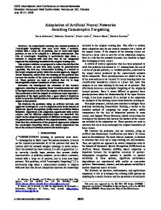
niŽcant temporal changes in the interactions among neurons in both the direction and the strength of the coupling, (2) the average coupling strength over the network of neurons appears to increase during the adaptation but return to the original level after adaptation, and (3) the connecting architecture of the network is typically altered after adaptation. Neural activities in the brain are undoubtedly nonlinear. Naturally, one might thus ask why we choose to focus on linear methods to address the learning and adaptation problem in M1. As for linear methods, nonlinear methods can also be classiŽed as nonparametric and parametric. A popular class of nonparametric method is nonlinear time-series analysis based on the time-delay embedding techniques (Takens, 1981; Sauer, Yorke, & Casdagli, 1991, 1997; Sauer, 1994, 1995; Castro & Sauer, 1997), which can yield meaningful information for dynamical systems of low dimensionality (Sauer et al., 1997) and for relatively noiseless data over a long time span. However, for the task that we face, all these assumptions are violated. Parametric methods, on the other hand, utilize nonlinear models such as artiŽcial neural networks and fuzzy logic schemes to identify the underlying nonlinear system and estimate the interactions between neurons, which are promising but largely empirical and generally more difŽcult to deal with than linear methods. Our philosophy is that given a set of neural data, which are typically noisy and short, the linear method should be considered Žrst, at least for the purpose of gaining insights. Often such an exploration can lead to meaningful results. Indeed, as we will demonstrate in this article, by carefully preprocessing the input data and selecting model parameters, the MVAR/DTF approach can yield a large amount of information that can help us better understand the functional changes in neural interactions during learning and adaptation. 2 Material and Methods 2.1 Behavioral Experiments and Data Collection. The Institutional Animal Care and Use Committee at Arizona State University approved the behavioral paradigm, surgical procedures, and general animal care. The guidelines suggested by the Association for Assessment and Accreditation of Laboratory Animal Care and the Society for Neuroscience were followed. The experimental subject is a rhesus monkey trained to perform behavioral movements in a three-dimensional space, similar to the standard center-out tasks in motor cortical studies (Georgopoulos, Kalaska, Caminiti, & Massy, 1982; Schwartz, Kettner, & Georgopoulos, 1988; Georgopoulos, Kettner, & Schwartz, 1988). In our experiment, eight targets with lights and push buttons are located at the vertices of a 13 cm cube as shown in Figure 1A (He, Weber, & Cai, 2002). In the center of the cube is an additional target. Each trial begins with the illumination of the central target (center on). The monkey is trained to push and hold the button on the central target until a randomly selected target at a vertex is illuminated, at which time

2362

L. Zhu, Y. Lai, F. Hoppensteadt, and J. He

the monkey is supposed to reach out to the new target. A successful trial requires that the monkey reach the vertex target and push the button in time less than 600 ms and hold it at least 100 ms. The coordinates of hand trajectories were recorded by using a 3D optoelectronic motion analysis system (Optotrak System, Northern Digital). To test the monkey’s abilities to learn and to adapt, perturbations at the behavioral level are applied to disturb the monkey’s already well-trained reaching-out movement. To apply the perturbation, the monkey’s wrist was attached to a pneumatic cylinder through a string. A brief (75 ms) pulling force, produced by the pneumatic cylinder, is delivered through the string after the hand moved about 2 cm from the center target. The approximate direction of the pulling force for each target is shown in Figure 1A. To assess the neural behavior in M1, two 16-channel arrays of microelectrodes are chronically implanted in the precentral arm area. Extracellular potentials are recorded on a 96-channel Multi-channel Acquisition Processor (MAP, Plexon, Inc., Dallas, TX). The MAP can isolate up to four units on a single electrode by using waveform discrimination. Spike times from all active channels are recorded along with behavioral event times (e.g., the center-release time), which allow us to separate the behavioral task periods. The waveform samples (800 ¹s clip) of action potentials were also recorded throughout the experiment to verify the stability of the neural recordings across multiple days. Further details are given in Weber (2001) and He, Weber, and Cai (2002). Before the surgery, the monkey was trained to be able to perform unperturbed trials successfully, without the string attached. Then electrodes were implanted. After a one-week period of postsurgical recovery, the monkey was attached to the string during all experiments, no matter whether the perturbation was applied. The experiments began with four-week unperturbed trials. The average trajectory on the last day of unperturbed trials is shown in Figure 1B (the trajectory with 0). From day 1 on, the perturbation force began to be applied. At the beginning, the perturbation force tended to signiŽcantly displace the monkey’s arm motion from its normal, unperturbed trajectory. After about one week, the monkey is able to compensate for the perturbation in a fairly predictable way (He et al., 2002), which can be seen by comparing the trajectories on days 1 and 8 in Figure 1B. 2.2 MVAR Model and Its Validity. Our analysis is based on MVAR modeling. Suppose the multichannel time series X.n/ D [x1 .n/; x2 .n/; : : : ; xM .n/]T are generated from a stochastic system or a deterministic system of high dimensionality under the inuence of strong noise, where n is the discrete time. The current state is determined by the linear combination of K previous states and uncorrelated white noise N.n/ D [n1 .n/; n2 .n/; : : : ; nM .n/]T if the time span between the previous and current states is not too large (otherwise, they may become uncorrelated). In MVAR modeling, X.n/

Probing Changes in Neural Interaction During Adaptation (A )

4

2

5

(C )

(B)

7

2363

0 0 1

16

8

3 6

(D) Neuron 1

­4

8

1 Perturbation Direction 40

16 ­3

15

40

(F) Neuron 3

(E) Neuron 2

Firing Rate (spikes/sec)

40 20 0

20

(G) Neuron 4

0

20 (H) Neuron 5

0

40

40

40

20

20

20

0 ­5

0

5

10 15

0 ­5

0 5 10 15 Adaptation Days

0 ­5

(I) Neuron 6

0

5

10 15

Figure 1: (A) Targets and perturbation force Želd in front of the monkey. The eight targets are located at the vertices of a 13 cm cube. (B–C) The hand trajectories toward target 4 (top left). The digits indicate the experiment date (e.g., 1 indicates the Žrst day of perturbed trials). Each trajectory shown here is averaged over all the trials during one day. The thick curves correspond to perturbed trials, and the thin curves correspond to unperturbed trials. (D–I) The changes of Žring rates from six neurons (set 1) in M1 across the adaptation days. The Žring rates are averaged over trials on target 4 during the period from target-on to center-release.

is written as X.n/ D

K X lD1

A.l/ ¢ X.n ¡ l/ C N.n/;

(2.1)

where A.l/’s (l D 1; : : : ; K) are M£M coefŽcient matrices, the noisy vector N.n/ characterizes the modeling error, and K is the model order. The Akaike’s Žnal prediction error (FPE) criterion (Akaike, 1974) can be used to determine the optimal model order. Equation 2.1 is a linear model, and, hence, it can represent linear, stochastic systems for suitable choice of K. While the underlying dynamical system generating the observed neural activities is undoubtedly nonlinear (Free-

2364

L. Zhu, Y. Lai, F. Hoppensteadt, and J. He

man, 1985, 1987; Freeman & Skarda, 1985), its dimensionality may be so high that effectively, it cannot be distinguished from a linear stochastic process (Lai, Osorio, Harrison, & Frei, 2002). Our central hypothesis is then that the neural dynamics of the brain can be described practically by linear stochastic models such as equation 2.1. Stationarity of the stochastic process is another issue of concern. Notice that the MVAR model deŽned by equation 2.1 is time invariant, which requires that the time series X.n/ be stationary, with each channel of X.n/ stationary and all channels jointly stationary. However, in our experiment, during the reaching-out movement, the monkey’s brain performs a cognitive task; thus, the state of the brain may change rapidly in time, which results in changes in the Žring rate and Žring pattern of the neurons and likely changes in the functional interactions between neurons as well. In reality, neural recordings are thus nonstationary. While the stationarity of recording from individual channel may be improved by subtracting its mean and dividing by the standard deviation for each point in the time series, computationally it is hard to improve the joint stationarity. Nonetheless, if the interactions among neurons are approximately invariant or slowly varying over a short time period on which the analysis is focused, the neural interactions can be assumed to be approximately time invariant. For this reason, in what follows, we focus only on the short time period from target-on to center-release (300 ms on average). Investigation on another period, from center-release to target-hit, yields similar results. 2.3 Dealing with Short, Sparse Spike Trains. For nonstationary, continuous-time signals, it is necessary to preprocess the data to reduce the inuence of nonstationarity, such as dividing the data into a set of short but relatively stationary segments or removing the time-varying average from the data. In situations where only short time series are available, MVAR modeling requires an ensemble of such data sets to yield a stable MVAR model. Our neural recordings are even worse than merely being short because they are not continuous-time signals but spike trains, which can be regarded as being from a point process. That is, the recorded information is a set of ordered times at which spikes occur, as follows: t 0 < t1 < t2 < ¢ ¢ ¢ < tn < ¢ ¢ ¢ In order to apply a multivariate time-series analysis, it is necessary to convert the sequence of times into a continuous-time waveform (Brillinger, 1978). A standard technique is to construct x.t/ D

X n

±.t ¡ tn /

(2.2)

and then pass x.t/ through a low-pass Žlter or to convolve x.t/ with a kernel function to remove high-frequency components (Sameshima & Baccala,

Probing Changes in Neural Interaction During Adaptation

2365

1999; Kaminski ´ et al., 2001), generating a continuous-time signal more suitable for MVAR modeling and also capable of capturing the phase information of the spike train. With appropriate adjustments of parameters (e.g., the cutoff frequency of low-pass Žlter), such preprocessing can be quite useful if the spike train contains a large number of spikes and the recordings are relatively stationary. If the spikes are sparse, the cutoff frequency of the lowpass Žlter has to be very low, resulting in the response delay of the low-pass Žlter comparable to the duration of the spike train. In this situation, part of the phase information of the spike train will be lost in the output signal, and great effort is needed to compensate the distorted phase information. The neural data from our experiments are only a sparse set of spikes; the number is typically so small that the standard preprocessing method becomes unsuitable. Here we propose a general method of preprocessing short, sparse spike trains so that MVAR modeling can be applied. We note that for multichannel spike trains, the relative phase, or the relative timing of spikes among different channels, is the only information from which neural interactions may be extracted. Our basic idea is to convert a spike train into continuous-time signals of instantaneous Žring rate, which should preserve the phase information. As such, the rate proŽle and the original spike train code the same temporal Žring behavior of the neuron. Consider, for example, integrate-and-Žre neurons. If the Žring threshold is known, the instantaneous Žring rate can be converted into the spike train, and vice versa, without loss of information. Our procedure to construct a continuous-time rate function from a spike train consists of three steps, as illustrated in Figures 2A through 2C. Fluctuations of the resulting instantaneous Žring rate reect the irregularity in the occurrences of spikes, so a coherence measure between two instantaneous Žring-rate signals can yield information about the interactions between the two neurons. The temporal property of the rate signal obtained this way lies somewhere between those of the mean rate and the original spike train, with ±T as the parameter for adjusting the relative weights of the two. We investigate the inuence of the value of ±T on the modeling error by utilizing a neural network model with a known network structure (see section 3). We Žnd, empirically, that varying ±T, insofar as it is smaller than the mean interspike interval T, will generally not affect the result. Experiments under situations with different Žring rates suggest that choosing ±T to be a fraction of T (say, T=4) is proper in the sense that the estimate of the network structure is correct. 2.4 Directed Transfer Function and Coupling Strength Measurement. Since the instantaneous rate proŽle can be regarded as a continuous-time signal, multivariate time-series analysis techniques can be applied readily. Performing a Fourier transform of equation 2.1 yields X. f / D A¡1 . f / ¢ N. f / ´ H. f / ¢ N. f /:

(2.3)

2366

L. Zhu, Y. Lai, F. Hoppensteadt, and J. He

f(n=i) 1

­ t1

(A)

t1

t2 1 ­ t2

t

dT (B) f(n)

i

n

(C) n Figure 2: Construction of a continuous-time rate signal from a spike train. (A) The original spike train. The averaged Žring rate during each interspike interval (e.g., ¿1 ) is taken to be the inverse of the interval (e.g., 1=¿1 ). (B) Forming a time series with sampling period ±T, where f .n D i/ is the area of shaded region in (A). (C) The resulting continuous-time rate signal, after low-pass Žltering (FIR with cutoff frequency equal to 0.2 of Nyquist frequency).

The DTF from the ith channel to the jth channel is deŽned as (Kaminski ´ & Blinowska, 1991) jHji . f /j2 DTF. f /ji D P M : 2 mD1 jHjm . f /j

(2.4)

From a numerical example shown in Figures 3D and 3E, we see that a convenient quantity to characterize the direct interactions among neurons is Z 1 DTFji . f / df; (2.5) Cji D 0

which is the total area under the transfer function and can be regarded as being proportional to the “energy” transfer, or the direct coupling strength, from neuron i to neuron j. Equivalently, one can make use of the coefŽcient matrices A.l/ in the time domain to compute the direct coupling strength (Kaminski ´ et al., 2001), as follows: PK 2 lD1 Aji .l/ (2.6) Cji D P M P K ; 2 j;iD1 lD1 Aji .l/ where 0 · Cji · 1.

Probing Changes in Neural Interaction During Adaptation

2367

Figure 3: A numerical network model of Žve interacting Hodgkin-Huxley neurons. (see section 3 for details). There are Žve neurons—one isolated and four connected with coupling strength k—driven by Žve independent external stimuli Ii ’s. A typical set of action potentials from Žve neurons with k D 2 is shown in C. The mutual interactions among neurons 2 and 3 are explicitly reected by the values of the DTFs in D and E. The estimated coupling architecture of the network with signiŽcant interactions is shown in B, where 100 trials with k D 2 and the signiŽcance level ® D 0:05 are used. The arrows indicate the directions of coupling, and the thickness of lines signiŽes the relative coupling strength.

2368

L. Zhu, Y. Lai, F. Hoppensteadt, and J. He

The above deŽnition of the coupling strength Cji is meaningful only in the statistical sense, since Aji in equation 2.6 is estimated from the input data. To test whether the computed values of the coupling strengths are statistically signiŽcant, it is necessary to conduct a null-hypothesis test. In this regard, the method of surrogate data (Theiler, Eubank, Longtin, Galdrikian, & Farmer, 1992; Kaminski ´ et al., 2001) is convenient. For a set of given time series, its surrogate is generated by randomly shufing the sampling points of each channel independently so that any functional interactions among them are destroyed while the energy of the original signals is maintained. Then the distribution of the coupling strength measurement, F.x/ D Probability.C > x/, can be empirically obtained by using a large number of independently shufed surrogate data sets. For a given signiŽcance level ® (D 0:05 used in this study), the causal inuence from channel i to j is said to be signiŽcant if F.Cji / < ®. One of the advantages of multivariate modeling over pairwise time-series analysis is that a more accurate estimate on causal interaction can be made by taking the inuence of other channels into account. Consider a situation where two neurons are driven by a common neuron. In this case, a pairwise method may suggest that there is an interaction between the two driven neurons since they are correlated. However, as we will show in section 3, if an MVAR model is Žtted into the measurements of all three neurons, direct interaction between the two driven neurons may not pass the signiŽcance test, and correct estimation of the connection structure of this three-neuron network can be made. It should be noted that multivariate analysis cannot distinguish between direct or indirect interaction as with pairwise methods if the common input is not included in the MVAR model. Nevertheless, multivariate methods are preferred if multichannel measurements are available. 3 Results To gain conŽdence on the applicability of our procedure to realistic neural recordings, we Žrst study a small artiŽcial neural network consisting of Žve interacting, Hodgkin-Huxley-type neurons, as shown in Figure 3. 3.1 Benchmark Testing Using a Model Network of Hodgkin-HuxleyType Neurons. In this network, each neuron is modeled by the following set of ordinary differential equations (Wilson, 1999): dV D ¡.17:81 C 47:58V C 33:8V2 /.V ¡ 0:48/ dt ¡26R.V C 0:95/ C I ¡ kgV 1 dR D [¡R C 1:29V C 0:79 C 3:3.V C 0:38/2 ]; 5:6 dt

(3.1)

Probing Changes in Neural Interaction During Adaptation

2369

1 df D [¡ f C Sgn.Vpre C 0:2/]; dt ¿syn 1 dg D .¡g C f /; dt ¿syn where Sgn.x/ is the sign function, V is the membrane potential, R is the recovery variable, and f is an intermediate variable for the synaptic potential g. The Žrst two equations characterize the dynamics of the membrane potential, which are a simpliŽed version of the Hodgkin-Huxley equations for mammalian cortical neurons, and I is the sum of external stimuli, excluding the one from the presynaptic neuron. Independent bandpass random noise is used to mimic external stimuli for different neurons. The last two equations govern the dynamics of the synaptic potential. All synapses in the network have the same coupling strength k and time constant ¿syn D 2 ms. Briey, the membrane potential Vpre of presynaptic neuron is coupled to postsynaptic neuron, V, through an excitatory synapse with time constant ¿syn. Figure 3C shows the action potentials from the Žve neurons with k D 2 during one trial. On average, each neuron Žres about 16 to 30 spikes during this short period. We utilize our procedure based on the instantaneous Žring rate to convert the spike trains into continuous-time signals. The same procedure is performed for 100 independent trials. In order to improve the stationarity, the ensemble mean over 100 trials is subtracted, and the data set is divided by the standard deviation. A MVAR model is Žt to the resulting data. The FPE criterion gives the optimal model order of eight. Utilizing the procedure in equation 2.6, we obtain the coupling-strength matrix C. Similarly, we can obtain coupling strength matrix CS from a surrogate data set. For the null hypothesis test, we repeat this process many times and obtain the empirical distribution of coupling strength measurement CjiS for each connection. The Žnal estimation of the network coupling architecture is shown in Figure 3B. As expected, neuron 5 is isolated from the rest of the network; neurons 1 and 2 are bidirectionally coupled; and there is no direct interaction between neurons 3 and 4, which are driven by neuron 2. The simulation indicates the presence of a small amount of coupling from neurons 4 to 2, which contradicts the network conŽguration. This small amount of energy “leakage” is induced by the error of modeling and may increase as the real coupling strength increases. However, considering the fact that this energy leakage occupies only a very small portion of the total coupling energy (less than 5% in this example), we regard the result as agreeing with the original network architecture reasonably well. Figures 4A through 4H show how the coupling strength measure Cji of each connection changes as the actual coupling strength k is increased from 1 to 4. The estimated coupling strength apparently reects these changes. We also see that the

2370

L. Zhu, Y. Lai, F. Hoppensteadt, and J. He

0.2

(A) 2­ >1

0.1

(B) 1­ >2

0.1

0.1

0.05

0.05

0

0

0

0.1

(D) 2­ >3

0.1

(E) 4­ >2

0.1

0.05

0.05

0.05

0

0

0

0.1

(G) 5­ >4

0.1

(C) 3­ >2

(F) 2­ >4

(I) S C

(H) 4­ >5 0.4

0.05 0 1

0.05

2

3

4

0 1

0.2

2

k

3

4

0 1

2

3

4

Figure 4: (A–H) Estimated coupling strength of individual connections versus the actual coupling strength k. (I) Coupling strength level averaged over the entire network, 6C, versus the assumed coupling k.

estimated coupling strengths do not grow linearly with the true coupling strength, and the growth rates for different connections are different. This is due to the fact that the underling system, equation 3.1, is nonlinear. A measurement on the output of the system may have a very complicated nonlinear functional relation with system parameters. Nevertheless, since the function of the coupling strength measurement versus k, C D f .k/, has a monotonic behavior, the changes of C can actually reect the changes of true coupling strength k. Thus, when we investigate the changes of k from data, we will focus on the changes of C without attempting to Žnd the function f . While Cji gives the strength of individual connections, the summation of Cji , 6C, gives the estimation of the coupling-strength level of the whole network. Figure 4I shows that 6C increases with k, indicating that our procedure can detect the change in neural interactions correctly. 3.2 Analysis of Neural Recordings from M1 During Adaptation. In our experiments with monkey, the session each day typically lasts for about 2 hours; around 80 trials were performed for each target. During the experi-

Probing Changes in Neural Interaction During Adaptation

2371

ments, the same population of active neurons (about 30 to 50) was recorded simultaneously. A total of 44 M1 neurons were considered for this study. For each trial, we analyze the neuronal activity during the period from target-on to center-release. The typical patterns of changes in Žring rates are shown in Figures 1D through 1I, which were obtained from the responses toward target 4. It also appears that the changing patterns on different targets are similar for the same neuron during the adaptation. Among the 44 neurons, the Žring rates of about 36%.16=44/ of neurons were found to be fairly constant during preadaptation days, while the ones of the others were not. During the adaptation, the Žring rates of about 18%.8=44/ of neurons were found to have increased; 30%.14=44/ increased Žrst and then dropped back; 11%.5=44/ decreased; 11%.5=44/ decreased, increased, and then dropped back; and 27%.12=44/ did not show any clear trend. We are interested in how neural interactions evolve during adaptation. Among the 44 neurons, some appear to be relatively more active (e.g., Žring more than 20 spikes in one trial). For statistical reliability, we select 17 active neurons and group them into three sets for the purpose of cross validation. The Žrst set consists of six neurons, which Žre actively throughout the experimental period. The changes of their Žring rates are shown in Figures 1D through 1I. The second set consists of eight neurons (four are also in the Žrst set), which also Žre actively through the experiments of all days. The third set varies on different days and consists of eight neurons, which Žre most actively on each day. For each set on each day, the recorded spike trains are Žrst preprocessed. The resulting data are then used to construct an MVAR model, and the coupling matrices are computed. Null hypothesis tests are performed to Žnd statistically signiŽcant connections, based on the empirical distributions obtained from the surrogate data. Figures 5A through 5C show the changes of interactions between the neurons in the Žrst set during the preadaptation days. It is not surprising to see that the connection structure between these neurons appears not quite stationary, since the monkey’s hand trajectories and the activities of single neurons were not stationary either in the preadaptation days, as shown in Figure 1. Despite the presence of these nonstationarities, consistency can still be observed (e.g., the forward connection from neuron 6 to 5). During the adaptation, as shown in Figures 5D through 5H, consistent connections clearly appeared (e.g., the one between neurons 3 and 5). It is also evident from Figures 5A through 5H that the directions of neural interactions tend to change during the adaptation, and the coupling strength of neural interactions can uctuate as well. These observations provide direct evidence that adaptation is accompanied by synaptic modiŽcation, which may occur rather quickly. A question is whether the synaptic modiŽcation during adaptation tends to modify the connecting architecture of the neural network, established during the learning process in unperturbed trials, only slightly or to change the architecture totally (i.e., reorganization of the interaction paths). Fig-

2372

L. Zhu, Y. Lai, F. Hoppensteadt, and J. He

Figure 5: Results obtained from a set of six neurons on trials with target 4. (A–H) Estimated network structure on different days. The thickness of lines signiŽes the relative coupling strength. (I) All possible connections between these six neurons by superposing the results from 14 days. Their strengths are ignored.

ures 5A through 5H show the architectures of the six-neuron network on different days during adaptation for target 4. We see that on the timescale of days, adaptation tends to change the interacting architecture within the network in a substantial manner, suggesting that the internal network of neurons in M1 is very exible. It is thus likely that the strategy employed by the brain for adaptation in response to external perturbations is to reorganize the neural network. If there exist extensive physical connections (synapses) among neurons in M1, reorganization can be achieved by changing the existing synaptic connections rather than growing new synapses. It has been shown that this reorganization can have a very rapid time course (within a few hours) (Jacobs & Donoghue, 1991). As shown in Figure 5I,

Probing Changes in Neural Interaction During Adaptation

(A) Target 1

(B) Target 2

1

4

0.5

2

SC

0

0

(C) Target 3

4

2

2

1

0

0

(E) Target 5

2

2

1

1

0

0

(G) Target 7

1.5

1.5

1

1

0.5

0.5

0 ­5

0

5

10

2373

15

0 ­5

(D) Target 4

(F) Target 6

(H) Target 8

0

5

10

15

Adaptation Days Figure 6: Estimated coupling strength level across adaptation days. Results are obtained from 17 neurons.

over the period of interest (less than three weeks), direct or indirect connections can be established among almost any two neurons. Studies on different targets and different neuron sets also support the above Žndings. The overall changes of interaction level among these 17 neurons are shown in Figure 6, estimated by averaging the results from the above three sets. The general observations are the following:

2374

L. Zhu, Y. Lai, F. Hoppensteadt, and J. He

² The estimated level of neural interaction strength still changes without showing any clear trend (increasing or decreasing) during the last three days of the four-week training on unperturbed trials with string attached. This uctuation may simply come from the uncertainty of the coupling strength estimation. However, considering the consistency presenting in Figures 5A through 5H and the continuity presenting in Figure 6 during adaptation (e.g., Figure 6G after day 9), we believe that this uctuation does not come from the estimate uncertainty, but it reects the changes of real interaction levels. The observations of hand trajectory and Žring rate of single neuron also support this argument. As shown in Figure 1, the trajectories and Žring rates on days ¡4, ¡3, and 0 are considerably different. One possible reason is that without the guidance of external force, the reaching-out movements were relatively random (or “noisy”) due to the nature of the neuronal Žring and muscle contraction, even after a relatively long period of training. However, after being exposed to the external force, it developed a guided trajectory to compensate the perturbation, which can be seen from the changes of trajectories on days 1, 8, and 15 in Figure 1B. ² A signiŽcant increase on interaction level appears at the beginning of the second adaptation week after a two-day break. This observation indicates that the process of memorization plays an important role during learning and adaptation. ² After another week’s adaptation, the overall coupling level returns to the same level as before the adaptation. Although the details of changes on interaction levels are different for different targets, the restoration of the coupling strengths after adaptation appears to be the rule governing the change in neural interactions during adaptation. Learning and adaptation in general may involve many neurons in M1 and in other regions of the brain as well. Since the neurons from which spike trains are recorded are randomly selected, the 17 active neurons utilized in our analysis may constitute a reasonably representative set of the entire population of the involved neurons in M1. 4 Discussion In this study, we presented an algorithm based on MVAR models and DTFs to probe the functional interactions among neurons by using multichannel neural recordings (spike trains). In order to make the algorithm applicable for situations where the spike trains are short and sparse, a procedure is proposed to preprocess the data by converting the spike trains into instantaneous Žring rates. A statistical test based on surrogate data is used to evaluate the signiŽcance of the coupling strength measurements. The behavior of this algorithm was examined by using both simulated data and actual neural recordings. Our study on the simulated network of Hodgkin-Huxley

Probing Changes in Neural Interaction During Adaptation

2375

neurons shows that despite minor errors in estimations, the algorithm is capable of yielding the strengths of functional interactions among neurons and the sensitivity to the changes of these interaction strengths. These indicate that our algorithm may be a useful tool to characterize the interaction among neurons, which is important for investigating how the brain learns and adapts. We analyzed spike trains generated by neurons in M1 from a monkey during reaching-out movements in controlled experiments. Although the results presented here are only preliminary, the analysis based on our algorithm provides evidence that the process of learning and adaptation tends to cause changes in the neural network in two ways. First, during the learning and adaptation, the synaptic strengths (or the coupling strengths) among neurons change, and thus new dynamics takes over in the network of neurons. At the beginning of adaptation, the interactions among neurons tend to be strengthened. One possible result of stronger coupling strength among the neurons in a network is faster response for the whole network to input stimulus. The expense, however, is more energy consumption due to the increased coupling and thus the increased metabolic activity of the brain. After adaptation, the coupling strengths among neurons return to the original level, which means less energy consumption for performing the task. Second, the connecting architecture of the neural network tends to change signiŽcantly as a result of learning and adaptation. Perhaps, to achieve fast response, changing the architecture may be better than increasing the coupling strength. It is possible that this learning process never stops, and overtraining can always change the interactions among neurons. Our study also indicates that both good performance and energy efŽciency are the goals of the adaptation. While the goal of good performance was enforced by food reward to the monkey, the goal of energy efŽciency is achieved by the nature of the learning mechanism of the brain. Acknowledgments This work is sponsored by DARPA under Grant No. MDA972-00-1-0027. References Akaike, H. (1974). A new look at the statistical model identiŽcation. IEEE Trans. Auto. Control, 19, 716–723. Bressler, S. L., Coppola, R., & Nakamura, R. (1993). Episodic multiregional cortical coherence at multiple frequencies during visual task performance. Nature, 366, 153–156. Brillinger, D. R. (1978). Comparative aspects of the study of ordinary time series and point processes. Developments in Statistics, 5, 33–133. Castro, R. & Sauer, T. (1997). Correlation dimension of attractors through interspike intervals. Phys. Rev. E, 55, 287–290.

2376

L. Zhu, Y. Lai, F. Hoppensteadt, and J. He

Ding, M., Bressler, S. L., Yang, W., & Liang, H. (2000). Short-window spectral analysis of cortical event-related potentials by adaptive multivariate autoregressive modeling: Data preprocessing, model validation, and variability assessment. Biol. Cybern., 83, 35–45. Duckrow, R. B., & Spercer, S. S. (1992). Regional coherence and the transer of ictal activity during seizure onset in the medial temporal lobe. Electroenceph. Clin. Neurophysiol., 82, 415–422. Florence, S. L., & Kaas, J. H. (1995). Large-scale reorganization at multiple levels of the somatosensory pathway follows therapeutic amputation of the hand in monkeys. J. Neurosci., 15, 8083–8095. Freeman, W. J. (1985). The EEG with nonlinear dynamics. Electroen. Clin. Neuro., 61, S224. Freeman, W. J. (1987). Brains make chaos to make sense of the world. Behav. Brain Sci., 10, 161–173. Freeman, W. J., & Skarda, C. A. (1985). Spatial EEG patterns, nonlinear dynamics and perception—the neo-Sherringtonian view. Brain Res. Rev., 10, 147–175. Freiwald, W. A., Valdes, P., Bosch, J., Biscay, R., Jimenez, J. C., Rodriguez, L. M., Rodriguez, V., Kreiter, A. K., & Singer, W. (1999). Testing non-linearity and directedness of interactions between neural groups in the macaque inferotemporal cortex. J. Neurosci. Methods, 94, 105–119. Georgopoulos, A., Kalaska, J., Caminiti, R., & Massy, J. (1982). On the relations between the direction of two-dimensional arm movements and cell discharge in primate motor cortex. J. Neurosci., 2, 1527–1537. Georgopoulos, A., Kettner, R., & Schwartz, A. (1988). Primate motor cortex and free arm movements to visual targets in three-dimensional space. II. Coding of the direction of movement by a neuronal population. J. Neurosci., 8, 2928– 2937. Gersch, W. (1970). Spectral analysis of EEG’s by autoregressive decomposition of time series. Math Biosci., 7, 205–222. Gochin, P. M., Miller, E. K., Gross, C. G., & Gerstein, G. L. (1991). Functional interactions among neurons in inferior temporal cortex of the awake macaque. Exp. Brain Res., 84, 505–516. Granger, C. W. J. (1969). Investigating causal relations by econometric models and cross-spectral methods. Econometrica, 37, 424–438. He, J., Weber, D. J., & Cai, X. (2002). Adaptation in cortical control of arm movement. In Proceedings of the IFAC Congress. Barcelona. Ito, M. (2000). Mechanisms of motor learning in the cerebellum. Brain Res., 886, 237–245. Jacobs, K. M., & Donoghue, J. P. (1991). Reshaping the cortical motor map by unmasking latent intracortical connections. Science, 251, 944–947. Kaminski, ´ M. J., & Blinowska, K. J. (1991). A new method of the description of the information ow in the brain structures. Biol. Cybern., 65, 203–210. Kaminski, ´ M., Ding, M., Truccolo, W. A., & Bressler, S. L. (2001). Evaluating causal relations in neural systems: Granger causality, directed transfer function and statistical assessment of signiŽcance. Bio. Cybern., 85, 145–157. Karni, A., Meyer, G., Jezzard, P., Adams, M. M., Turner, R., & Ungerleider, L. G. (1995). Functional MRI evdence for adult motor cortex plasticity during motor skill learning. Nature, 377, 155–158.

Probing Changes in Neural Interaction During Adaptation

2377

Lai, Y.-C., Osorio, I., Harrison, M. A. F., & Frei, M. (2002). Correlation-dimension and autocorrelation uctuations in epileptic seizure dynamics. Phys. Rev. E, 65, 031921(1–5). Li, C.-S. R., Padoa-Schioppa, C., & Bizzi, E. (2001). Neuronal correlates of motor performance and motor learning in the primary motor cortex of monkeys adapting to an external force Želd. Neuron, 30, 593–607. Muller, J. R., Metha, A. B., Krauskopf, J., & Lennie, P. (1999). Rapid adaptation in visual cortex to the structure of images. Science, 287, 1405–1408. Nudo, R. J., Milliken, G. W., Jenkins, W. M., & Merzenich, M. M. (1996). Usedependent alterations of movement representations in primary motor cortex of adult squirrel monkeys. J. Neurosci., 16, 785–807. Pearson, K. G. (2000). Neural adaptation in the generation of rhythmic behavior. Annu. Rev. Physiol., 62, 723–753. Recanzone, G. H., Schreiner, C. E., & Merzenich, M. M. (1993). Plasticity in the frequency representation of primary auditory cortex following discrimination training in adult owl monkeys. J. Neurosci., 13, 87–103. Sameshima, K., & Baccala, L. A. (1999). Using partial directed coherence to describe neuronal ensemble interactions. J. Neurosci. Methods, 94, 93–103. Sanes, J. N., & Donoghue, J. P. (2000). Plasticity and primary motor cortex. Annu. Rev. Neurosci., 23, 393–415. Sauer, T. (1994). Reconstruction of dynamical systems from interspike intervals. Phys. Rev. Lett., 72, 3811–3814. Sauer, T. (1995). Interspike interval embedding of chaotic signals. Chaos, 5, 127– 132. Sauer, T., Yorke, J., & Casdagli, M. (1991). Embeddology. J. Stat. Phys., 65, 579– 616. Sauer, T., Yorke, J., & Casdagli, M. (1997). Nonlinear time series analysis. Cambridge: Cambridge University Press. Schwartz, A., Kettner, R., & Georgopoulos, A. (1988). Primate motor cortex and free arm movements to visual targets in three-dimensional space. I. Relations between single cell discharge and direction of movement. J. Neurosci., 8, 2913– 2927. Takens, F. (1981). Dynamical systems and turbulence. In D. Rand & L.-S. Young (Eds.), Lecture notes in mathematics (Vol. 898, pp. 366–381). Berlin: SpringerVerlag. Theiler, J., Eubank, S., Longtin, A., Galdrikian, B., & Farmer, J. D. (1992). Testing for nonlinearity in time series: The method of surrogate data. Physica D, 58, 77–94. Weber, D. J. (2001).Chronic, multi-electroderecordingsof cortical activityduring adaptation to repeated perturbations of reaching. Unpublished doctoral dissertation, Arizona State University, Tempe. Whittle, P. (1963). On the Žtting of multivariate autoregressions and the approximate factorization of a spectral matrix. Biometrika, 50, 129–134. Wilson, H. R. (1999). Spikes,decisions, and actions: The dynamical foundations of neuroscience. New York: Oxford University Press. Received July 16, 2002; accepted April 4, 2003.