Procedia Computer Science

Procedia Computer Science

Available online at www.sciencedirect.com

Procedia Computer Science 00 (2009) 000–000

www.elsevier.com/locate/procedia

International Conference on Computational Science, ICCS 2010

The Piecewise-Parabolic Boltzmann Advection Scheme (PPB) Applied to Multifluid Hydrodynamics Paul R. Woodward,a* David Portera, William Daib, Tyler Fuchsa, Tony Nowatzkia, Michael Knoxa, Guy Dimonteb, Falk Herwigb, and Chris Fryerb a

Laboratory for Computational Science & Engineering, University of Minnesota, 117 Pleasant St. S. E., Minneapolis, MN 55455, USA b Los Alamos National Laboratory, Los Alamos, New Mexico, USA

Abstract A new and powerful approach to multifluid hydrodynamics has been developed and applied over the last few years to a variety of problems involving the development of turbulent mixing of different fluids at unstable multifluid interfaces. As in the traditional volume of fluid techniques, a specially adapted advection scheme is applied within the context of a gas dynamics method, in this case the Piecewise-Parabolic Method (PPM). The multifluid fractional volume variable is advected using the PiecewiseParabolic Boltzmann (PPB) scheme, which is an extension to 3-D constrained advection of van Leer’s Scheme VI advection scheme for 1-D. Ten moments of the fractional volume in each grid cell are updated by PPB in a strictly conserving formulation. Unlike the recent Moment of Fluid method, which dates from around the same time as our initial work with PPB in PPM, we demand that if the fractional volume is non-vanishing anywhere in a grid cell, it must be so at all points inside the cell. This forces the representation of a sharp multifluid interface to be smeared out over at least one cell. Nevertheless, the subcell information maintained by the scheme, plus judicious handling of constraints that the fractional volume cannot be negative nor can it exceed unity, result in very sharp interface representations when this is appropriate. The advantages of this approach and the results it delivers on multiple applications are discussed.

Keywords: computational fluid dynamics, multifluid hydrodynamics, difference schemes for multifluid advection

1. Introduction During the last few years, our team at the University of Minnesota’s Laboratory for Computational Science & Engineering (LCSE) and at the Los Alamos National Laboratory (LANL) has been applying in our PPM computational fluid dynamics codes (cf. [1] and references therein) a new formulation of multifluid hydrodynamics that exploits the power of the moment-conserving Piecewise-Parabolic Boltzmann (PPB) advection scheme [2,3]. Although an officially released code module including the new scheme was generated in 2005 for the Los Alamos XRAGE code, the details of this new method have not been described in the literature. Here we briefly set out the basis of this new method and give results on two types of simulations that serve to illustrate its use in practical * Corresponding author. Tel.: 612-625-8049; fax: 612-626-0030. E-mail address: [email protected].

Author name / Procedia Computer Science 00 (2010) 000–000

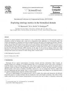
problems. Both examples involve advection dominated flows, and both involve unstable multifluid interfaces. The first, a study of the single-mode Rayleigh-Taylor instability, is acceleration driven, while the second, a study of entrainment of stably stratified fluid into a vigorous stellar interior convection zone, is shear driven. This work was begun in 2002 to address challenges in the treatment of multifluid interfaces in the RAGE code [4], and it has continued under LANL sponsorship as a means of addressing problems in turbulent multifluid mixing using LANL’s Roadrunner petaflop/s computing platform. The Rayleigh-Taylor problem we present here is an official test problem suggested by Dimonte for the IWPCTM-11 workshop in July of 2008 [5,6]. This should permit easy comparison of the results of our new method with those of other approaches. The second stellar convection problem is more computationally challenging. Its results are presented here as an illustration of the extent to which we can push the present technique in very demanding problems. This effort is an outgrowth of experience in the early 1990s using both the SLIC volume of fluid (VOF) method [7] in PPM and also using PPM’s internal method of contact discontinuity detection and steepening [8,9] in the study in 2-D of supersonic jets and shear layers in astrophysical contexts [10,11]. At that time, PPM’s internal treatment was preferred for most of our work in these application areas. However, both the PPM contact discontinuity steepener and the SLIC VOF technique are relatively crude by modern standards (see for example [12]). At the request of Mike Gittings and Bob Weaver at Los Alamos in 2002, we began to explore new multifluid interface capturing techniques and ultimately chose to exploit PPB’s carefully updated subcell information to give a better treatment for captured interfaces. Since the early 1990s, of course, VOF techniques have become very much elaborated and improved, with the innovations most closely related to our work being the recent development of the Moment of Fluid technique [13]. Our goal in developing PPB multifluid advection was simplicity and robustness for a capturing scheme targeted at handling multifluid gaseous problems, where the transition from a sharp to a smeared interface should be easily described and, ideally, not introduce glitches from sudden, relatively large changes in the numerical representation of the interface in a grid cell. VOF techniques are better adapted than PPB to the treatment of interfaces that are very sharp and must permanently remain so. With PPB we make a compromise. We are willing to give up some sharpness of an interface’s numerical representation in order to gain the robustness and simplicity of formulation that is a benefit of a continuous representation of the fractional volume variable. Our idea is that one is in any case limited in numerical computation by the unavoidable numerical diffusion resulting from the use of a grid. With PPB’s high-order, moment-conserving formulation, we keep this diffusion fairly small, and if it proves to be too large, our recommendation is to refine the grid, either locally, as in an AMR code, or globally, as we do in the problems reported here. Our PPM+PPB multifluid computation is fast, and modern computers are powerful, so that this recommended solution proves to be entirely practical for many problems of interest. 2. The moment-conserving approach originating with van Leer’s Scheme VI. In the mid 1970s, van Leer introduced his new approach to constrained numerical advection [14], which, along with Godunov’s idea of a numerical Riemann solver [15], was the foundation of the MUSCL [16] and PPM [17] schemes for gas dynamics. Van Leer’s Scheme VI [14] was a high-order extension of the ideas in MUSCL, and it was neither elaborated in 2- or 3-D nor was it given a method for applying monotonicity constraints. Scheme VI was extended to constrained 2-D advection in [2], and it is further simplified here (cf. [3]). The idea is that in each grid cell we provide independent information that is sufficient to define a unique interpolation function for the subcell distribution of a given advected variable, which we will call f, the fractional volume of a cell that is occupied by a given fluid. In 1D, Scheme VI uses the first three moments of f with a constant weighting function, corresponding to the idea that all points within the cell are equally important. These moments are f xk , defined as f xk , where the integration is over the full extent of the grid cell. We define these moments in terms of a coordinate x that is specific to the grid cell and that vanishes at its center and assumes the values ±1/2 at its edges. This formulation allows us to use 32-bit arithmetic, despite the 5th-order formal accuracy of the scheme in 1D. The means of updating these moments is straightforward. We simply determine from the moments for k = 0, 1, 2 the unique parabola that has these moments in the cell (see Figure 1). We then take the velocities at the leftand right-hand edges of the cell, averaged over the time step, and homologously stretch or squeeze the constrained parabola while translating it. This gives us a representation of the distribution of f at the end of the time step. Then


Figure 1. At the left, 3Eulerian grid cells are shown at the outset (top) of a 1-D pass and at the end of the pass (bottom). The interpolation parabolae determined by the 3 moments f , f x , and f x2 are indicated, with cross hatched areas indicating the portions that either move into adjacent cells during the time step or remain in the original cell. These same parabolae and cross hatched areas are shown at the bottom left in their final positions at the end of the 1-D pass. To obtain the new moments of f in the original Eulerian grid cell, we perform the integrals that define these moments over the cell (the region indicated by the bracket). At the right, alternative means of constraining interpolation parabolae are illustrated. At the top right, a parabola that has negative values is replaced by one blended with the cell average to the extent that its minimum value becomes zero. This process produces a slight diffusion and can leave a small positive region in front of an advancing multifluid interface, as shown in this example. At the bottom right, the same initial parabola is replaced by the unique parabola that assumes its minimum value at the right-hand edge of the cell. This replacement results in anti-diffusion and a slight steepening of the multifluid interface representation. Great care is taken in the numerical algorithm to make this second choice only when it is clearly justified by the initial data in this cell and in its 2 immediate neighbors.

we perform the integrals that define the moments, using these new distributions, to arrive at the new moments in the new grid cells. This procedure is described in detail in [2,3]. It is a straightforward matter to extend the method to 3D if we adopt a directional splitting approach, as we do in PPM. We then have 10 moments, f xkylzm , where 0 ≤ k + l + m ≤ 2 . We obtain a tremendous simplification by separately advecting in the x-pass the functions f , f y , f z , f y2, f y z , f z2. Not only is the advection of the higher-order functions following f in this list considerably simpler than the advection of f itself, but it is only to the advection of f that we need apply any constraints. This is an enormous benefit, since constraining the function in its full 3-D complexity would be a very difficult task indeed. This simple approach can be successful, because we get opportunities to constrain the terms in y and z in the y- and z-passes. It is important to note that in this process we omit several terms of high order that we judge to be unimportant. These express shear of the distribution of f in the y- and z-dimensions within the subcell distribution. Much experience shows that these terms are indeed quite unimportant, since we capture this effect at the scales above that of a single cell. These terms play a significant role in the flows we are concerned with only in thin shear layers and at the centers of vortices. In both of these cases, the diffusion introduced by omitting these terms is welcome. We wish to smear these regions out over a bit more than one grid cell width in any event in order to assure the robustness of the scheme. Our view is that if more resolution is required in these regions, then we should refine the grid. In [3], a method for handling these subcell shear terms is presented and results compared with the simpler scheme that ignores this aspect of the flow. The reader may judge from the results in [3] whether or not the extra complexity of handling subcell shear is worth its cost, which is about 2.5 times as much computation, but in our work we have decided that it is not. The method for constraining f by potentially resetting the values of

f x and f x2 is very important when


we use PPB advection to treat a multifluid fractional volume variable, as we do in this work. Experience has shown that one can very easily overdo the constraint function, and if this occurs, nearly all benefits of PPB advection over the much simpler and three times less expensive PPM advection are lost. As is shown through multiple examples in [3], we can roughly characterize the benefit of PPB over PPM advection by regarding it as equivalent to PPM advection on a grid refined by a factor of 3 in each dimension (and then, of course, also in time). One may wonder how this much greater accuracy of PPB over PPM can result, when both methods use parabolae for interpolation within grid cells. A likely explanation is that PPB operates upon 3 times as much independent information in each dimension as PPM, and it is therefore natural to expect it to deliver a result comparable to that which PPM would produce on a triply refined grid. However, it is very important to note that although PPB involves roughly 3 times the computational labor of PPM in updating each grid cell, to roughly equal its accuracy PPM would need to update 27 times as many grid cells with 3 times as many time steps. Thus PPB comes out ahead by about a factor of 27. The factor turns out to be a bit smaller than this in practice, because PPB involves less data reuse than PPM and consequently runs about 2 times slower in terms of Gflop/s. For the problems we will present here, we suggest that the benefit of PPB over PPM advection for the multifluid fractional volume is worth at least a grid refinement by a factor of 2, which translates into about a factor of 16 overall. For the advection of sharp multifluid interfaces, PPM’s contact discontinuity steepener is capable of generating a representation of the interface that is as thin as that resulting from PPB advection. The quality difference in these cases comes from the greater robustness of PPB interface representations, with far fewer numerical glitches and occasional pathological behaviors. The likely reason for this is the absence of “switches” in PPB between radically different treatments of the subcell distribution. If there are no switches, then they cannot go on or off unintentionally, and glitches are avoided. Here the means of avoidance is a smooth representation of the transition from one pure fluid to another on the grid. The high-order, momentconserving formulation of PPB enables it to maintain a sharp interface description that is nevertheless smooth. In Figure 1, we indicate the basic method of updating the moments of f in a grid cell in a 1-D pass. The process by which the unique parabola determined by the initial values of these moments in the cell is constrained is illustrated at the right in the figure. We employ one of two techniques to bring a parabola that assumes values less than 0 or greater than 1 into compliance: we either blend in enough of the constant function everywhere equal to the average value in the cell in order to bring the parabola into line, or we force the parabola to assume its extreme value at one edge of the cell or the other, with this extreme value reset to just satisfy the constraint. This second procedure is the monotonicity constraint procedure for PPM advection when we choose not to use its contact discontinuity detection and steepening algorithms. In PPB advection, we must apply the second procedure with extreme care, because it can fairly dramatically revise the distribution of the fluid within a cell. If this revision is not warranted, this procedure can destroy the very low rate of accumulation of error that is the main positive feature of PPB advection (cf. [14,2]). Therefore, in PPB advection, we never apply either constraint procedure simply to achieve monotone advection, since monotonicity is not a fundamental property of fluid behavior. The constraints are applied only to assure that the fractional volume assumes no physically impossible values inside the cell. We are careful never to move the extremum to a cell edge unless f in the neighbor cell next to that edge assumes that extreme value (to within a tiny tolerance, such as 2×10-6, which reflects the limitations of 32-bit floating point arithmetic). In such cases where our cell of interest has a neighbor cell containing only one pure fluid, we also reset the cell edge value of our interpolation parabola to this value (0 or 1), so that diffusion of the other fluid into this neighboring cell is minimized. The constraints that we have just described are both mild and very strongly motivated by the physics of the situation. They are consequently quite “safe,” and we see very few negative effects of these constraints in our multifluid simulations. On the contrary, we find that multifluid interfaces that we expect and wish to be sharp are indeed sharp in this approach. This is a surprise, because one would expect only steady diffusion to result from our smooth interface representation. In our simulations, we make literally hundreds of thousands of repetitions of the interpolation and advection procedure over the course of a single simulation, yet we observe that interface remain sharp when it is clear that they should do so. Our explanation for the absence of the expected interface diffusion is that multifluid interface instabilities cause the surface area of multifluid interfaces to increase, often without bound. This process, together with f being a constant of the motion, results in a simultaneous stretching and thinning of the interface, which causes it rapidly to assume the sharpest numerical representation our scheme allows. This sharpest permitted representation is indeed very sharp, as the examples below attest.


3. Incorporating PPB advection into PPM gas dynamics. In combining PPM gas dynamics with PPB advection for the multifluid fractional volume, f , we have followed the general procedure established by Roger DeBar’s original VOF method in the Kraken code from the 1960s [18]. The idea is that our picture of the grid cell’s internal state is that the fluids are in equilibrium with each other. DeBar assumed pressure equilibrium, but did not assume temperature equilibrium, which generally takes longer to establish. We will assume both, which makes our calculation much simpler. For gases, temperature equilibrium is a very reasonable assumption. To be consistent with our assumption of pressure equilibrium and our reluctance to explicitly handle subcell shear, we, like DeBar, assume that the fluids in a single cell all have a single velocity. For the Rayleigh-Taylor instability simulation of our first example below, revising this assumption could potentially improve the accuracy of the calculation. We describe the variation of the common pressure and velocity inside the cell with PPM-style parabolae (cf. [1] for the most recent procedure for obtaining these parabolae). In both pressure and temperature equilibrium, the ratio of the densities of two gases is determined by the ratio of their mean molecular weights, which is a global constant for the entire simulation if we neglect effects such as ionization that change the mean molecular weight. This means that if we are given the cell averages of the density of the mixture, ρ , and the fractional volume, f , of fluid B, we may derive the average densities, ρA and ρB , of the individual fluids. We may also derive an approximate value of γ for the mixture, such that the pressure, p, is given in terms of the internal energy, ε , of the mixture by the gamma-law equation of state: p = (γ – 1) ρ ε . A simple analysis results in the approximation: 1/ γ = fA / γA + fB / γB . Using this approximation for γ for the mixture, we may then also approximate the Eulerian sound speed, c, of the mixture by the usual formula: c2 = γp/ρ. Because both example problems that we will present here involve only weak compressibility effects and because of the limitation of space, we will not go into the manner in which strong shocks should be treated in this sort of multifluid formulation. For our problems, it is sufficient to handle the sound waves via the simple Riemann problem treatment described in [1] involving the fluid treated solely as a mixture. However, we take considerable care in handling the multifluid aspects of the advection terms in the governing fluid equations. Our Riemann problem solution at each grid cell interface follows the procedure described in detail in [1]. We base our Riemann problem upon left- and right-hand states derived from interpolation parabolae in the adjoining grid cells. We get away with interpolating only the pressure, p, and the x-velocity, ux , (in the x-pass) in order to produce estimates of the time-averaged pressures and x-velocities at the cell interfaces. Also, we do this by first interpolating the two sound-wave Riemann invariants (for waves moving in the x-direction) and then deriving the implied parabolae for p and ux. This procedure allows us to apply appropriate constraints to, first, the Riemann invariants and then, second, to the pressure and x-velocity. We apply no monotonicity constraints if an algorithm based upon cell averages in our cell and in its two neighbors on each side leads us to conclude that the functions are in fact smooth in this region. This round-about process is intended to give us interpolation parabolae for p and ux that are consistent with constrained parabolae for the two Riemann invariants. We use a similarly elaborated interpolation procedure for the individual fluid densities. First we determine parabolae for the differentials of the adiabatic invariants, as described in [1], for each fluid separately, and then from these and the pressure parabola we determine the implied density parabolae. This procedure may sound wasteful, but we have compared it with simpler procedures and find it worthwhile. The entire process is very fast on modern CPUs, for which floating point arithmetic is essentially free, given the far greater cost of accessing numbers stored in off-chip memory. For our example problems here, it is the computation of the fluxes associated with the Riemann invariants that move at the fluid velocity that poses the greatest challenge. We begin with the interpolation parabolae at the time of the beginning of the 1-D pass for f , the fractional volume for fluid B, and for ρA , ρB , uy , and uz . We use the time-averaged values of ux at the cell interfaces, obtained from the Riemann problem solution, to determine the time averaged velocity at each location within the grid cell by linear interpolation. We note that using this construction for the advection velocity in this 1-D pass causes our difference stencil to be one grid cell wider on each side of our cell of interest. This is therefore a costlier procedure in terms of the amount of data that we must communicate from node to node on a parallel computer than the original construction in PPM, but for our problems, which use large uniform grids, this cost is inconsequential. We compute the fluxes of the passively advected quantities listed above in two stages. First, we perform the elaborate update of the fractional volume, f , which


does not require knowledge of the advected amounts of the other quantities. This computation is performed as described earlier, and as depicted in Figure 1 (see [2,3] for details). We now use our interpolation parabolae for ρA and ρB to compute, separately, the advected masses of the two fluids. We then sum these to find the total advected mass. This procedure assures that we avoid interpolating across a multifluid interface any quantity like the density of the mixture, ρ, which would vary rapidly only because of the rapid variation of f. We have already described the variation of f with a highly accurate computation based upon independent subcell information. To obtain the variation of a quantity like ρ, we therefore expose its dependence upon f explicitly. We note that we can reasonably interpolate, for example, ρB , across the interface, because it is defined by our assumption of pressure and temperature equilibrium to have a reasonable value even in a cell on the side of the interface where f vanishes. In a similar fashion, we avoid interpolating the internal energy per unit mass of the mixture across a multifluid interface. This is proportional to p / ρ , and while p is only slowly varying across the interface, ρ varies rapidly due to the variation in f . Therefore we work with internal energy per unit volume, which we do even for a single fluid in our PPM scheme in order to account properly for contact discontinuities. We thus construct the flux of total energy for the mixture, dEL , at the left-hand cell interface as follows: Here we denote the left-hand cell interface by the subscript L and the time-average over the time step by an overbar. and denote the advected mass and advected volume (of the mixture), respectively. In applying the conservation laws, we must take care to maintain consistency with our moment-conserving computation in the PPB scheme for f . We will use the subscript N to denote the new time level and subscripts L and R for the left- and right-hand cell interfaces. For cell averages, we will drop our earlier use of angled brackets to make the equations more readable. We want to make sure that our new cell averages not only satisfy strict conservation, but we also want them to reflect our assumption of pressure and temperature equilibrium for the two fluids. Because our advection for f did not take this constraint into account, we may have to readjust f and, proportionately with that readjustment, all of its higher moments. We denote the differences of the mass fluxes for the individual fluids by , with a similar equation for fluid B. We use these flux differences to update the masses of the individual fluids in the cell. We may then define a mass flux difference that we would have if we were to replace all the fluid B with fluid A at the equilibrium density ratio, . We may now find our desired new value for ρA via , where V is the cell volume. The new density of fluid B in the cell, ρBN , is now obtained by multiplying ρAN by the equilibrium density ratio. It remains to determine the adjustment we need to make to the cell-averaged value f and, proportionally, to all its higher moments. This is easily done based upon our present knowledge of the new densities and mass fractions in the cell. Finally, we must obtain the new cellaveraged value of the pressure. We first recognize that pressure equilibrium in the new cell demands that . Using our previously computed fluxes of total energy and of x-, y-, and zmomentum, we increment the cell’s total energy and momenta. Using our updated value of the cell mass together with the new momenta and total energy, we get the new cell-averaged velocity components and total energy per unit mass. We now compute the new cell-averaged kinetic energy per unit mass, using the approximation that, for example, . Applying correction terms to this formula increases the size of the difference stencil, and we find it has little value except in turbulent regions of the flow, where we also find better ways to handle this issue through subgrid-scale turbulence models (see [19-21]). We do not use subgrid-scale turbulence models in the work reported here. At this point, after subtracting the new kinetic energy from the new total energy (per unit mass), we know together with and the ratio . This is sufficient information to obtain , because we must have . From , we may obtain the new cell-averaged pressure via the equation of state: . This completes the grid cell update for a 1-D pass. We perform 1-D passes in symmetrized sets of 6 using the same time step value. The order of the passes is xyzzyx, which limits us to second-order formal accuracy. As a means of eliminating the specialness, from a numerical point of view, of symmetry planes, for example, where one velocity component must always vanish, we perform our calculation in varying Galilean reference frames during each set of 12 1-D passes, for which we keep the time step value constant. At the outset of pass 1, we add a small x-velocity, , to every cell, accounting for


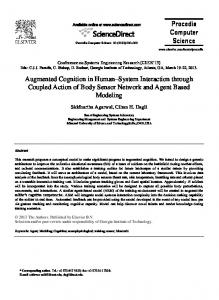
Figure 2. Four simulations of the same single-mode Rayleigh-Taylor instability problem are shown here using the PPB fractional volume advection in the PPM gas dynamics code, as described in the text. Each simulation begins with the same unperturbed state in a rectangular domain with a square horizontal cross section one length unit on a side. Periodic boundary conditions are enforced in the horizontal dimensions, and rigid walls are placed at the top and bottom. The gas in the unperturbed state is at rest and in hydrostatic equilibrium with a gravitational acceleration downward of amplitude g = 0.024. The gas has a gamma-law equation of state with γ = 5/3. At the midplane, the gas in the bottom half of the domain has density 1 and sound speed 1, so that our time unit is the sound crossing time of the domain in this gas at the midplane. In the top half of the domain, the gas is denser, with a density of 3 at the midplane. The initial unperturbed interface between the light and the heavy gases is represented by a smooth transition of the fractional volume, f , of the heavy fluid from 0 to 1 with a profile for and with δ = 0.05. This unperturbed initial multifluid interface is displaced by an amount, dy, given by for and with A = 0.01. The 4 runs differ in the values of the dynamic viscosity, µ, which is 10-5, 5×10-6, 2×10-6, and 0 going from left to right in the figure. Each simulation uses a uniform 3-D Cartesian grid with 512 cells across the horizontal width of the domain. These volume rendered images show the fractional volume, f , with values near 0 transparent and those near 1 a nearly transparent red. Mixtures that are more light than heavy fluid are blue, 50-50 mixtures are white, and those more heavy than light gas are yellow. Smooth rendering is possible despite a very thin interface representation, because f is provided for rendering at double the grid resolution, using the 10 independent moments updated by the code to generate 8 values per grid cell. As the viscosity is reduced, we first begin to see signs of the instability of the bubble and spike tips; Kelvin-Helmholtz instability due to the shear along the multifluid interface appears only as the viscosity is reduced still further. At later times, these secondary instabilities appear in all 4 of these simulations. The 4 flows are all shown at 30 sound crossing times of the periodic domain in the initial light fluid at the midplane.

the change in the total energy that this implies, and at the end of this pass we subtract this x-velocity again. In the . In pass seven and 12, both x-passes, we add x-velocities and . sixth pass, also an x-pass, we add We do a similar set of velocity adjustments in the other dimensions. This method of grid jiggling, which we apply only in the 2 horizontal dimensions in the Rayleigh-Taylor problems presented below, works very well with the jiggling velocity, set equal to 2.5% of the unperturbed speed of sound. We also find that results are not sensitive to the value we choose for . 4. Dimonte’s Single-Mode Rayleigh-Taylor Test Problem Over the last two years, we have applied our new multifluid PPM+PPB code to the study of turbulent mixing of multiple fluids driven by acceleration of multifluid interfaces. These studies have so far involved low Mach number flows driven by an effective gravity from an unstable initial configuration. The low Mach numbers together with our code’s explicit formulation mean that several time steps are required to move a multifluid interface across one grid cell width. If our method were prone to numerical diffusion of the interface, it would definitely show in these applications. Instead, the interfaces are remarkably sharp, as can be seen in the examples in Figure 2. At the same time, the single-mode test problem shown in Figure 2 gives ample opportunity, with its very fine grid, for the interface treatment to break down, produce unwanted glitches, etc. In the figure, a sequence of flow simulations with decreasing values of the Navier-Stokes dynamic viscosity, µ, is shown, so that the reader can form an independent


Figure 3. Volume visualizations of the mixing fraction of entrained hydrogen fuel (left) and vorticity magnitude (right) in the helium shell flash convection zone of an asymptotic giant branch (AGB) star of 2 solar masses. We have used the PPM gas dynamics code with PPB multifluid advection for the volume fraction of the stably stratified, relatively buoyant hydrogen/helium fuel above the convection zone. The uniform 3-D Cartesian grid has 5763 cells, containing the entire stellar core region out to a radius of 35,000 km. The flow is shown 5 simulated hours after heat from helium burning is injected at the base of the convection zone to initiate the convection from a static initial state adapted from a 1-D stellar evolution simulation of Herwig. Only mixtures are shown at the left, where both the pure convection zone fluid and the pure hydrogen/helium fuel mixture above it are made transparent. The mixing fractions shown at depth are very small (around 10-4). Across the convection zone – between radii of about 9,500 and 30,000 km – the unperturbed pressure and density decrease by 5 and 3 orders of magnitude, respectively. As a result, in these calculations we replace conservation of total energy with conservation of entropy, which is nearly constant throughout the convection zone. At the left, we visualize the central 40% of the domain in one of the grid dimensions, while at the right we see only the central 10%.

judgment of the quality of the representation of this highly unstable interface. At the far right, we see the result of a simulation using the inviscid Euler equations. The instability of the bubble and spike interfaces to higher frequency modes of both Rayleigh-Taylor and Kelvin-Helmholtz type is evident. In the absence of viscosity or some other regularizing factor, it is impossible to suppress these modes. Those that do grow evidently have wavelengths that are relatively long compared to the interface thickness. This is a desired behavior, because only these modes can be accurately simulated on the grid. In the two runs at the left, comparison with runs with these same values of viscosity on coarser grids indicates that we may regard these results as good approximations to the results implied by the Navier-Stokes equations, while the third run from the left, where µ = 2×10-6, cannot be so regarded. For this run, numerical truncation errors are comparable to the Navier-Stokes viscous terms, so that we should regard this simulation result as a relatively viscous approximation to the Euler equations. The Navier-Stokes result for this very low value of µ would require a grid of perhaps 1024 cells across the domain to be approximated with good accuracy. 5. Entrainment of stably stratified fluid at the top of a stellar convection zone. We have begun to apply our new multifluid PPM code to simulate the process of convection above the helium burning shell in an extremely metal poor, early generation star of 2 solar masses (cf. [22,23]). In such a star, the convection zone above the helium burning shell during the helium shell flash can extend up to the layers of unprocessed fuel consisting mainly of hydrogen (cf. [24,25]). Entrainment of this relatively buoyant gas from above the convection zone and its descent to the very much hotter region below can result in rapid burning of the fuel, with important implications for the generation of heavy elements in the star by the process of slow neutron capture (the “s-process”). The simulation shown in Figure 3 is an early attempt to simulate the process of entrainment and to


estimate the hydrogen concentration as a function of depth in the convection zone. The uniform grid of 5763 cells is probably not fully adequate to this task, and higher resolution runs are planned. This early test run was performed on the 24 dual-processor workstations in our lab at the University of Minnesota. Much larger computing platforms are available that will enable us to double or even quadruple this grid resolution. These runs are challenging because the variation in the base state is extreme, the flow Mach numbers are around 0.035, and we must compute for many convective eddy turn-over times in order for the flow to become well established. The sound crossing time of the convection zone is about 20 seconds, the turn-over time for the largest convective eddies is about 20 minutes, and about 5 hours of simulated time is needed to reach a statistically steady state of the convection. In future work, we plan to add in a simple network of the most important nuclear reactions that react back on the flow through significant energy release. This will require tracking 5 additional fluids in the simulation, also with PPB advection. We expect this to roughly double the computation time, based upon present assessments of PPB advection performance. We have not yet made a study of convergence of the hydrogen ingestion rate with increasing grid resolution. We believe that the smooth subcell representation of the fractional volume distribution is very appropriate to this problem, and the subcell resolution given by PPB’s 10 moments in each cell will allow us to obtain a good representation of the hydrogen ingestion with a coarser grid than might otherwise be possible. Acknowledgements We would like to acknowledge many helpful discussions over the course of this work with Mike Gittings, Michael Steinkamp, and Ed Dendy at the Los Alamos National Laboratory (LANL). Also, Matt Sheats and Ben Bergen, at LANL, were very helpful to us in getting the version of our code going that runs on LANL’s Roadrunner petaflop/s computing platform. Development of our multifluid code with PPB fractional volume advection has been supported by the DoE Office of Science through MICS program grant DEFG02-03ER25569 to the University of Minnesota and also by a contract through the Los Alamos National Laboratory. The construction and development of our computing and visualization system at the LCSE, which we used for the runs presented here, has been supported by an NSF Computer Research Infrastructure grant, CNS-0708822. Our work in interactive supercomputing has also been supported in part through the Minnesota Supercomputing Institute. Early tests using our code were also performed at the Pittsburgh Supercomputing Center (cf. [26]). References 1.

P. R. Woodward, A Complete Description of the PPM Compressible Gas Dynamics Scheme. LCSE Internal Report. Available from the main LCSE page at: www.lcse.umn.edu; shorter version in Implicit Large Eddy Simulation: Computing Turbulent Fluid Dynamics, F. Grinstein, L. Margolin, and W. Rider (eds.). Cambridge University Press: Cambridge, 2006.

2.

P. R. Woodward, Numerical Methods for Astrophysicists, in Astrophysical Radiation Hydrodynamics, K.-H. Winkler and M. L. Norman (eds.). Reidel: Dordrecht, 1986; 245–326. Available at: www.lcse.umn.edu/PPB.

3.

P. R. Woodward, PPB, the Piecewise-Parabolic Boltzmann Scheme for Moment-Conserving Advection in 2 and 3 Dimensions. LCSE Internal Report, 2005. Available at: www.lcse.umn.edu/PPBdocs.

4.

M. Gittings,, R. Weaver, M. Clover, T. Betlach, N. Byrne, R. Coker, et al. The RAGE radiation-hydrodynamic code, Comput. Science & Discovery 1 (2008).

5.

11th International Workshop on the Physics of Compressible Turbulent Mixing (IWPCTM11), Santa Fe, July, 2008; Test Problem 1, description available at www.iwpctm.org.

6.

P. Ramaprabhu, G. Dimonte, Y.-N. Young, A. C. Calder, and B. Fryxell, Limits of the potential flow approach to the single-mode Rayleigh-Taylor problem, Physical Review E 74, 066308 (2006).

7.

W. F. Noh and P. R. Woodward, SLIC, Simple Line Interface Calculation, Lecture Notes in Phys. 59, 330 (1976).

8.

P. R. Woodward and P. Colella, The Numerical Simulation of Two-Dimensional Fluid Flow with Strong Shocks, J. Comput. Phys. 54, 115-173 (1984).

9.

P. Colella and P. R. Woodward, The Piecewise-Parabolic Method (PPM) for Gas Dynamical Simulations, J. Comput. Phys. 54, 174-201 (1984).

10. G. M. Bassett and P. R. Woodward, Numerical Simulation of Nonlinear Kink Instabilities of Supersonic Shear Layers, Journal of Fluid

Author name / Procedia Computer Science 00 (2010) 000–000 Mechanics 284, 323-340 (Feb. 10, 1995). 11. G. M. Bassett and P. R. Woodward, “Simulation of the Instability of Mach 2 and Mach 4 Gaseous Jets in 2 and 3 Dimensions,” Astrophysical Journal 441, (March 10, 1995). 12. W. J. Rider and D. B. Kothe. Reconstructing volume tracking. Journal of Computational Physics 141, 112-152 (1998). 13. V. Dyadechko and M. Shashkov. Reconstruction of multi-material interfaces from moment data, Journal of Computational Physics 227, 5361-5384 (2008). 14. B. van Leer, Towards the Ultimate Conservative Difference Scheme. IV. A New Approach to Numerical Convection, J. Comput. Phys. 23, 276-299 (1977). 15. S. K. Godunov, Mat. Sb. 47, 271 (1959). 16. B. van Leer, Towards the Ultimate Conservative Difference Scheme. V. A Second-Order Sequel to Godunov’s Method, J. Comput. Phys. 32, 101-136 (1979). 17. P. R. Woodward and P. Colella, “High-Resolution Difference Schemes for Compressible Gas Dynamics,” Lecture Notes in Phys. 141, 434 (1981). 18. DeBar, R., 1974. Fundamentals of the KRAKEN Code, Lawrence Livermore National Laboratory Report UCIR-760. 19. Woodward. P. R., D. H. Porter, S. E. Anderson, T. Fuchs, and F. Herwig, Large-scale Simultaions of Turbulent Stellar Convection Flows and the Outlook for Petascale Computation, Proc. SciDAC 2006 conference, Denver, June, 2006; Journal of Physics: Conference Series 46 (2006), eds. W. M. Tang et al. Paper and PPT slides available from the conference Web site as well as at www.lcse.umn.edu/SciDAC2006. 20. Woodward, P. R., D. H. Porter, S. E. Anderson, and T. Fuchs, 2006. “Towards an Improved Numerical Treatment of Compressible Turbulence in Astrophysical Flows,” in Numerical Modeling of Space Plasma Flows, ASP conference series, vol. 359, p. 97-110. 21. Woodward, P. R., and D. H. Porter, 2007. “A Model of Small-Scale Turbulence for use in the PPM Gas Dynamics Scheme,” in Applied Parallel Computing, State of the Art in Scientific Computing, p. 1074-1083; Proc. PARA’06, Umea, Sweden, June, 2006. 22. P. R. Woodward, F. Herwig, D. Porter, T. Fuchs, A. Nowatzki, and M. Pignatari. Nuclear Burning and Mixing in the First Stars: Entrainment at a Convective Boundary using the PPB Advection Scheme, in First Stars III, eds. B. W. O’Shea, A. Heger, and T Abel, American Institute of Physics, 2008, p. 300-8. 23. P. R. Woodward, F. Herwig, M. Pignatari, J, The hydrodynamic environment of the s-process in the He-shell flash of AGB stars, 24. F. Herwig, Evolution of Asymptotic Giant Branch Stars, Annual Reviews of Astronomy and Astrophysics 43, 435-79, 2005. 25. F. Herwig, B. Freytag, R. M. Hueckstaedt, and F. X. Timmes, Hydrodynamic Simulations of He Shell Flash Convection, Astrophysical Journal 642, 1057–1074 (2006). 26. Pittsburgh Supercomputing Center, Bursts of Stellar Turbulence, Projects in Scientific Computing 2007, 34-37.

Procedia Computer Science

Procedia Computer Science

Suggest Documents