Keith D. Cooper Mary W. Hall Ken Kennedy. Department of Computer Science, Rice University, Houston, TX 77251-1892. Abstract. Procedure cloning is an ...
Procedure Cloning∗ Keith D. Cooper
Mary W. Hall Ken Kennedy
Department of Computer Science, Rice University, Houston, TX 77251-1892
Abstract Procedure cloning is an interprocedural optimization where the compiler creates specialized copies of procedure bodies. To clone a procedure, the compiler replicates it and then divides the incoming calls between the original procedure and the copy. By carefully partitioning the call sites, the compiler can ensure that each clone inherits an environment that allows for better code optimization. Subsequent optimization tailors the various procedure bodies. This paper examines the problem of procedure cloning. It describes an experiment where cloning was required to enable other transformations. It presents a three-phase algorithm for deciding how to clone a program, and analyzes the algorithm’s complexity. Finally, it presents a set of assumptions that bound both the running time of the algorithm and the expansion in code size.
1
information is used, in turn, to optimize the individual procedures. Each technique has limitations. Inlining can lead to code growth, increased compile time, and degradation in code quality [?]. Simply using interprocedural analysis lets the structure of the program constrain the compiler; it assumes that each procedure should be implemented once. To improve the latter approach, an aggressive compiler can consider procedure cloning — creating multiple implementations of a single procedure and partitioning the calls among them [5]. • Cloning differs from straightforward application of interprocedural data-flow analysis. It changes the structure of the underlying graph used by the data-flow problem, removing some of the points where paths in the graph merge — it allows the compiler to solve a “nearby” problem that provides a more useful set of facts for code optimization.
Introduction
Compiler developers have long understood that procedure calls pose a barrier to code optimization. The problem shows up in two distinct ways: the overhead of the call itself and its impact on the code around each call site, and a degradation in the quality of information that the compiler derives. It has been widely assumed that call overhead is the more significant effect; a recent study suggested that call overhead may play less of a role in run-time performance than expected [?]. Traditionally, two approaches have emerged for breaking down the call site barrier. The first, inline substitution, replaces call sites with distinct copies of the body of the called procedure. The code is then optimized in the context of the calling procedure. The second, interprocedural data-flow analysis, estimates the set of compile-time provable facts about the environments passed and returned at procedure calls. This ∗ This
research has been supported by the National Science Foundation, IBM Corporation, the Defense Advanced Research Projects Agency, and the State of Texas.
• Cloning differs from inlining. The actual code that implements the call is left intact. The compiler can map multiple calls onto a single copy of the procedure. In its full generality, cloning can produce exponential growth in program size. This paper presents an algorithm for deciding which procedures to clone and how many instances to create. The algorithm finds potential improvements in forward interprocedural data-flow solutions and clones those procedures that lead to sharper information. We discuss similar techniques used in partial evaluation [?, 10] and intraprocedural optimization [11]. Our algorithm improves on previous work by avoiding worst-case behavior while creating clones for those cases most likely to produce run-time improvement.
2
Background and Motivation
To motivate our work on cloning, we summarize an experiment aimed at improving the performance of the program matrix300 from release one of the Spec benchmarks. Our goal was to apply a series of transforma-
do i=0..7 call dgemm(. . . , i, 1)
main
main
... subroutine dgemm (. . . , jtrpos, job) jb=f(jtrpos, job) dgemm call dgemv (. . . , jb)
dgemm0
dgemm1
...
dgemm6
dgemm7
... subroutine dgemv (. . . , job) real A(100,1) if (f(job)) then ii=1 else ii=100 do j call daxpy (A(k, 1), ii)
dgemv
subroutine daxpy(A,ia) real A(ia,1) do i . . . A(1,i)
daxpy
dgemv1
dgemv3
daxpy
daxpy
Figure 2: Call graph for matrix300 after cloning and inlining.
Figure 1: Call graph for matrix300. tions that block the computation for cache and register reuse [?]. Matrix300 computes eight variants on matrix multiplication, selectively transposing the input and output matrices. The goal of the experiment was to obtain the best possible execution time using cache blocking and scalar replacement. These transformations reorder the iteration space of a loop to increase locality, thus exposing reuse of values in registers and decreasing cache misses. The most important of these optimizations, unroll and jam, has demonstrated dramatic improvements on linear algebra kernels [2]. Unroll and jam cannot be applied directly to the key computational kernel of matrix300 because of the program’s structure. Unroll and jam transforms a nest of two or more loops; in matrix300, each loop is in a different procedure. The leaf procedure, daxpy, only contains a single loop. The code in daxpy reveals little or no reuse of values in either registers or cache. This loop is a good candidate for memory optimization, but needs to be inlined into the caller dgemv to expose an outer loop. Unfortunately, the call in dgemv performs an array reshape — the actual and formal parameters have different dimension sizes. Inlining daxpy translates the reference A(1,i) to the linearized form A(k+(i-1)*ii,1). The multiplication by ii, whose value is not known at compile time, makes this subscript expression too complex for dependence analysis. The memory optimizations rely on precise dependence information to locate reuse and to prove safety conditions. Thus, directly inlining the call creates the necessary loop structure, but leaves the code in a form where the transformations cannot be applied.
In fact, all the calls in matrix300 must be inlined before enough information is exposed to simplify this subscript expression.1 By applying cloning prior to inlining, these problems are alleviated. To illustrate these points, the call graph for matrix300 is shown in Figure 1, annotated with the relevant pieces of code. Cloning achieves the same result with much less duplication of code. The value of ii — the dimension size of array A — passed at the call to daxpy depends only on the evaluation of the if condition in dgemv, which in turn, depends only on the value of the input parameter job. The value of job depends solely on dgemm’s input parameters jtrpos and job. Jtrpos takes on the integer values from 0 to 7, while job always has the value 1. Taken together, this suggests cloning the eight calls from main to dgemm to expose unique constant values for jtrpos. This results in dgemv’s formal job receiving a value of either 1 or 3. By making two copies of dgemv, we can finally determine the value of ii, the dimension size passed at calls to daxpy. For the case where job has the value 1, the value of ii is 1, so the reference to A after inlining daxpy becomes A(k+i,1). When job has the value 3, no reshape of A occurs at the call so the translated reference is A(k,i). Finally, we can inline daxpy and perform the memory optimizations. The resulting call graph for matrix300 is shown in Figure 2.
3
Key Insights
The algorithm described in this paper was motivated by four key insights, presented in this section. The first three of these were derived from the preceding example.
1 Other
experimenters have since reported similar improvements on matrix300 using memory optimizations, probably with user-specified inlining.
Propagation. Cloning changes the call graph in a way that removes some of the points of confluence — those points where the data-flow algorithm uses a meet to approximate the facts that are true along two paths that converge. This changes the call graph underlying the data-flow problem; a structural change in the graph often changes the results of data-flow analysis. Our goal in cloning is to select modifications that result in data-flow information that more precisely models the events that happen at run-time. By creating isolated copies of specific paths through the call graph, cloning can achieve this effect. We can take advantage of the change in graph structure by cloning a procedure with invocations contributing significantly different interprocedural information. In our example, we applied cloning when calls contributed different constant values for variables in a called procedure. We propagated the effects of cloning to descendants in the graph since cloning a procedure may in turn expose opportunities for cloning its descendants. In general, cloning decisions can be based on partial solutions to any forward interprocedural data-flow problem (i.e., a problem where a node inherits information from its predecessors in the graph, rather than its successors). Examples of forward interprocedural problems are constant propagation, alias analysis and type analysis. This approach directly sharpens the solution to the forward interprocedural problem used as the basis for cloning. In addition, the change in the graph may indirectly sharpen solutions to other interprocedural problems.2 Goal-directed cloning. The above discussion suggests that we calculate solutions to the forward interprocedural problems and use these directly as the basis for cloning decisions. Unfortunately, compilers cannot capitalize on every new data-flow fact that is exposed. For example, it would not be profitable to clone based on different constant values of a string used in an error printing routine. Thus, a good cloning technique should try to distinguish between facts that have an impact on code quality and those that do not. We can avoid unnecessary code growth by restricting cloning to those cases where important information is exposed. We describe such a strategy as goal2 While cloning can have an impact on the solutions produced for backward data-flow problems, the relationship between cloning decisions and the data-flow sets is far less direct. For example, changes in the results of alias analysis or constant propagation (both forward problems) can change the results of interprocedural side-effect analysis. Because the relationship between changes to the call graph and changes in the information is much more indirect than for forward problems, it is not clear to us that cloning for improvement in backward problems makes any practical sense.
directed [?]. In the matrix300 example, we clone only to expose constants needed to improve dependence information. These constants fall into three categories: (1) they specify the dimension size of an array parameter; (2) they determine control flow; or, (3) they appear in a subscript expression. This approach exposes sufficient information to perform inlining and unroll and jam. We detect important constants by examining each dimension statement, control flow test and subscript expression in a procedure. Suppose such an expression could be evaluated assuming all global variables and formal parameters in the expression enter the procedure with constant values. If we can clone to expose constant values for these variables, then it is likely more precise dependence information will result. A bottom-up pass over the program propagates these variables, translating from formal to actual parameters at calls. Upon completion, we know at each procedure the variables that, if constant, might improve dependence information in this procedure or one of its descendants [?, 8]. In general, a goal-directed approach depends both on the interprocedural problem and the desired optimization effects. Designing a strategy for a specific compiler necessarily involves experimentation to understand how well the compiler takes advantage of the kind of facts that cloning can expose. To filter cloning vectors during the algorithm, a bottom-up pass over the program examines code to derive what cloning information would be useful.
Merging equivalent clones. As described above, we can avoid unnecessary cloning by ignoring information about variables that cannot have an important effect on optimization. In some cases, we can further reduce the amount of unnecessary cloning by merging cloning vectors that produce the same effects on optimization. In matrix300, eight copies of dgemm were made corresponding to the eight possible constant values of one of its input parameters. However, only two copies were needed to tailor the two versions of daxpy in order to apply inlining and unroll and jam. By evaluating important expressions in the program based on the constant values provided by cloning, we can determine if two clones generate the same values for these important program points. If so, then the two clones are “equivalent” from the standpoint of the target optimization and can be merged. The second phase of the cloning algorithm locates equivalent clones and merges them. We discuss this phase in the context of constant propagation. It turns out that this phase is only necessary for some interprocedural problems, which we characterize in Section 4.2.
main
call p2 (1) call p2 (2)
main
p2
subroutine p2 (input) call p3 (3 ∗ input) call p3 (4 ∗ input)
p3
subroutine p3 (input) call p4 (5 ∗ input) call p4 (6 ∗ input)
p2(1)
main
p2(2)
p3
···
p2(1)
p3(1)
p2(2)
p3(2)
p3(3)
···
···
pn
pn
p3(4)
subroutine pn−1 (input) call pn ((2 ∗ (n − 1) − 1) ∗ input) call pn (2 ∗ (n − 1) ∗ input) pn
(a) Initial program
(b) After cloning p2
(c) After cloning p3
Figure 3: Exponential code growth due to cloning.
Exponentiality. The final insight about cloning is perhaps the most important. In its full generality, cloning can result in exponential growth in compile time and object code size. The example shown in figure 3 demonstrates this point. In the initial program, shown in 3(a), there are n procedures in the program, p1 , p2, . . . , pn . Each procedure pi invokes pi+1 at two call sites. At one call, the procedure pi passes as a parameter (2i − 1) ∗ input. At the other call, the value 2i ∗ input is passed. By producing clones for each unique value of the input parameter at p2 , we produce the call graph shown in 3(b). By doing the same for p3 , the call graph shown in 3(c) results. After cloning all calls in the program, the final call graph has 2n − 1 nodes and 2n − 2 edges. The original call graph has only n nodes and 2(n − 1) edges. Because cloning can exhibit exponential behavior, our algorithm must anticipate this possibility and impose restrictions when necessary. However, based on experience, the amount of useful cloning on a program is likely to be small [8]. For this reason, we anticipate that the restrictions on cloning will rarely be necessary. Nevertheless, the algorithm will perform well even in the event of pathological behavior.
4
Cloning Algorithm
This section presents a polynomial-time algorithm for procedure cloning. The algorithm has three phases. First, we propagate vectors of interprocedural infor-
mation describing the possible cloning that can be performed on the program. In the second phase, we merge vectors representing clones with “equivalent” effects. In the third phase, we actually transform the code until program growth exceeds some threshold. This section provides more detail on each of these phases. 4.1 Phase 1: Calculating Cloning Vectors In the first phase, cloning information is propagated down the call graph to explore cloning opportunities. The idea behind the algorithm is to retain interesting interprocedural information contributed by each path through the program, rather than conservatively approximating information when multiple paths join. Cloning can be performed based on any forward interprocedural data-flow analysis problem. Data-flow information provides a good basis for cloning decisions. It is easily manipulated; these problems are formulated as systems of equations on a lattice framework. It has path-specific components, but they can be readily merged to represent aggregations of multiple paths. Finally, it has a direct impact on the quality of the code generated by the compiler. Each unique procedure clone can be represented by a cloning vector, a vector of information representing the value of the interprocedural set used as the basis for cloning. For example, with constant propagation it would be the set of hvariable name, constant valuei pairs. Using a goal-directed strategy, we filter the inter-
procedural sets to only include information about variables important to the targeted optimizations. Propagation Algorithm The algorithm for calculating cloning vectors is given in Figure 4. It propagates all possible values for some forward interprocedural set S. Since a procedure can inherit information exposed by cloning from its callers, cloning vectors are propagated in topological order. This ordering makes it possible for the algorithm to make only a single forward pass over the call graph, with procedures involved in recursive cycles handled specially. A few definitions are needed for the algorithm in Figure 4: • S identifies the interprocedural set being used as the basis for cloning. It is also used in the algorithm to give the value for that interprocedural set at a particular procedure or call site. • The set CloningVectors(S, p) gives all possible values for interprocedural set S that can reach procedure p during program execution. CloningVectors is initialized to ∅ for each node. • The function Translate(c, cv), for some call site c with caller p and callee q, maps elements in the vector cv of p to the corresponding variables in q based on parameter passing at c. The result is the creation of a new CloningVector for q. This mapping function is similar to the one used in the underlying interprocedural problem to map variables from the caller to the callee.3 The algorithm propagates cloning vectors for all calls to a procedure and renames the variables in each cloning vector according to the parameter passing at its corresponding call. For recursive cycles, we locate stronglyconnected regions in the call graph and replace the cycle with a representative node [12]. This step ensures correctness of the cloning and allows propagation to occur in a single pass over the call graph. When the algorithm reaches a node representing a cycle, it must take each incoming cloning vector and propagate it within nodes in the recursive cycle until its information stabilizes. The cloning vectors resulting from the propagation determine both cloning of the cycle and the cloning vectors that are propagated to its successors in the reduced call graph. They may contain less information than the original incoming cloning vectors. For example, incoming information might refer to the initial value of a variable in the cycle and each pass 3 Note that CloningVectors(main) is initialized to ∅. Translate adds facts to the sets for procedures called from the main routine.
/* Initialization */ Locate cycles and replace with representative nodes and edges foreach node n in representative graph CloningV ectors(S, n) ← ∅ /* Propagation */ foreach node n in topological order foreach call site c invoking n let p represent the procedure invoking n at c foreach vector v in CloningV ectors(S, p) CloningV ectors(S, n) ← CloningV ectors(S, n) ∪ T ranslate(c, v) if n represents a recursive cycle then foreach vector v in CloningV ectors(S, n) Iteratively propagate v within procedures in cycle until information stabilizes Figure 4: Phase 1 – Calculating CloningVectors. through the cycle might modify the value of this variable. The propagation within the cycle would set this value to ⊥, preventing cloning from unrolling recursion. This property is important because the amount of this unrolling can be unbounded. Whenever the final cloning algorithm determines that cloning should occur at a representative node, all procedures involved in the cycle are cloned. Treating cycles in the call graph in this all-or-nothing fashion is most appropriate if call graph cycles consist of a small number of nodes and edges. If this is not the case, it might be preferable to consider cycles as a hierarchy of strongly-connected components, similar to the treatment of loops by intraprocedural interval analysis. This algorithm might generate an exponential number of cloning vectors. In practice we do not expect this behavior. Section 5 presents an argument that the number of cloning vectors is polynomial under a plausible set of assumptions. Section 6 describes a strategy for restricting the number of cloning vectors that it actually generates. 4.2
Phase 2: Merging Equivalent Cloning Vectors The previous phase produces the CloningVectors sets that represent all the interesting opportunities for cloning in the program. If we have filtered the information in the cloning vectors to consider only important variables, these sets may fairly precisely indicate the clones that must be produced to perform the targeted optimizations. However, for certain interprocedural problems such as constant propagation, it is still possible for two unique cloning vectors to produce the same effect on optimization.
The second phase of the cloning algorithm locates equivalent cloning vectors and merges them. The purpose of this phase is to reduce the amount of cloning without hindering important optimizations. Determining when two cloning vectors result in the same important optimizations requires a goal-directed strategy. It is necessary to locate specific targets of optimization, so that the effects of a particular cloning vector on the targets of optimization can be ascertained. If two different cloning vectors have the same effect on these targets of optimization, then they can be merged. Consider why this phase is necessary for interprocedural constant propagation. For optimization purposes, the compiler wants to know not only that a variable is constant but also the value of the variable. The unbounded number of potential constant values for an important variable makes it impossible to enumerate all possible values and determine which ones are important. Instead we locate important variables prior to cloning. We evaluate only the constant values that appear in the cloning vectors. If two cloning vectors have unique constant values that produce the same effect on optimization, they are merged. Other interprocedural problems exist for which this merging phase is unnecessary. As an example, we briefly describe cloning based on alias analysis[1]. Two variable names are aliases in a procedure if they can refer to the same memory location. A compiler uses alias information to verify the safety of certain optimizations. Typically the compiler is interested in whether a variable that is modified has an alias that is either modified or referenced. The absence of these aliases allows the compiler to perform more aggressive optimizations. A simple strategy for goal-directed cloning based on aliases involves filtering from the cloning vectors all alias pairs except for those where one variable is modified and the other variable is either referenced or modified. This filtering can be performed during the Phase 1 algorithm, eliminating the need for Phase 2. The two data-flow problems differ in that the lattice for constant propagation is infinite (i.e., has an unbounded number of possible set values), while the lattice for the alias problem is finite. Thus, the most precise approach to filtering aliases — enumerating all the possible aliases and evaluating their effects on optimization — is tractable because the lattice is finite. For lattices with a reasonably small number of values, it may be practical to filter the cloning vectors as they are produced. Filtering aliases to exclude irrelevant pairs can be done efficiently with the first strategy mentioned above; this eliminates the need for a merging phase for the resulting vectors. However, when the underlying data-flow problem has an infinite lattice, the merging phase is both necessary and practical. In
fact, it may also be desirable in cases where the lattice is finite but large enough to make enumeration expensive. For the rest of this discussion, we focus on the solution for constant propagation. A similar approach could be taken for other problems, like type analysis.
program main call p(10, 1) call p(10, 2) call p(10, 3) subroutine p(f1 , f2 ) call q(f1 , f2 + 4) subroutine q(f1 , f2 ) S1 : dimension A(f1 , 1) S2 : if (f2 mod 2 = 1) then . . . S3 : A(f1 + 2, 1) = . . . Jump S1 : S2 : S3 :
functions for q: f1 f2 mod 2 = 1 f1 + 2
CloningVectors(p) = {h(f1 = 10), (f2 = 1)i, h(f1 = 10), (f2 = 2)i, h(f1 = 10), (f2 = 3)i } CloningVectors(q) = {h(f1 = 10), (f2 = 5)i, h(f1 = 10), (f2 = 6)i, h(f1 = 10), (f2 = 7)i } StateVectors(p) = {∅(10,1), ∅(10,2), ∅(10,3)} StateVectors(q) = {h10, true, 12i(10,5), h10, false, ⊥i(10,6), h10, true, 12i(10,7)} Figure 5: Example illustrating StateVector calculation.
Defining a State Vector For each cloning problem, it is necessary to determine what contributions from a cloning vector are significant. The important effects of a cloning decision are represented by a StateVector. For interprocedural constants, the StateVector can be the values of important expressions appearing in the procedure: control flow tests, subscripts and array dimensions. For each one of these, we construct a jump function that describes its value as a function of potential interprocedural constants [4]. Only jump functions for program points that can be determined by interprocedural constants need be kept. With this information and a cloning vector describing interprocedural values, the value of a state vector can be determined.
The example in Figure 5 illustrates these points. Procedure q has three incoming cloning vectors. By applying the constant values in the cloning vectors to the jump functions for the important expressions in q, we discover that two of the three state vectors are equivalent and can be merged. Partitioning Algorithm The algorithm for merging equivalent cloning vectors appears in Figure 6. It is related to the algorithm for minimizing the number of states in a Deterministic Finite Automaton (DFA) [9]. It is also similar to an algorithm used to minimize the number of implementations of a procedure required when multiple definitions of the same procedure occur in a program [7]. 1. Initially, all CloningVectors for a particular procedure are placed in the same partition. 2. In reverse topological order, visit the partition π corresponding to each node n: (a) Partition elements vi of π based on the value of StateVector(vi). (b) For each partition πi of π consisting of multiple elements: Form partitions of elements of πi such that if two CloningVectors a and b in πi result in invocations at some call site c with CloningVectors x and y of the called procedure, then a and b are in different partitions if x and y are in different partitions. Figure 6: Phase 2 – Merging CloningVectors.
The algorithm partitions the cloning vectors for a procedure according to the values for their state vectors. It begins by assuming all cloning vectors for a procedure are equivalent. It proceeds to distinguish between cloned versions of a procedure based on their StateVector and the partitioning of procedures they invoke. Two clones can be merged if they have the same StateVector, and for corresponding call sites in the cloned versions, the invoked procedures are in the same partition of CloningVectors. Upon termination of the algorithm, clones remaining in the same partition can be merged and represented by a single implementation. Nodes are visited in a single reverse topological pass so that the clones of a procedure have been partitioned before any of its callers are considered. In this algorithm as in the previous one, recursion is handled by considering a cycle in the call graph as a single procedure unit.
To understand the algorithm, consider the example in Figure 5. Procedure q has three unique cloning vectors. Partitioning these according to state vector values results in two partitions, one partition for the cloning vector h(f1 = 10), (f2 = 6)i and another partition containing the remaining two cloning vectors. Proceeding to partition the cloning vectors for p, there are three distinct cloning vectors. Each one generates the same state vector. However, h(f1 = 10), (f2 = 2)i is placed in its own partition since it invokes a partition of q that is separate from that invoked by the other two partitions of p. 4.3
Phase 3: Perform Cloning
As suggested in Section 4.1, we expect the number of cloning vectors to be polynomial. If all of this cloning were performed, the final program size could be a polynomial of its original size. The polynomial bound on the number of cloning vectors is acceptable during analysis, but a polynomial growth in program size is intolerable due to its effects on compile time. Thus, as an additional safeguard to the costs of cloning, we only clone until program growth exceeds some threshold. As with other restrictions, we expect the need for this will be rare. originalSize ← program.size foreach procedure p in topological order CloneProcedure(p) if (program.size > originalSize ∗ threshold) then exit endfor CloneProcedure (p) foreach partition πp of p –Create a copy newp of p program.size ← program.size + newp.size –Annotate representation of newp with StateVector and set of CloningVectors in πp endfor end /* CloneProcedure */ Figure 7: Phase 3 – Transforming program. Algorithm The final phase, given in Figure 7, performs the cloning indicated by the partitions of cloning vectors produced in the previous step. The algorithm clones until the program size reaches some threshold factor of its original size. Since decisions at a procedure are affected by cloning of its ancestors in the call graph, it is critical that the cloning be performed in topological order. An ideal ordering of cloning decisions would also take into account how a decision would affect performance. A
simple approach is to estimate the execution frequency of procedures and perform cloning along paths leading to the most frequently executed procedures [8]. We could also use a strategy similar to the merging of vectors for an individual procedure (see Section 6). For the interprocedural problem being used as the basis for cloning, we need to associate with a clone its set of CloningVectors and its StateVector. These annotations direct the optimizer to apply the desired optimizations. They also enable recompilation analysis to ensure on subsequent compilations that the cloning is still valid [6]. Recompilation analysis is used to avoid unnecessary recompilation of procedures by an interprocedural optimizing compiler. The problem of recompilation analysis in the presence of this cloning algorithm is discussed elsewhere [8].
5
Time Complexity
Phase 1. In the algorithm from Figure 4, the outer loop iterates over procedures, and the inner loop iterates over cloning vectors at a call site. Assume the maximum number of elements in a cloning vector is L, and the maximum number of values for each element is V . N is the number of procedures in the program, and E is the number of call sites. Then, the algorithm is bounded by O((N + E)V L ) time.4 The actual sizes of V and L depend on the interprocedural set being used and the possible values of the set elements. Since we are dealing with interprocedural information, the size of L is related to the number of externally accessible variables in the scope of the procedure. This is the number of formal parameters of a procedure and global variables in the program. Based on experience, the number of formals is a small constant and the number of globals increases more slowly than program growth. For the sake of this presentation, let us assume that this number is bounded by c log N . Let vi be the number of distinct values that the ith element in a CloningVector can have. For each vi, there is a ki such that 2ki −1 < vi ≤ 2ki . For a given procedure, an upper bound on the number of unique CloningVectors is defined by the following equation: PL QL ki ki i=1 2 = 2 . i=1 Taking the average of ki over its L possible values, we 4 When a program contains recursive cycles, propagating cloning vectors within the nodes in the cycle contributes a factor I, where I is the number of times the iterative algorithm visits a node in the cycle. This factor is ignored in subsequent discussion because it is completely dependent on the interprocedural problem being solved. However, the amount of iteration required for cloning vector propagation will not be worse than that required by the underlying data-flow problem.
arrive at some value kp. 2kp gives an average number of values for each element, so 2Lkp is an upper bound on the number of cloning vectors for procedure p. Assuming L ≤ log N , we know that the number of cloning vectors for a procedure p ≤ 2kp log N . The total number is bounded by the following: PN p=1
2kp log N ≤ N ∗ 2kmax log N = N kmax .
Here, kmax is the maximum value of kp over all procedures p. Thus, given reasonable values for L and kmax , the complexity is O((N + E)N kmax ), a polynomial. Phase 2. Cloning vectors are partitioned in a single reverse pass over the call graph. Assume that the StateVector representation is a string with some canonical order imposed on its elements. If we test for equality by hashing the strings, the partitioning step for each procedure has an expected time linear in the number of its cloning vectors. (A different approach would yield O(n log n) time, even for worst-case performance [9].) Phase 3. The final phase of the cloning algorithm is accomplished by a single top-down pass over the call graph. The number of clones created is less than the total number of cloning vectors. Thus, Phase 3 is also bounded by the number of cloning vectors. Given that the time required by each of the phases is bounded by the total number of cloning vectors, the entire algorithm has an expected time complexity of O((N + E)N kmax ).
6
Rationing Cloning Vectors
We have argued that real programs will produce a polynomial number of cloning vectors; in practice, we expect the number to be manageable. Nonetheless, programs can produce impractically large numbers of cloning vectors. When the compiler encounters such a program, the cloning algorithm must be prepared to limit the number of vectors stored and propagated. A practical approach to this problem is to adopt a rationing scheme for cloning vectors. When the quota of vectors is exceeded, the algorithm should begin merging vectors as they are produced. We can define the cost of merging two cloning vectors cvi and cvj as a measure of the effect that the merge will have on optimization. The cost must account for improvements enabled by information exposed by cvi and not in cvj , and vice versa. Having a metric to compare vectors is crucial to any rationing scheme. Several strategies are possible to determine the cost of merging two cloning vectors. As a possibility, albeit an unrealistic one, we can compile and run two versions
of the program. One program maintains the separate versions of the procedure, while the other merges them. The merge cost is the difference in execution time of the two program versions. We would like to approximate this approach by using static analysis to estimate the merging cost. For example, the merging cost can be the number of positions that differ between a pair of cloning vectors. This can be improved by taking into account execution frequency estimates and weighting the effects of each piece of information [?]. Given a method to compute the cost of merging two cloning vectors, the compiler can adopt a relatively simple rationing scheme. Assume that we set a quota for the total number of cloning vectors allowed during compilation and a quota for each procedure. The overall quota should be proportional to the number of procedures, the individual quotas should be set somewhat higher than the overall quota divided by the number of procedures. When propagation attempts to create a vector for procedure p that would exceed either the local or the global quota, the following steps are taken. 1. partition the set of cloning vectors for the procedure as described in Section 6, 2. as a new vector v is generated, either (a) merge v into an existing partition, or (b) merge two lower profit classes and keep v as a new partition, or (c) (if the quotas permit) create a new partition for v. In implementing this scheme, an efficient means of incrementally comparing and merging vectors based on costs is needed. A number of schemes suggest themselves, including reapplication of the partitioning algorithm from Section 6, clever application of string matching algorithms, representing the set of retained cloning vectors as a prefix tree, and simply keeping the k partitions with largest estimated improvement. Which of these methods is most appropriate depends heavily on the interprocedural data-flow problem being used as a basis for cloning.
7
Related Work
Approaches similar to procedure cloning have appeared in intraprocedural optimization and partial evaluation. Wegman describes an algorithm to replicate basic blocks in the control flow graph based on intraprocedural data-flow solutions and incrementally propagate the more precise solutions [11]. The algorithm reduces code growth by avoiding replication using a number of heuristics, but these heuristics are not sufficient to always prevent exponential code growth.
In the partial evaluation literature, the technique called specialization involves replicating code in order to tailor the code to particular variable values or types [?]. Bulyonkov describes an approach based on abstract interpretation to locate program points where specialization improves information. He observes that the problem is appropriate in both interprocedural and intraprocedural settings. The execution time of the specialization algorithm is bounded by the execution time of the program. This time may still be exponential in the size of the program. Ruf and Weise present an algorithm to reduce the amount of specialization in a partial evaluator [10]. Their algorithm computes the value of each statement in a specialization. Two specializations are equivalent if they result in the same value for every statement, even if the information they provide is different. This approach is very similar to our Phase 2 algorithm. However, our approach differs from theirs in two ways. First, while both algorithms consider the state resulting from a cloning decision, their algorithm does not perform the state minimization over the program. It would presumably maintain separate specializations when two copies have function calls passing different parameters, even if the net effect results in identical specializations in all descendant procedures. Second, because it can target specific points of interest, our approach can use significantly less space than maintaining information about each statement.
8
Conclusion
This paper has described an efficient algorithm for deciding how to clone a program for improved optimization. This general approach bases cloning on any forward interprocedural data-flow analysis problem. The algorithm was designed in the context of the program compiler for the ParaScope programming environment – the tool that manages interprocedural issues in compilation [3]. This general algorithm supports a number of emerging applications for cloning. These applications come from diverse areas: compiling for scalar architectures, compiling for both shared-memory and distributed-memory parallel architectures, and instrumenting code for run-time detection of race conditions in shared-memory parallel programs. To date, we have effectively employed cloning in experiments with interprocedural constant propagation [?, 8] and interprocedural transformations for parallel code generation [?]. ParaScope is devoted to high-performance Fortran programming, but the need for cloning arises in many other contexts. For example, in languages with implicit typing, cloning enables separate calls to a procedure to be customized according to the types of the input parameters. Similar problems appear to arise
in compilation of object-oriented languages and in the implementation of optimized bodies for generic procedures in Ada, as well as those areas discussed in the previous section. Experimentation is needed to verify that the assumptions used in our algorithm generalize to these other contexts. Acknowledgements. The authors wish to thank several people who contributed to this work. Conversations with Ben Chase, Kathryn McKinley, Doug Moore, Bill Noyce, Bob Rao, and Alejandro Schaffer provided useful insights that were incorporated into this work. Paul Havlak suggested several improvements after reading a draft of this paper. The ParaScope group at Rice University has provided a particularly useful environment for examining problems of this kind.
References [1] J. P. Banning. An efficient way to find the side effects of procedure calls and the aliases of variables. In Proceedings of the Sixth Annual Symposium on Principles of Programming Languages. ACM, January 1979. [2] D. Callahan, S. Carr, and K. Kennedy. Improving register allocation for subscripted variables. In Proceedings of the SIGPLAN 90 Conference on Programming Language Design and Implementation. ACM, June 1990. [3] D. Callahan, K. Cooper, R. T. Hood, K. Kennedy, and L. M. Torczon. ParaScope: a parallel programming environment. International Journal of Supercomputer Applications, 2(4):84–89, December 1988. [4] D. Callahan, K. Cooper, K. Kennedy, and L. Torczon. Interprocedural constant propagation. In Proceedings of the SIGPLAN 86 Symposium on Compiler Construction. ACM, June 1986. [5] K. Cooper, K. Kennedy, and L. Torczon. The impact of interprocedural analysis and optimization in the Rn environment. ACM Transactions on Programming Languages and Systems, 8(4):491–523, October 1986. [6] K. Cooper, K. Kennedy, and L. Torczon. Interprocedural optimization: Eliminating unnecessary recompilation. In Proceedings of the SIGPLAN 86 Symposium on Compiler Construction. ACM, June 1986. [7] K. Cooper, K. Kennedy, L. Torczon, A. Weingarten, and M. Wolcott. Editing and compiling whole programs. In Proceedings of the SIGSOFT/SIGPLAN Software Engineering Symposium on Practical Software Development Environments. ACM, December 1986. [8] M. Hall. Managing Interprocedural Optimization. PhD thesis, Rice University, Houston, TX, April 1991. [9] J. Hopcroft. An nlogn algorithm for minimizing states
in a finite automaton. In Z. Kohavi and A. Paz, editors, Theory of Machines and Computations, pages 189–196. Academic Press, New York, NY, 1971. [10] E. Ruf and D. Weise. Using types to avoid redundant specialization. In Proceedings of the PEPM ’91 Symposium on Partial Evaluation and Semantics-Based Program Manipulation. ACM, June 1991. [11] M. Wegman. General and Efficient Methods for Global Code Improvement. PhD thesis, University of California, Berkeley, CA, December 1981. [12] F. K. Zadeck. Incremental data flow analysis in a structured program editor. In Proceedings of the SIGPLAN 84 Symposium on Compiler Construction. ACM, June 1984.