OCG Interface '95. Process Control of Stepper Overlay Using. Multivariate Techniques. Gary E. Flores, Warren W. Flack, Susan Avlakeotes and Bob Martin.
OCG Interface ‘95
Process Control of Stepper Overlay Using Multivariate Techniques Gary E. Flores, Warren W. Flack, Susan Avlakeotes and Bob Martin Ultratech Stepper, Inc. San Jose, CA 95134 Author Biographies Gary E. Flores is a senior applications engineer at Ultratech Stepper, where he is responsible for application support and development of lithography stepper processes. He received his B.S. degree in chemical engineering from the University of California at Berkeley in 1983 and M.S. degree from the University of California at Santa Barbara in 1985. Prior to joining Ultratech Stepper, he was employed with KTI Chemicals, Inc. as a senior technical development engineer, where he worked on the development of lithographic materials and processes. From 1985 through 1990 he worked at TRW’s Microelectronics Center as a senior process engineer, with responsibilities in optical lithography, dry etching and wet etching. Warren W. Flack is the Asian applications manager for Ultratech Stepper based out of Tokyo, Japan. He is responsible for customer applications support for thin film head and silicon semiconductor applications. Before joining Ultratech Stepper in 1992, he was senior section head for pattern transfer at TRW's Microelectronic Center. There, he was responsible for optical lithography, electron-beam lithography and dry etching for advanced silicon technologies. He received his B.S. and M.S. degrees in Chemical Engineering from the Georgia Institute of Technology in 1978 and 1979 and his Ph.D. in Chemical Engineering from the University of California at Berkeley in 1983. Susan Avlakeotes is a senior associate applications engineer at Ultratech Stepper. She joined the company as an optics technician in 1987. She is pursuing a B.S. in mechanical engineering at San Jose State University. Bob Martin received his B.S. degree from the Massachusetts Institute of Technology and an M.S. degree from the University of Tokyo, both in Aeronautical Engineering. He is currently working at Ultratech Stepper as an applications engineer.
Abstract Classical statistical process control (SPC) methodologies are frequently not optimal when used to monitor and control microlithography techniques. This is due to the complex nature of the microlithography processes used in semiconductor manufacturing. For example, these processes are inherently multivariable in nature due to the large number of output variables that need to be
Flores, Flack, Avlakeotes and Martin
1
OCG Interface ‘95
controlled. In the case of stepper overlay, there are typically six variables related to wafer grid staging errors with additional variables pertaining to intrafield effects. It is necessary to simultaneously monitor and control these variables to achieve optimal microlithographic performance. Because these techniques are univariate, classical SPC requires a control chart for each output variable. However, a potential problem for classical SPC is the high probability that cross-correlations will occur among the output variables. Such a situation can lead to false alarm signals using univariate control charts to monitor each output. Univariate charts are also difficult to manage and analyze because of the large quantities of control charts that are typically generated. An alternate approach is to construct a single multivariate control chart that minimizes the occurrence of false process alarms as well as identifies real process changes not detectable using univariate charts. A single output that properly accounts for cross-correlation of multiple output variables can be generated using the Hotellings T2 statistic. The goal of this work is to compare the use of the individual univariate control charts for the six grid parameters to a single multivariate control chart based on the Hotellings T2 test statistic. The average run length of the six univariate charts and multivariate control chart techniques will be compared for the detection of process and tool shifts. A comparison of the univariate SPC flags based on the Western Electric rules and the multivariate flags will be summarized to illustrate the efficiency of the Hotellings T2 statistic.
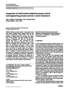
1.0 Introduction As the semiconductor industry has matured, it has become more sensitive to total operating costs. This has resulted in an increase in the amount of data collected to enhance manufacturability and product yield [1]. A frequent microlithography goal is the continuous improvement of overlay control, which can have a large impact on product yield. Automated overlay metrology systems provide an opportunity to collect extensive data sets on microlithography tools and processes. The data can be used to provide feedback in the form of correction factors to improve stepper overlay. To maximize the value of this data, it is necessary to improve and evolve monitoring and diagnostic techniques. This requires the appropriate use of statistical analysis and statistical process control (SPC) techniques. Figure 1 illustrates the typical relationship of process, stepper, metrology, analysis and SPC for a microlithography process. The wafers at the stepper are processed and a subset is sampled using in-process measurement systems for monitoring overlay and critical dimensions. Next, the measurement data is analyzed using SPC techniques with appropriate overlay models and diagnostic routines. From this analysis, essential information on the stepper and lithography processes is derived. Typical information consists of possible process alarms, optimal stepper settings of focus, exposure and overlay parameters. The output of the analysis can be used to control the stepper and processes using standard control techniques [2].
Flores, Flack, Avlakeotes and Martin
2
OCG Interface ‘95
1.1 Univariate Control Charts There are a number of different SPC and control chart techniques available to monitor individual process factors. One way to show the efficiency of the various charting techniques is to determine the average number of readings made before generating an alarm signal or control flag that a specified shift has occurred in the process mean. This metric is termed the Average Run Length (ARLz) where z is the mean shift in standard deviations. Hence, the most sensitive charting technique will have a short ARLz. In addition, it is important to minimize false alarm signals, even when the process is properly centered. A false alarm signal is specified by an ARL0 with a shift of zero standard deviations. Since data collection can be sparse in microlithography, it is typically more important to have a small ARLz than a large ARL0. The most prevalent control chart for individual factors is the Shewart chart [3]. Here, the value of a selected quality characteristic (data point) is simply plotted in time sequence and compared with standard three sigma control limits spaced above and below the process center line. A value above or below the control lines is an alarm signal or flag for corrective action. Shewart charts are popular because they are an easy charting technique to train and interpret. They were originally designed for high-volume manufacturing environments where false alarms need to be minimized. For three sigma control limits, the ARL0 of a Shewart chart is 370. However, the technique has a poor sensitivity for detecting mean shifts. The ARLz of the Shewart chart can be reduced by adding rule testing for special alarm causes. The most common special tests are the Western Electric rules [3]. However, previous studies have shown that exponentially weighted moving average (EWMA) and cumulative-sum (CUSUM) charts are superior in determining process mean shifts than the Shewart chart with Western Electric rules for stepper overlay monitoring [4]. In addition, a Shewart chart with Western Electric rules can provide more false flags than these other techniques. All of these techniques are univariate control charts and thus only monitor a single parameter or output at a time. Therefore they cannot detect changes in the relationship between multiple parameters. In conjunction with the Shewart chart for monitoring the process mean, it is useful to monitor the three sigma variability for each subgroup of measurements. The three sigma or S chart provides valuable information on the process stability. For overlay control in microlithography, a common strategy is to use Shewart mean and S charts to monitor the x and y overlay for each subgroup of wafers. While this technique is effective for overlay monitoring, it does not necessarily produce optimal overlay performance. 1.2 Overlay Control and Errors Overlay performance can be enhanced by monitoring stepper grid and lens corrections. Again, this is a major challenge due to the inherent multivariable nature of these parameters. For a microlithography system, the overlay errors can be divided into intrafield and interfield systematic sources. The intrafield sources (dX and dY) model the overlay error sources within one field [5,6]:
Flores, Flack, Avlakeotes and Martin
3
OCG Interface ‘95
dX(x,y) = Tix +Mxx - Θiy + Ψxxy + Ψyx2 + D3x(x2+y2) + D5x(x2+y2)2
(1)
dY(x,y) = Tiy + Myy + Θix + Ψyxy + Ψxy2 + D3y(x2+y2) + D5y(x2+y2)2
(2)
where x and y are the coordinate location relative to the center of the field. For equations (1) and (2), the linear terms include die shift in x (Tix) and y (Tiy), magnification in x (Mx) and y (My) and rotation (Θi). The nonlinear terms include trapezoid in x (Ψx) and y (Ψy) third order (D3) and fifth order (D5). These numerous parameters are difficult to monitor in a production environment because of the large amount of data that must be collected inside each field. Typically, these parameters are set and only periodically adjusted as part of a maintenance program [7]. The interfield or grid sources (Ex and Ey) model the stepper stage motion errors across the wafer [6]: Ex(X,Y) = Tgx + SxX - ΘxY
(3)
Ey(X,Y) = Tgy + SyY + ΘyX
(4)
where X and Y are the coordinate locations on the wafer. The interfield sources include offset error in X (Tgx) and Y (Tgy), wafer scaling magnification in X (Sx) and Y (Sy), and wafer rotation in X (Θx) and Y (Θy). These six stepper grid variables can be easily determined and monitored in production environments using in-line metrology. For optimal overlay control, it is desirable to simultaneously monitor and control these six grid parameters. One possibility is to use separate univariate control charts for each output variable. This approach has the obvious difficulty of management and analysis of a large quantity of charts. If the output variables are highly correlated, monitoring the control chart on only one output variable would be adequate. However, it is more likely for the output variables to be partially correlated to various degrees. Thus application of univariate charts for each parameter can result in misleading alarm flags due to a distortion of in-control and out-of-control events [8,9]. For a Shewart control chart with three sigma limits, the probability that the control parameter exceeds its control limits is 1/ARL0 (1/370 or 0.0027). The probability that the process is within the 3 sigma limits is simply (1 - 1/ARL0) or 0.9973. In general, for a process consisting of p statistically independent parameters being monitored, the probability that all p parameters will plot in 3 sigma control limits when they are in control is given by [9]: P{all p means plot in control}= (0.9973)p
(5)
For the case of six parameters, the probability is reduced from 0.9973 to 0.9839. The corresponding six parameter ARL0 has been reduced to 62 from 370 for a single uncorrelated univariate chart. It is important to note that equation (5) assumes that six parameters are
Flores, Flack, Avlakeotes and Martin
4
OCG Interface ‘95
statistically independent. It is more typical that the parameters are partially dependant which could produce an even smaller ARL0. 1.3 Multivariate Control Charts The original work on multivariate quality control was performed by Hotellings to enhance the accuracy of aerial bombing during World War II. The Hotellings T2 statistic provides a combined score that properly accounts for cross-correlation of multiple output variables [9]. It incorporates the components of error variance, covariance and correlation between all combinations of the output variables [10,11]. A major advantage of this multivariate control technique is in the application of real-time or direct feedback control. All six grid parameters are readily available from in-line metrology equipment. This approach contrasts with previous multivariate studies that required multiple measurements spread over time to generate a single subgroup [10]. The Hotellings T2 statistic can be used to construct a single multivariate control chart that minimizes the occurrence of false process alarms or flags as well as identifying process changes not detected using univariate charts [10,11]. Inherent to the Hotellings T2 statistic are two main components. First, it includes the parameters typical deviation from their mean values. Second, it is adjusted by the influence of the other correlated parameters deviation from their mean. The statistic takes on a low value when the cross-correlation among the six grid parameters is constant. Conversely, it takes on a larger value when there is any change with respect to one or more of the parameters. The Hotellings T2 test statistic is calculated by [9]: T2j = n [xj - xm]T S-1 [xj -xm]
(6)
where: j is the subgroup number n is the sample size for the subgroup xj is the subgroup sample mean for each parameter [vector of length p] xm is the overall sample mean for each parameter [vector of length p] S is the covariance for the parameters (matrix of size p by p) p is the number of parameters or output variables First, the covariance matrix is inverted (S-1) and multiplied by the vector corresponding to the difference between the subgroup mean and overall mean for each parameter ([xj -xm]). The resultant vector is then multiplied by the vector transpose of the same mean difference for each parameter ([xj - xm]T). Note that each subgroup (j) corresponds to an individual reading on a univariate control chart. The T2j statistic for each subgroup is then plotted on a standard control chart. For more than 25 subgroups, the upper control limit (UCL) is usually defined as χ2α,p where α is the confidence limit [9]. For a smaller number of subgroups, the UCL is based on the Fdistribution [12]:
Flores, Flack, Avlakeotes and Martin
5
OCG Interface ‘95
UCL = (knp - kp - np + p)/(kn - k - P + 1) F(α, p, kn- k - p +1)
(7)
where k is the number of subgroups in the chart. One difficulty encountered with the use of T2 control charts is the practical interpretation of an out-of-control alarm. It is difficult to determine which of the variables is responsible for the alarm. The standard practice is to plot univariate mean charts for the individual variables and look for mean excursions. In this project the overlay stability of an Ultratech stepper was monitored over a four month period. Monitor wafers were processed on the stepper and measured using a metrology tool to gauge the overlay performance. Individual control charts were generated for the modeled stepper grid parameters of x and y scale, x and y offsets and x and y rotation. The Hotellings T2 statistic was then evaluated to account for the highly correlated nature of the wafer grid parameters for stepper overlay. The average run length of the six univariate charts and multivariate control chart techniques were compared for the detection of process and tool shifts. A comparison of the univariate SPC alarm flags based on the Western Electric rules and the multivariate alarm flags demonstrates the efficiency of the Hotellings T2 statistic.
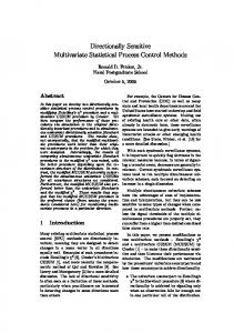
2.0 Experimental Methodology An Ultratech Stepper Model 2244i was used for the process monitoring experiments. The Ultratech stepper is based on the 1X Wynne-Dyson lens design using broadband i-line illumination from 345 to 365 nm [13]. The stepper utilizes a darkfield alignment detection system with Enhanced Global Alignment (EGA), where five fields are sampled per wafer as shown in Figure 2. The alignment targets for each EGA site are located along the horizontal scribe across the top of the stepper field. The target design is a cross with a width of 2.0 microns and a darkfield (valley) polarity. The stepper generates the six grid parameters for each wafer based on equations (3) and (4) using the five sampled EGA sites. Bare silicon wafers of 200mm diameter were used for this study. Initially, a first level mask pattern was defined in a 1.1 micron thick photoresist film. A second level was aligned and exposed in the same photoresist where the stepper applied EGA corrections to the second level. Wafers were run throughout the monitoring period without any process shift to establish a process baseline. This provided the ability to gauge the natural stepper variation during the extended fourmonth monitoring period. However, the stepper used in this study did have several engineering hardware modifications installed during the monitoring period, which potentially altered the stepper baseline. Sample wafers were processed through the stepper on a periodic basis.The photoresist-tophotoresist overlay pattern was then measured using a KLA 5700 Coherence Probe Microscope [14]. The overlay structures are a standard box-in-frame design. Characterization of the metrology
Flores, Flack, Avlakeotes and Martin
6
OCG Interface ‘95
system was performed to quantify the tool error. Multiple measurements were taken on the overlay targets during the tool setup to establish a three sigma tool variance of 7 nanometers (nm). Additionally, the Tool Induced Shift (TIS) was characterized and found to be less than 10 nm for layers up to 15 microns thick. The wafer layout consisted of 27 fields, as shown in Figure 2, with field dimensions of 44 mm in x and 22 mm in y. All the fields were sampled to reflect process variability over the entire wafer. The overlay was measured at the center of the field. A total of 4 wafers were aligned for each process subgroup run (n). Thus, each lot or process group of wafers included a total 108 measurements per subgroup run. This provides sufficient statistical degrees of freedom for extraction of the six wafer grid parameters using KLASS III® software [15]. Shewart control charts with Western Electric rules were generated for each of the six grid parameters using JMP® statistical software. The Hotellings T2 statistic was calculated using a Microsoft Excel® spreadsheet to perform the necessary matrix and vector operations.
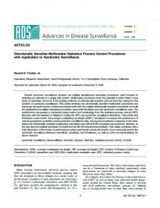
3.0 Results and Analysis 3.1 S Control Charts S control charts for both the x and y overlay offsets were calculated to establish the process dispersion or variability over the monitoring period. However, only y data will be presented since the x data displayed similar behavior. Figure 3 shows the S control chart for the y overlay component. Each value plotted for a specific run number is based on the total 3 sigma variation over the 4 wafer group described in the experimental methods section. Interpreting the behavior of the y three sigma chart provides useful insight into the process and tool stability. For run numbers 1 through 24, the overall trend shows a 3 sigma which is continuously decreasing, with an initial value of 0.110 microns to 0.040 microns. This trend is consistent with the status of the stepper during this period, where no major hardware or software modifications were implemented. Run numbers 24 through 28 show a larger three sigma variability. The assignable cause for this excursion was an experimental hardware modification on the stepper wafer stage. This hardware was installed for system testing purposes. During runs 24 to 28 slight modifications of the stepper were implemented to characterize the hardware modification. At run number 29, the stepper was returned to its previous configuration. Similar behavior was also observed with x three sigma variability. While the S control chart is useful for monitoring overlay stability, it does not provide information to enhance stepper overlay performance. This requires the evaluation of control charts for the stepper grid parameters.
Flores, Flack, Avlakeotes and Martin
7
OCG Interface ‘95
3.2 Univariate Control Charts The six univariate control charts for the individual grid parameters are shown in Figures 4 through 9. Each value plotted at a specific run number is determined by a regression analysis of equations (3) and (4) for that subgroup of 4 wafers using KLASS III® software. The control charts are Shewart type and include Western Electric Rules. The rules are highlighted on the charts by the numbers 1 through 6. The rules are numbered in descending order of the seriousness of the rule violation. Figures 4 and 5 display the x and y grid offset control charts in microns along with the three sigma control limits and Western Electric Rules. Of the 42 runs, there are 11 runs with alarm flags for the x offset and 5 runs with alarms for the y offset. The x offset control chart shows several apparent alarms during the first 24 runs which have no apparent or assignable cause. Runs 8 and 9 are flagged with a type 1 alarm since they are outside the upper three sigma control limits. In addition, a type 1 alarm is detected at run 25, which corresponds to the hardware modification previously discussed. The runs following 25 also suggest an excursion of the stepper and thus support the known stepper baseline disturbance. Overall, the high frequency of alarm signals on the x offset chart makes determination of the ARL a difficult task. The y grid offset is less severe in terms of flagged alarms. A type 6 alarm is flagged at run 28, which is based on 4 out of 5 points in a row being at least 2 standard deviations above the average value. This usually indicates a shift in the process mean and is also consistent with the system hardware modification. However, the remaining four Western Electric alarms have no assignable cause. Figures 6 and 7 display the x and y grid scale control charts in parts per million (ppm) along with the three sigma control limits and Western Electric Rules. Of the 42 runs, there are 28 runs with alarm flags for the x grid scale and seven runs with alarms for the y grid scale. It is readily apparent that a shift in mean value of the x scale occurs after run number 14. This mean shift results in a bimodal distribution and produces many false alarm flags since a normal distribution is assumed for a Shewart control chart. Hence, extensive flagging of runs should not be assumed to be valid. The source of this shift in the x scale was a change in the settings of the stepper wafer stage. Again like the x grid offset, the high frequency of alarm signals makes determination of the ARL a difficult task for this control chart. A more subtle mean shift appears on the y scale after run number 14. However, there are no Western Electric flags indicating this shift. This is probably due to the larger spread in the individual runs proceeding run number 14. The final two runs 41 and 42 are both flagged with a type 1 alarm since they are outside the upper 3 sigma control limit. The last two univariate control charts are the x and y rotation in microradians with the three sigma control limits as shown in figures 8 and 9. Unlike the previous four control charts, these parameters are generally well behaved with only a single type 1 alarm at run 34 on x rotation.
Flores, Flack, Avlakeotes and Martin
8
OCG Interface ‘95
3.3 Output Variable Correlation The univariate control charts in the previous section assume that the six grid parameters are statistically independent. Table 1 shows the partial correlation matrix over the 42 run baseline. Each value in the table represents the partial correlation between various pairs of grid parameters. The corresponding labels in the row and column identify the appropriate pair for each entry. The main diagonal of the matrix shows a value of 1.0000 since each grid parameter is directly correlated to itself. A measure of the relationship or coupling between each pair of grid values is indicated by the size of the partial correlation values, where a 1 indicates a direct coupling and a 0 indicates no dependence of the variables. Since every value in the table is nonzero, there is a partial correlation among the entire set of grid values. This validates the necessity of using a T2 statistic rather than individual control charts. Of particular significance is the large correlation value of 0.5580 for the x and y rotation. This means that 55.8% of the variability of x rotation accounts for the variability of y rotation. 3.4 Multivariate Control Chart The calculation of the Hotellings T2 statistic requires an estimate of the mean values for all the six grid parameters and their corresponding partial covariance matrix. Once these values are calculated, they can be used in equation (6) to determine a T2 value for each individual run. Note that the Hotellings T2 statistic takes on a low value when the cross-correlation among the six grid parameters is constant. Conversely, it takes on a larger value when there is any small change with respect to one or more of the parameters. Figure 10 displays the Hotellings T2 control chart based on the six stepper grid parameters. This chart is constructed with a single upper control limit based on the χ2α,p. A confidence limit of 0.005 (α) for 6 factors (p) was used for the calculation of χ2α,p. Any T2 value exceeding this upper control limit of 22.0 generates an alarm signal or flag that the relative correlation of the individual parameters has changed or the process mean vector has shifted. Only run numbers 9, 25, 33, 34 and 42 are flagged since they exceed the upper control limit. Run 25 corresponds to the engineering hardware modification to the system. The remaining runs 9, 33, 34 and 42 do not have a direct assignable cause and indicate an additional source of variation that is not being monitored. Thus the Hotellings T2 control chart shows the ability to flag process shifts as well as other unmonitored variations within the system. 3.5 SPC Error Flags Comparison For monitoring and control of this stepper process, it is helpful to compare three separate techniques for determining alarm conditions. The first is to count the total number of alarm flags generated by application of the Western Electric Rules for the six univariate control charts. A second more conservative technique is to count the Shewart three sigma control alarms generated for each of the six univariate control charts. The final technique is to use the single multivariate
Flores, Flack, Avlakeotes and Martin
9
OCG Interface ‘95
control chart approach based on Hotellings T2 statistic with an upper control limit. Figure 11 compares the number of alarms or flags generated based on the three schemes for each run number or process subgroup. Of the three schemes, the Western Electric Rules generate the highest incidence of false alarm signals and do not provide a clear indication of the known or assignable process shifts. This corresponds to the observed problem of false alarms using univariate control charts to monitor multiple outputs when there is cross-correlation of the outputs. The Shewart three sigma flags are less abundant than the Western Electric rules and do flag run number 25 which corresponds to the system hardware modification. However, there are still several apparent alarms during the first 10 runs. Alarm flags based on Hotellings T2 statistic show the least occurrence of false signals. It is also interesting that all the Shewart alarms are included in the Hotellings T2 chart. This illustrates the efficiency of a single multivariate chart for monitoring the entire set of grid parameters.
4.0 Conclusions In this project, the overlay stability of a stepper was monitored over a four-month period using conventional univariate control charts and a single multivariate control chart. The six modeled stepper grid parameters of x and y scale, x and y offsets and x and y rotation were monitored during this period. Based on these six univariate control charts, a high frequency of alarm signals was generated using the Western Electric Rules. Consequently, the ability to clearly identify process shifts of the stepper was ambiguous. Close examination of the six grid parameters showed several cross-correlations. For example, there was a large correlation of the x and y grid rotation terms. These results support the known problems that occur when using multiple control charts for correlated outputs. Based on the multivariate Hotellings T2 statistic control chart, the frequency of false alarm signals was reduced. The technique also demonstrated the ability to detect process shifts. This single multivariate chart is also simpler to manage and interpret as compared to the six individual univariate charts. A major advantage of this multivariate control technique is the application of real-time or direct feedback control since all six grid parameters are readily available from in-line metrology equipment. The implementation and effective use of multivariate techniques in lithography manufacturing requires automated software to support generation of the Hotellings T2 statistic control chart. At present, there is a lack of readily available software for implementing this technique. In the future the microlithography industry will need more sophisticated software to support multivariate techniques.
Flores, Flack, Avlakeotes and Martin
10
OCG Interface ‘95
5.0 References 1. D. Miller, F. Anatasio, “World Class Manufacturing: CIM or Sink” IEEE/SEMI International Semiconductor Manufacturing Science Symposium, (1991). 2. G. Flores, W. Flack, J. Pellegrini, M. Merrill, “Registration Simulation for Large Field Lithography”, OCG Microlithography Seminar, Interface ‘94 Proceedings, (1994). 3. Statistical Quality Control Handbook, Western Electric Company (1956). 4. G. Flores, W. Flack, S. Avlakeotes, M. Merrill, “Monitoring and Diagnostic Techniques for Control of Overlay in Steppers”, SPIE Integrated Circuit Metrology, Inspection and Process Control IX Proceedings, SPIE 2439 (1995). 5. J. Armitage, “Analysis of Overlay Distortion Patterns”, Integrated Circuit Metrology, Inspection and Process Control II Proceedings, SPIE 921 (1988). 6. M. van den Brink, C. de Mol and R. George, “Matching Performance for Multiple Wafer Steppers Using an Advanced Metrology Procedure”, Integrated Circuit Metrology, Inspection and Process Control II Proceedings, SPIE 921 (1988). 7. A. Yost, W. Wu, “Lens Matching and Distortion in a Multi-Stepper, Submicron Environment”, Integrated Circuit Metrology, Inspection and Process Control III Proceedings, SPIE 1087 (1989). 8. H. Guo, C. Spanos, A. Miller, “Real Time Statistical Process Control for Plasma Etching”, IEEE/SEMI International Semiconductor Manufacturing Science Symposium Proceedings, (1991). 9. D. Montgomery, Introduction to Statistical Quality Control, New York: John Wiley & Sons (1985). 10. W. Levinson, “Statistical Process Control in Microelectronics Manufacturing”, Semiconductor International, November 1994. 11. C. Smith, W. Roberts, T. Bell, “An Advanced Critical Dimension and Monitoring Method, Using Multivariate Control Charts”, OCG Microlithography Seminar Interface ‘94 Proceedings, (1994). 12. T. Ryan, Statistical Methods for Quality Improvement, New York: John Wiley & Sons (1989). 13. R. Hershel, “Characterization of the Ultratech Wafer Stepper”, Optical Microlithography Proceedings, SPIE 334 (1982). 14. M. Davidson et. al., “First Results of a Product Utilizing Coherence Probe Imaging for Wafer Inspection”, Integrated Circuit Metrology, Inspection and Process Control II Proceedings, SPIE 921 (1988). 15. KLASS III® Reference Manual, Appendix Models and Algorithms.
Flores, Flack, Avlakeotes and Martin
11
OCG Interface ‘95
Stepper
Measurement Station
˚ 5015
Analysis Station
Process Alarms Stepper Settings Focus, Exposure Grid, Intrafield
SPC Analysis Stepper Models Diagnostic Models
Figure 1: Relationship of process, stepper, metrology, analysis and statistical process control.
EGA Sample Site
Figure 2: Wafer layout and EGA scheme for alignment monitoring.
Flores, Flack, Avlakeotes and Martin
12
OCG Interface ‘95
0.3
Y Three Sigma
0.25 0.2 0.15
■
■
■
0.1
■
0.05
■
■
■ ■
■
■
■
■ ■
■
■
■
■ ■ ■
■
■■■
■ ■
■
■
■■
■ ■
■ ■
■ ■
■■■ ■
■
■■
0 0
5
10
15
20 25 30 Run Number
35
40
45
Figure 3: S control chart for y alignment error containing 42 subgroups of four wafers each monitored over a period of four months.
X Offset
Y Offset
X Scale
Y Scale
X Rot
Y Rot
X Offset
1.0000
0.1723
0.3008
-0.2263
0.2877
0.2686
Y Offset
0.1723
1.0000
-0.2923
-0.0320
-0.1442
-0.1831
X Scale
0.3008
-0.2923
1.0000
-0.1903
-0.1164
0.0824
Y Scale
-0.2263
-0.0320
-0.1903
1.0000
-0.2410
-0.2828
X Rotation
0.2877
-0.1442
-0.1164
-0.2410
1.0000
0.5580
Y Rotation
0.2686
-0.1831
0.0824
-0.2828
0.5580
1.0000
Table 1: Partial correlation matrix for the six stepper grid parameters.
Flores, Flack, Avlakeotes and Martin
13
OCG Interface ‘95
0.1
11 ■
1
■
■
UCL = 0.069
■ ■
X Offset (microns)
0.05
■
2 ■
■
■
5■
■ ■
0
■
■
■
■■
■
6
■
■
■
■
■
■
■
■
■■
3
6
■■
-0.05
■ ■
■
3
AVG = -0.002
■ ■■
■
■
■■
2
5
■
■
LCL = -0.065 -0.1 0
5
10
15
20 25 30 Run Number
35
40
45
Figure 4: Control chart with Western Electric rules for the x offset grid model parameter. The alarm signals are numbered as to seriousness.
0.1 0.08
Y Offset (microns)
0.06
■
0.04
■
■■
■■
■
■
0.02
■ ■
■
-0.02
■ ■
■ ■
■
2
■
■
■
■ ■
■ ■
-0.04
■
-0.06
■
■
■ ■
■■
■
■
5
0
UCL = 0.0585
6
■
■■■
■
■
5
AVG = -0.0055 ■
■
■
LCL = -0.0695
■
-0.08
1
-0.1 0
5
10
15
20 25 30 Run Number
35
40
45
Figure 5: Control chart with Western Electric rules for the y offset grid model parameter.
Flores, Flack, Avlakeotes and Martin
14
OCG Interface ‘95
0.7
1
0.5
■1
■■
1
■
0.3 X Scale (ppm)
■
11
■
1
■■
5 5 0.1
UCL = 0.29
■2
2
2■■■■ 22
■
6
-0.1
■ ■■
■
-0.3
6
■
-0.5
■ ■ ■2
■
■
■
■
2
■■
■
2 ■■■
■
6
■
■
■
■22
AVG = -0.11
5
■2
■
■
■ 5 53
■6
6 LCL = -0.52
-0.7 0
5
10
15
20 25 30 Run Number
35
40
45
Figure 6: Control chart with Western Electric rules for the x scale grid model parameter.
0.5
1 1■ ■
0.3
■
Y Scale (ppm)
■ ■ ■■
■
■
■■■
■
■
-0.1
■
■
■
■5 ■
■
■ ■
■
AVG = 0.04
■■ ■
■ ■
■
5
-0.3
■
■
■
2
■■
■■
6■ ■
■
■
■
0.1
UCL = 0.37
■
LCL = -0.30
5
-0.5 0
5
10
15
20 25 30 Run Number
35
40
45
Figure 7: Control chart with Western Electric rules for the y scale grid model parameter.
Flores, Flack, Avlakeotes and Martin
15
OCG Interface ‘95
1.4 ■1
X Rotation (microradian)
1.2
UCL = 1.13
1 0.8 0.6
■
■
■
■
■
0.4 ■
0.2
■
■■
■
■
0 -0.2
■
■■
■■
AVG = 0.09
■
■ ■
■
■
■
■
■■
■■ ■
-0.4 -0.6
■
■
■ ■
■
■■
■
■
■ ■
■
-0.8 -1
■
0
5
10
15
20 25 30 Run Number
35
LCL = -0.94
40
45
Figure 8: Control chart with Western Electric rules for the x rotation grid model parameter.
0.8 UCL = 0.65
Y Rotation (microradians)
0.6 ■
0.4 ■
■
0.2
■
■■
0 -0.2
■
■
■■
■
■
■
■
■ ■
■
■
■
■
■ ■
■ ■
■
■ ■
■
■
■
■■
■■
AVG = -0.13
■
■
-0.4
■
■
■
-0.6
■
-0.8
■
■
LCL = -0.91
-1 0
5
10
15
20 25 30 Run Number
35
40
45
Figure 9: Control chart with Western Electric rules for the y rotation grid model parameter.
Flores, Flack, Avlakeotes and Martin
16
OCG Interface ‘95
45 ■
40
■
Hotellings T2 Value
35 30
■
■
25
■
UCL = 22.0
20
■ ■■
15
■ ■
■
10
■
■
■■■
■ ■
■
■
■■ ■ ■
5
■ ■
■
■
■
■
■
■ ■■■
■■
■■
■
■
■
0 0
5
10
15
20 25 30 Run Number
35
40
45
Figure 10: Control chart of the Hotellings T2 statistic.
4
Western Electric Flags
3
Number of Flags
2 1 0
Shewart 3 Sigma Flags
3 2 1 0
Hotellings T2 Flags
1 0 0
5
10
15
20 25 30 Run Number
35
40
45
Figure 11: Comparison of the alarm signal flags generated for the Hotellings T2 statistic, Shewart three sigma charts and control charts with Western Electric rules for each subgroup.
Flores, Flack, Avlakeotes and Martin
17