"Process Systems Engineering, 9. Domain Engineering," in ...

Process Systems Engineering, 9. Domain Engineering IOANNIS G. ECONOMOU, The Petroleum Institute, Department of Chemical Engineering, Abu Dhabi, United Arab Emirates EFSTRATIOS N. PISTIKOPOULOS, Imperial College London, Department of Chemical Engineering, London, United Kingdom JEN-PEI LIU, Imperial College London, Department of Chemical Engineering, London, United Kingdom YOSHIAKI KAWAJIRI, Georgia Institute of Technology, School of Chemical & Biomolecular Engineering, Georgia I, Atlanta, United States KRIST V. GERNAEY, Center for Process Engineering and Technology, Department of Chemical and Biochemical Engineering, Technical University of Denmark, Lyngby, Denmark JOHN M. WOODLEY, Center for Process Engineering and Technology, Department of Chemical and Biochemical Engineering, Technical University of Denmark, Lyngby, Denmark CONCEPCIOŃ JIMEŃEZ-GONZA´LEZ, GlaxoSmithKline, Research Triangle ParkNorth Carolina, United States RENE´ BANÃRES-ALCAŃTARA, University of Oxford, Department of Engineering Science, Oxford, United Kingdom

1.

1.1. 1.2. 1.3. 1.3.1. 1.3.2. 1.4. 1.4.1. 1.4.2. 1.4.3. 1.5. 2. 2.1. 2.2. 2.2.1. 2.2.2. 2.2.3. 2.2.4. 2.2.5. 2.3. 2.3.1.

Molecular Modeling and Simulation for Chemical Product and Process Design . . . . . . . . . . . . . . . . . . . . . . . . . 2 Introduction. . . . . . . . . . . . . . . . . . . 2 Elementary Statistical Mechanics . . 3 Major Molecular Simulation Methods 3 Molecular Dynamics (MD) . . . . . . . . 3 Metropolis Monte Carlo Simulation . . 4 Applications . . . . . . . . . . . . . . . . . . . 4 Pharmaceuticals. . . . . . . . . . . . . . . . . 4 Polymer Membranes for Gas Separation 6 Ionic Liquids for Sustainable Chemical Processes . . . . . . . . . . . . . . . . . . . . . 8 Conclusions . . . . . . . . . . . . . . . . . . . 9 Energy Systems Engineering . . . . . . . 10 Introduction. . . . . . . . . . . . . . . . . . . 10 Methods/Tools/Algorithm . . . . . . . . 10 Superstructure-Based Modeling . . . . . 10 Mixed-Integer Programming (MIP) . . . 11 Multiobjective Optimization. . . . . . . . 11 Optimization under Uncertainty . . . . . 11 Life-Cycle Assessment . . . . . . . . . . . 12 Energy Systems Examples . . . . . . . . 12 Example 1–Polygeneration Energy Systems . . . . . . . . . . . . . . . . . . . . . . 12

2012 Wiley-VCH Verlag GmbH & Co. KGaA, Weinheim 10.1002/14356007.o22_o13

2.3.2. Example 2–Hydrogen Infrastructure Planning . . . . . . . . . . . . . . . . . . . . . . 2.3.3. Example 3–Energy Systems in Commercial Buildings . . . . . . . . . . . . 2.4. Conclusions and Future Directions . 3. Pharmaceutical Processes . . . . . . . . . 3.1. Introduction. . . . . . . . . . . . . . . . . . . 3.2. Pharmaceutical Process Development and Operation . . . . . . . . . . . . . . . . . 3.2.1. Crystallization . . . . . . . . . . . . . . . . . . 3.2.2. Chromatography . . . . . . . . . . . . . . . . 3.3. Conclusion . . . . . . . . . . . . . . . . . . . . 4. Biochemical Engineering . . . . . . . . . . 4.1. Introduction. . . . . . . . . . . . . . . . . . . 4.2. Industrial Biotechnology Processes . 4.2.1. Fermentation Processes . . . . . . . . . . . 4.2.2. Microbial Catalysis . . . . . . . . . . . . . . 4.2.3. Enzyme Processes . . . . . . . . . . . . . . . 4.3. Modeling of Bioprocesses. . . . . . . . . 4.3.1. Modeling of Bioprocesses– Mechanistic Models. . . . . . . . . . . . . . 4.3.2. Modeling of Bioprocesses–DataDriven Models . . . . . . . . . . . . . . . . . 4.4. The Role of Process Systems Engineering . . . . . . . . . . . . . . . . . . .

15 17 18 19 19 20 21 22 25 25 25 26 26 27 27 28 28 29 30

2

Process Systems Engineering, 9. Domain Engineering

4.4.1. 4.4.2. 4.4.3. 4.4.4. 4.4.5. 4.5. 4.5.1. 4.6. 5. 5.1. 5.2. 5.3. 5.4. 5.5. 5.6. 5.7. 5.7.1. 5.7.2. 5.7.3.

Evaluation of Process Options . . . . . . Evaluation of Platform Chemicals . . . Process Integration . . . . . . . . . . . . . . Biorefinery Design. . . . . . . . . . . . . . . Biocatalyst Design. . . . . . . . . . . . . . . Assessing the Sustainability of Bioprocesses. . . . . . . . . . . . . . . . . Life-Cycle Inventory and Assessment. Future Outlook and Perspectives. . . Policies and Policy Making . . . . . . . . Introduction. . . . . . . . . . . . . . . . . . . Policies and Policy Measures . . . . . . Policy Making and the Systems Approach . . . . . . . . . . . . . . . . . . . . . Similarities between Policy Formulation and Conceptual Process Design . . . . The Nature of Policy Formulation . . The Nature of Sociotechnical Systems Challenges for Modelers of Sociotechnical Systems. . . . . . . . . . . Multiple Stakeholders . . . . . . . . . . . . Incommensurable Values . . . . . . . . . . Externalities . . . . . . . . . . . . . . . . . . .

30 30 31 31 31

5.7.4. 5.7.5. 5.7.6. 5.7.7. 5.8.

32 33 35 36 36 36

5.8.1.

36 37 38 39 39 39 39 40

1. Molecular Modeling and Simulation for Chemical Product and Process Design 1.1. Introduction Major chemical process industries (CPI) have experienced a substantial transformation in recent years worldwide due to an increased competition at a global level and a significant pressure from national governments and international organizations to develop new sustainable processes that consume significantly smaller quantities of energy and other natural resources and operate under zero (or close to zero) waste production. In parallel, major multinational CPI shifted from low value commodity products to specialty products of high added value where the underlined materials are of considerably higher complexity in terms of: . . . .

Chemical structure Molecular and supramolecular architecture Micro- and mesostructure Performance in the end-use environment

5.8.2. 5.8.3. 5.8.4. 5.8.5. 5.8.6. 5.8.7. 5.8.8. 5.8.9. 5.9. 5.10.

Uncertainty . . . . . . . . . . . . . . . . . . . . Emergent Behavior . . . . . . . . . . . . . . Complexity of Causation . . . . . . . . . . Objectivity in Policy Analysis . . . . . . Types of Models Used in the Analysis of Policies. . . . . . . . . . . . . . . . . . . . . . . Macroeconomic Models (Mainstream, Descriptive, Aggregated, Mechanistic) Optimization Models (Mainstream, Normative, Aggregated, Mechanistic). Control Models (Mainstream, Normative, Aggregated, Mechanistic) . . . . . . . . . Data-Based Models . . . . . . . . . . . . . . Game Theory (Descriptive) . . . . . . . . System Dynamics (Aggregated, Mechanistic) . . . . . . . . . . . . . . . . . . . Network Theory (Descriptive) . . . . . . Agent-Based Approaches . . . . . . . . . . Some Conclusions on Models for the Analysis of Policies . . . . . . . . . . . . . . Synthesis of Policies . . . . . . . . . . . . . Future Directions . . . . . . . . . . . . . .

40 40 40 40 41 41 42 42 42 42 42 42 43 43 43 44

These are nontrivial changes that require concerted effort at different levels: basic research to develop fundamental knowledge of physical phenomena, applied research to develop physical models and parameters, and development work for the generation of new processes that meet the requirements stated above. Accurate simulation and optimization methodologies are necessary at all length and time scales, from the submolecular level all the way to the macroscopic level where thermodynamic and computational fluid mechanics models together with advanced numerical methods are used in a concerted way. A consistent hierarchical development of physical models is of outmost importance. This chapter refers to the development of molecular modeling and simulation methods for the design of new chemical products and the improvement of existing and design of new processes. Molecular simulation was introduced in the 1950s [1, 2] (! Molecular Modeling, Chapter 3) as an abstract physical application for the primitive computers of the time and it evolved to a powerful engineering tool more than 50 years later. At the same time, the need for further development of simulation methods


and physically accurate models remains as it will be seen later in this chapter.

1.2. Elementary Statistical Mechanics

3

along the way in order that Equation (3) can lead to meaningful results [4]. Alternatively, one may calculate a macroscopic property P as a statistical average over all microstates of the system, that is: Z

In statistical mechanics (! Molecular Dynamics (MD) Simulation), the properties of a bulk chemical system are calculated based on the collective interactions between the molecules that make up the system. Almost all of the systems of interest to process systems engineering (PSE) follow Boltzmann statistics and so the partition function (Q) of a system of constant number of molecules (N) in a specific volume (V) and temperature (T) is [3]: Z

Q¼c

dpN drN exp½HðrN pN Þ/kB T

ð1Þ

where rN and pN denote the coordinates and momenta of all N molecules, HðrN pN Þ is the Hamiltonian of the system and c is a proportionality constant. For a system of N identical (indistinguishable) molecules: c ¼ 1/ðh3N N!Þ where h is the Planck’s constant. The Hamiltonian provides the total energy of the system as a function of the coordinates and the momenta of the molecules and is given as the sum of the kinetic energy (K) and the potential energy (U), so that: HðrN pN Þ ¼

X

p2i /ð2mi ÞþUðrN Þ

ð2Þ

dpN drN PðrN pN Þexp½HðrN pN Þ/kB T Z dpN drN exp½HðrN pN Þ/kB T

hPi ¼

ð4Þ

Even then, calculation of hPi using brute force numerical integration requires extraordinary computing power. For example, for a 100 molecule system using Simpson’s rule with just 5 equidistant points along each coordinate axis one needs to evaluate the integrand of Equation (4) at 10210 points [5]. A much more efficient approach is based on the observation that some configurations of the molecular system are much more important than others, so one should focus on sampling these important configurations rather than random configurations. This has been the basis of the so-called Metropolis Monte Carlo simulation method discussed briefly below.

1.3. Major Molecular Simulation Methods 1.3.1. Molecular Dynamics (MD)

i

The potential energy U depends strongly on the nature (complexity) of molecular interactions [3]. Intermolecular potentials range from primitive potentials (such as hard sphere, square well, etc.) to potentials of moderate complexity (such as Lennard–Jones, Stockmayer, etc.) and all the way to complex potentials that account for intra- and intermolecular interactions, many body effects (polarizable potentials), etc. From the partition function, one may calculate macroscopic thermodynamic properties using the so-called bridge function, which for the case of the constant NVT system (canonical statistical ensemble) is [3]: AðNVTÞ ¼ kB T ln QðNVTÞ

ð3Þ

where A is the Helmholtz free energy. Unfortunately, the partition function Q can be calculated analytically only for a very few simple systems and significant approximations are needed

In classical (Newtonian) mechanics, the following set of equations describes the evolution of the system over time [6]: mi r€i

¼

fi

fi

¼

rri UðrN Þ

i ¼ l; . . . ; N

ð5Þ

where mi is the mass of molecule i and fi is the force exerted on it. MD consists of solving these N second order differential equations numerically using a number of different methods developed for this purpose. In this way, MD allows monitoring of the evolution of the system with time, and thus, time-dependent structure (polymer chain relaxation, etc.) and physical properties (such as viscosity, diffusion coefficient, etc.) can be calculated. MD is usually performed in the microcanonical (NVE) statistical ensemble; however, the method has been extended to canonical (NVT), isobaric-isothermal (NPT) and other statistical ensembles [6]. An important parameter concerning the robustness of the

4


MD simulation is the time step used for the numerical integration of the equations of motion. For systems characterized by a relatively stiff potential (e.g., the case of chain molecules), a typical time step is in the order of 0.1–1 fs. A number of advanced simulation techniques allow the use of different time steps for different types of forces. For example, a short time step is used for fast varying forces, such as bond stretching and bond angle bending and a longer time step is used for slowing varying forces, such as nonbonded intra- and intermolecular interactions. Using state of the art computing facilities, one may simulate a real system today (April 2010) for up to a few micro seconds. This is sufficient for the calculation of properties such as chemical potential and self-diffusion coefficient in systems that consist of small- and medium-size molecules. For the calculation of dynamic properties of long chain molecules (e.g., polymers with a molecular mass higher than 10000), alternative methods are needed [7]. 1.3.2. Metropolis Monte Carlo Simulation Metropolis Monte Carlo (MMC) simulation is a stochastic method that allows efficient sampling of the multidimensional phase space of the system. In other words, this method allows ‘‘jumps’’ in the phase space and so, no real time monitoring of the system is possible. In MMC, the different states of the system are visited with a probability proportional to the Boltzmann factor of the energy of the system [5]. The system goes from one configuration (state) to the next configuration (state) based on different types of moves that satisfy microscopic reversibility and preserve the macroscopic properties of the system that are set constant. In this way, MC simulations are performed in the NVT, grand canonical (mVT), NPT and many other statistical ensembles, depending on the system (pure fluid or mixture) and conditions (one phase, two, or more phases, etc.) examined. In a typical NVT MMC simulation, particles are displaced randomly one at a time within the simulation box and the new configuration is accepted or rejected according to the Boltzmann factor of the energy difference between the two states, that is: pNVT ¼ min½1; expðDU/ðkB TÞÞ

ð6Þ

where DU ¼ U(new) U(old) is the energy difference between the old and the new configuration. Thermodynamic properties are calculated based on Equation (4). Additional moves in the NPT, mVT and other ensembles include volume fluctuation, random insertion and deletion of particles and so on, and acceptance criteria are modified accordingly. A major breakthrough in molecular simulation was the development of the Gibbs ensemble MC (GEMC) method which allows the simultaneous simulation of several phases in equilibrium (e.g., vapor–liquid equilibrium) [8]. The method has been successfully applied to pure components, binary and multicomponent mixtures, and different types of phase equilibria (vapor–liquid, liquid–liquid, vapor–liquid–liquid, etc.) [9]. Development of efficient elementary moves for long chain molecules has also been a very active area of research over the last two decades. A broad range of moves has been proposed for the efficient relaxation of chain tails, internal segments, branch points, and even moves that allow exchange of molecular segments between two different chain molecules [10]. A combination of these moves allows today accurate simulation of polymer melts with a molecular mass of the order of several thousand.

1.4. Applications 1.4.1. Pharmaceuticals Hydration energy plays a significant role in biological processes and is currently an important predictive index for molecule availability in the pharmaceutical industry. During the complex process of driving a molecule from an aqueous phase to a target protein active site, the driving force is directly related to the difference between the hydration energy of the drug and the drug–protein association energy. Moreover, desolvation of both protein site and drug molecule occurs during this binding process, and recently developed docking/scoring methods estimate this desolvation correction based on free energy calculations. For some drug molecules, solvation free energies may be estimated experimentally from concentration measurements in two-phase systems. However, in most cases this is not possible and so accurate theoretical or computational approaches are


needed. Molecular simulation using realistic potential models is able to provide accurate estimate of the property of interest and at the same time a quantitative insight regarding the molecular mechanisms associated with the hydration. Recently, a simple thermodynamic cycle was proposed to calculate the hydration Gibbs free energy, DhydG (P,T), of complex solute molecules [11]: Solute ðwaterÞ Dhyd G" Solute ðvacuumÞ

Dwater G ! Dvacuum G !

Dummy ðwaterÞ #Ddummy G Dummy ðvacuumÞ

where, Dwater G is the Gibbs energy associated with the mutation of the solute molecules into molecules of dummy atoms (atoms that do not interact with their environment) in water, Dvacuum G is the Gibbs energy associated with the same process in vacuum, and finally Ddummy G can be seen as the hypothetical hydration Gibbs energy of dummy species. In practice, these atoms have no intermolecular electrostatic or van der Waals interactions, but their intramolecular bonded interactions are the same as in the solute atoms. As a consequence, Ddummy G is equal to zero and one can write the following equation for the thermodynamic cycle:

Dhyd G ¼ Dvacuum GDwater GDdummy G ¼ Dvacuum GDwater G

5 ð7Þ

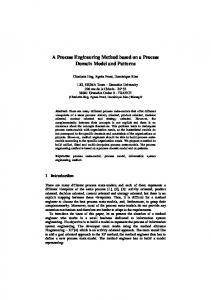
The term Dvacuum G contains only contributions from intramolecular nonbonded interactions (forces acting between atoms in the same molecule separated by more than three bonds), which exist in the solute molecule but not in the dummy molecule. The thermodynamic integration approach was used by [11] to calculate DhydG of barbituric acid and various substituted barbiturates at 298 K and 0.1 MPa. In Figure 1, DhydG and the Lennard–Jones contribution to it, DLJG, are presented as a function of molecular mass for various mono- and di-substituted barbiturates. Using the same methodology, DhydG of various n-alkanes [12] and polar compounds [13] were calculated by [11]. An extensive evaluation of three widely used molecular models (force fields) to describe the polar compounds, namely TraPPE, Gromos and OPLS-AA, was performed. In all cases, the MSCP/E model was used for water. An overview of the predictions obtained from the different force fields for the polar compounds and a comparison with experimental data is shown in Figure 2. For the relatively simple polar molecules, such as methanol and propanol, all force field predictions are in good agreement with experimental data. For the case of more complex multifunctional molecules, including acetylsalicylic acid (ASA) and ibuprofen (IBP) that are of interest to phar-

Figure 1. MD predictions of DhydG and of DLJG against molecular mass for various mono- and di-substituted barbiturates at 298 K BA ¼ barbituric acid, MB ¼ methyl barbiturate, EB ¼ ethyl barbiturate, iPB ¼ isopropyl barbiturate, BAR ¼ barbital, PRO ¼ probarbital, BUT ¼ butethal, PEN ¼ pentobarbital

6


Figure 2. Experimental data and MD predictions of DhydG of various polar molecules using different force fields at 298 K a) Methanol; b) Propanol; c) Ethylamine; d) Acetone; e) Acetic acid; f) IBP; g) ASA; h) Benzoic acid

maceutical industry, MD predictions from different force fields deviate and the agreement with experiments is less satisfactory. 1.4.2. Polymer Membranes for Gas Separation Polymeric membranes (either glassy or elastomeric) are used widely for separation of mixtures in chemical industry, medical applications, etc. A major physical property in such a process is the permeability (P) of component i in the polymer membrane defined as the product of the solubility (S) and diffusivity (D), so that: P ¼ SD

ð8Þ

Separation of a binary mixture of components i and j (where i is typically the most permeable of the two components) by a given polymer membrane is characterized by the ideal separation factor, which is the ratio of permeabilities for components i and j according to the expression: aid ij ¼

Pi ¼ Pj

Si Di Sj Dj

ð9Þ

where the ratios aSij ¼ Si /Sj and aD ij ¼ Di /Dj represent the solubility selectivity and the diffusivity selectivity, respectively. In rubbery S polymers aD ij is less than unity, while aij 1, so ideal separation factor is governed by selectivity of sorption. Polydimethylsiloxane (PDMS) is a widely used polymer membrane

and so ideal separation factors for various binary gas and liquid mixtures have been measured. The separation factor for n-C4H10/CH4 mixture is used widely as a benchmark for hydrocarbon mixture separation capability of a given membrane material. A new atomistic force field was developed for PDMS that accounts for bond stretching, bond angle bending, dihedral angle torsion, and nonbonded intra- and intermolecular interactions [14]. For the nonbonded interactions, the Lennard–Jones potential for shortrange van der Waals repulsive and attractive interactions together with a long-range Coulombic potential were used. The model was shown to predict accurately the thermodynamic properties of polymer melts over a wide temperature and pressure range [14]. It was further used for polymer–gas mixture simulations. In Figure 3, pure gas n-C4H10/CH4 solubility, diffusivity, and permeability selectivities in the range of 273–400 K calculated from MD simulations together with experimental data from [15] are shown. The solubility of hydrocarbons in the polymer matrix was based on the Widom’s test particle insertion method that allows accurate calculation of the excess chemical potential of the solute in the solvent. MD simulation of the polymer matrix for 5–10 ns followed by several hundred thousands of solute molecule insertions in each polymer configuration (this is a relatively fast post-processing calculation) provides an accurate estimate of the solubility.


7

Figure 3. n-C4H10–CH4 mixture behavior in PDMS as a function of temperature A) Solubility (S) selectivity; B) Diffusivity (D) selectivity; C) Permeability (P) selectivity Open symbols are experimental data [15] and closed symbols are MD predictions

For the calculation of diffusion coefficient, significant longer MD simulations, on the order of 100 ns, are needed in order to ensure that the hydrocarbon molecules diffusing through the polymer matrix reach the normal diffusing (Fickian) regime [16]. In this case, the diffusion coefficient is calculated from the mean square displacement of the hydrocarbon molecules, based on Einstein equation. Figure 3 reveals that solubility selectivity decreases significantly as temperature increases while diffusivity selectivity increases but with a smaller rate. Finally, the ideal separation factor follows closely the trend exhibited by solubility selectivity. In all cases, MD predictions are in excellent agreement with experiments [15] over the entire temperature range. For the accurate design of a polymer membrane for the separation of a real mixture, mixture permeability data are needed. It is often assumed that in rubbery polymers penetrants permeate independently of one another. However, this behavior needs to be confirmed for a given system. Recent experimental data for the

n-C4H10–CH4 mixture in PDMS showed an increase in CH4 solubility in the presence of n-C4H10 in the polymer. On the other hand, only a weak influence of CH4 on n-C4H10 solubility was reported. In Figure 4, experimental data and MD predictions are shown for the infinite dilution solubility coefficient of CH4 in the PDMS– n-C4H10 mixture at 300 and 450 K. Simulation

Figure 4. Mixed gas CH4 solubility in PDMS at 300 and 450 K as a function of n-C4H10 weight fraction in PDMS a) Experimental data [15] at 300 K (open points); b) MD predictions at 300 K (closed points); c) MD predictions at 450 K (closed points)

8


Figure 5. Diffusion coefficient of pure and mixed n-alkanes in PDMS at ambient conditions. Solid circles correspond to pure CH4 and n-C4H10 diffusion coefficient in PDMS. Open symbols correspond to n-alkanes in mixture a) CH4 mixed with 2% n-C4H10 in PDMS; b) CH4 mixed with 10% n-C4H10 in PDMS; c) n-C4H10 mixed with 1% CH4 in PDMS

results are consistent and in good agreement with experimental measurements [15]. Finally, the diffusion coefficients of a mixture of CH4 and n-C4H10 in PDMS at ambient conditions are shown in Figure 5 and are compared to pure gas diffusion calculations. Clearly, CH4 molecules move faster in the presence of n-C4H10 molecules in PDMS matrix than in pure polymer. The same behavior is observed for n-C4H10 in the presence of CH4 molecules. The presence of a second penetrant species swells the polymer matrix resulting in an increase in the diffusion coefficient of the first penetrant. The swelling behavior of PDMS in the presence of mixed gases and the consequent increase in diffusivity and permeability coefficients of the corresponding gases has also been reported experimentally by many investigators [15, 17]. 1.4.3. Ionic Liquids for Sustainable Chemical Processes Ionic liquids (ILs) (! Ionic Liquids) have received much attention for use as environmentally benign reaction and separation media. ILs are molten salts with melting points close to room temperature. Their most remarkable property is that their vapor pressure is negligibly small, so that ILs are nonvolatile, nonflammable and odorless. Other characteristics of ILs include a wide liquid temperature range, a high thermal and electrochemical stability, a high ionic conductivity and good solvency properties. In principle, ILs can be tailored for a

specific application by the right choice of cation and anion. It is expected that ILs may revolutionize the chemical process industry in the years to come [18]. For example, they are increasingly used as novel processing media in combination with supercritical CO2. Due to the negligible vapor pressure, it is possible to extract organic products from ILs using supercritical CO2 without any contamination by the IL. Despite the wealth of experimental data available, more data are needed for process design, and their experimental determination is often difficult, time-consuming and expensive. Therefore, it is highly desirable to develop predictive methods for estimating the relevant thermodynamic, phase equilibrium, and transport properties. At the molecular level, early molecular simulation studies focused on the development of accurate force fields and validation towards the prediction of structure and thermodynamic properties of ILs in melt. Recently, these models were used for the calculation of thermodynamic and transport properties of IL melts and mixtures. A powerful approach toward the development of accurate force fields is to start from the subatomic level with quantum mechanics calculations. A recent example refers to ab initio density functional theory (DFT) calculations (! Process Intensification, 1. Fundamentals and Molecular Level, Section 2.2.3.1) performed on isolated IL molecules ([bmimþ] [Tf2N-], [hmimþ][Tf2N-], and [omimþ][Tf2N-]) in order to evaluate the minimum energy structure and calculate charge density distribution of the molecule [19]. In Figure 6, schematic representation of DFT results are shown. DFT results were used for the development of a realistic atomistic force field that was used subsequently for MD simulations. ILs have very long characteristic relaxation times and so long MD simulations are needed in order to obtain accurate thermodynamic and dynamic predictions. MD simulations of up to 50 ns on bulk ILs at various temperatures and pressures were performed by [19]. Volumetric, dynamic, and transport properties together with structure properties were calculated. Molecular conformations from MD simulations were in good agreement with DFT results. The IL configurations generated from MD were used subsequently for the calculation of the excess


9

Figure 6. Relative electronic energies DE of the isolated ion pairs optimized at B3LYP/6-311þG* level Energies are given in kJ/mol. Conformer III has been arbitrarily chosen as reference, thus relative energies are calculated by DEi ¼ Ei E3. Energies with zero point energy corrections are given in parentheses

Ionic liquid

DE1

[C4mimþ][Tf2N] [C6mimþ][Tf2N] [C8mimþ][Tf2N]

0.0; (0.0) þ0.6; (þ0.1) þ0.1; (þ0.4)

DE2 0.0; (0.0) þ0.2; (þ0.1) 0.0; (0.0)

DE4

DE5

DE6

3.9; (4.0) 3.8; (4.4) 4.0; (4.1)

þ2.8; (þ2.9) þ2.7; (þ3.0) þ3.2; (þ2.3)

0.9; (0.5) 0.6; (0.5) 0.3; (0.9)

chemical potential, and thus solubility, of CO2 in the IL using the Widom’s test particle insertion method. In all cases, excellent agreement with experimental data was obtained. Representative results concerning IL self-diffusion coefficient and CO2 solubility in [bmimþ][Tf2N-] are shown in Figure 7 and Figure 8, respectively.

1.5. Conclusions

Figure 7. Experimental data (markers) and MD simulation results (lines) for the self-diffusion coefficient of various cations at 0.1 MPa a) C4 mim; b) C6 mim; c) C8 mim

Figure 8. Henry’s law constant of CO2 in [bmimþ][Tf2N] a) Experimental data (blue squares and line);b) Molecular simulation predictions from TraPPE (red squares); c) EPM2 model (open diamonds) for CO2

Molecular simulation is a mature computational tool that can be used reliably by material scientists and chemical engineers for industrial product and process design. Highly robust and efficient computer codes have been developed by

10


major academic and government laboratories worldwide and are freely available for research and development purposes [20–23]. In addition, specialized computational chemistry and modeling software companies offer state-of-the-art user-friendly interfaces to support the rather complex computer codes [24, 25]. In this respect, molecular simulations can be performed almost routinely by nonexperts. Despite the above, significant challenges still exist: Accurate force-fields are of outmost importance in order that simulation results resemble the real systems. Although significant advances have been made in recent years, there is still need for developments of intra- and intermolecular interaction models for highly complex chemical compounds. As molecular simulation matures, the complexity of the problems where it is applied increases. Very often, the detailed atomistic representation of interactions is not necessary anymore and a more coarse-grained representation becomes more suitable. In such cases, a systematic hierarchical approach is needed in order to parameterize a model consistently. Finally, one should recognize the fact that comparison of simulation predictions against experimental data at various time and length scales is always necessary in order to validate the model and the methodology used.

tems of the future is introduced by [26]. Energy systems engineering provides a methodological framework to address the complex energy and environmental problems by an integrated systematic approach which accounts complexities of very different scales, ranging from technology, plant, to energy supply chain, and megasystem. Energy systems engineering employs systems-based representations and methods, such as superstructure-based modeling, mixed-integer programming (MIP), multiobjective optimization, optimization under uncertainty (see ! Process Systems Engineering, 3. Mathematical Programming (Optmization) and ! Mathematics in Chemical Engineering, Chap. 10, and life-cycle assessment ! Waste, 2. LifeCycle Assessment). These methodologies have been applied in energy systems of very different nature and scale, including polygeneration energy systems, urban energy systems, hydrogen infrastructure, oil and gas production, wind turbine, electric power industry, carbon dioxide capture and sequestration, and distillation columns [27, 28].

2.2. Methods/Tools/Algorithm 2.2.1. Superstructure-Based Modeling

2. Energy Systems Engineering 2.1. Introduction Excessive energy consumption and consequent greenhouse gas (GHG) emissions have become two major crucial global issues, and this situation is most likely to continue in the next couple of years to come. Driven by this urgent situation, technologies which can facilitate a smooth transition from existing energy systems to more advanced ones are receiving more and more serious attention. However, although there already exist many technical options, they usually differ greatly from one another in many aspects, and they are often treated separately by their own technical or political groups. The concept of energy systems engineering as an integrated approach for the energy sys-

Superstructure-based modeling is an approach to simultaneously determine the optimal configuration of a process and its optimal operating conditions via mathematical programming [29]. It was first proposed to address process synthesis issues in heat-exchanger networks (HEN) [30], and widely used in process design thereafter, and it is regarded as one of the most significant accomplishments in PSE [31]. Superstructure-based modeling has been widely used in a broad range of fields. These fields include heat-exchange networks [30], separation and distillation [32–34], reactor networks [35, 36], water usage and treatment network [37], and energy systems [38, 39]. Superstructure-based modeling usually involves discrete decision making, e.g., inclusion of a certain type of reactor or not. Simultaneous modeling of discrete decisions and continuous terms is usually implemented via MIP.


2.2.2. Mixed-Integer Programming (MIP) An optimization model with both integer and continuous variables is denoted as a MIP problem [40] see ! Process Systems Engineering, 3. Mathematical Programming (Optmization) and ! Mathematics in Chemical Engineering, Chap. 10. Integer variables in MIP problems usually refer to 0–1 variables, also known as binary variables, only, due to the fact that any integer variable can be represented in terms of a set of binary variables. MIP is widely used in PSE. Typical applications are, e.g., superstructure-based modeling, facility location and allocation problems, scheduling problems. A canonical form of a MIP problem is presented as follows: min x;y s:t:

problem according to two or more (conflicting) criteria subject to certain constraints (! Energy Management in Chemical Industry, Section 3.1). Multiobjective optimization is suitable to be applied to a problem where trade-offs exist amongst its objective functions and optimal decisions should be made in the presence of these trade-offs. Multiobjective optimization is widely used in various fields, including product and process design, supply chain design, and energy systems engineering. A common multiobjective optimization problem involved with energy system design is to maximize profitability and minimize environmental impacts simultaneously. A generic mathematical from of a multiobjective optimization problem is presented as follows:

f ðx; yÞ hðx; yÞ ¼ 0 gðx; yÞ 0 x 0; x 2 X Rn y 2 f0; 1gq x;y

min x;y

ð10Þ

where x is a vector of n continuous variables, and y is a vector of q 0–1 variables. Depending on specific forms of the objective function f, equality constraints h, and inequality constraints g, MIP problems can be classified into twocategories:mixed-integerlinearprogramming (MILP) problems, where the objective function and all constraints are linear, and mixed-integer nonlinear programming (MINLP) problems, where either the objective function or some constraints are nonlinear. MINLP problems can be further classified as convex MINLP problems, where the objective function is a convex function and the feasible region is a convex region, and nonconvex MINLP problems, where either the objective function is a nonconvex function or the feasible region is a nonconvex region. Themostcommonlyusedalgorithmforsolving MILP problems is branch and bound method [41]. It has a huge number of varieties. Two commonly used algorithms for solving MINLP problems are generalized benders decomposition (GBD) [42] and outer approximation (OA) [43], both of which have a large amount of varieties.

11

s:t:

8 f1 ðx; yÞ > > > > < f2 ðx; yÞ U > > > > : fn ðx; yÞ hðx; yÞ ¼ 0 gðx; yÞ 0 x 0; x 2 X Rn y 2 f0; 1gq

ð11Þ

where x is a vector of n continuous variables, and y is a vector of q 0–1 variables. The target of solving a multiobjective optimization problem is to obtain the utility function U, where n scalar objective functions are to be optimized simultaneously [44]. Usually, some conflicts exist amongst the objective functions. However, if there are no conflicts, then a single solution can be obtained where every objective function attains its optimum. In this case, optimizing the objective functions simultaneously or separately arrive at the same optimal solution. To avoid such simple cases, multiobjective optimization problems discussed hereafter always involve conflicting objective functions. Typical algorithms for solving multiobjective optimization problems are parametric programming [45] and the e-constraint method [46, 47].

2.2.4. Optimization under Uncertainty 2.2.3. Multiobjective Optimization Multiobjective optimization, or multicriteria optimization, is to simultaneously optimize a

Uncertainty is inevitable and unpredictable in process planning and design over a long-term horizon. Because of the very nature of these

12


tasks, many parameters obtained at the planning or design phase are subject to considerable variability and cannot be predicted with a certain degree of accuracy. Optimization under uncertainty takes the impact of uncertain parameters into consideration at the planning and design stage thus improves a plan or design in terms of both feasibility and operability (see ! Process Systems Engineering, 3. Mathematical Programming (Optmization)).

.

2.2.5. Life-Cycle Assessment Life-cycle assessment (LCA), also known as life-cycle analysis, is to evaluate and quantify the environmental impacts of a certain product or production procedure caused by its existence. The definition and method of product LCA is described in detail in (! Waste, 2. Life-Cycle Assessment). Depending on the boundaries of a system where LCA is applied, LCA can be classified into the following four categories: .

.

.

.

Cradle-to-gate. It accounts for the environmental impacts of a product produced at all stages before it is sent to the gate of a factory. These stages usually consist of mining, preprocessing, and transportation. Cradle-to-grave. It accounts for the environmental impacts of a product in its entire life time, from manufacture up to disposal phase. Cradle-to-cradle. It accounts for the environmental impacts of a product in a recycling process, from the production of a product of a certain type of material to the production of another product of the same material. Well-to-wheel. It is a specific type of LCA widely used in fuel and transportation LCA, accounting for the energy consumption and emissions production from exploration to final consumption. According to the particular research interest, it can be further divided into well-to-tank and tank-to-wheel stages, or well-to-station and station-to-wheel stages.

Depending on the means an LCA impact factor is evaluated, LCA can be classified into the following two categories: .

Inventory-based LCA. Most conventional LCA methods belong to this category. These

methods start from a breakdown of a system under study into fundamental components and processes, then extract inventory data of these components and processes from a huge inventory database which contains inventory data of all primary products and processes, then multiply these inventory data with their capacity within the system under study and sum them up to provide the LCA indicator. Economic input–output LCA. This method estimates materials and energy requirements and environmental emissions in activities of an economy. It uses information of industry transactions, i.e., purchases of materials by one industry from another industry, and information of direct environmental emissions of industries, to evaluate the entire environmental impacts of a system or process under study.

2.3. Energy Systems Examples The aforementioned energy systems engineering methodologies can greatly facilitate the planning or design of energy systems of different types and scales, at different levels, from different aspects, and according to different criteria. Some of these methodologies have been successfully applied in energy systems of very different nature and scale, and have been summarized as follows: . . . . . . . . . .

Polygeneration energy systems [38, 48–51] Urban energy systems [52] Hydrogen energy systems [53–55] Energy systems in commercial buildings [56, 57] Electric power industry [58] Pulp and paper industry [59–63] Oil and gas production [64] Wind turbines [65] Carbon dioxide capture and sequestration [66, 67] Separation and distillation [68]

2.3.1. Example 1–Polygeneration Energy Systems A polygeneration energy system is a multiinput and multioutput energy system that coproduces electricity and synthetic liquid fuels. Process design of a polygeneration energy system in-


volves several typical energy systems engineering issues, as follows: .

.

.

A polygeneration energy system is a very complex system which comprises many units and pieces of equipment. For each of these units and pieces of equipment, there usually exist many alternative technologies or types of equipment. Making the optimal selection from the many alternatives remains a challenge. As public concern over fast increasing GHG emissions grows, environmental impact of an energy system has become an important design criterion. Designing a polygeneration energy system according to multiple design criteria (economic, environmental, etc.) poses another challenge. A polygeneration energy system usually has an operating horizon of several decades, over which there exist many inevitable and unpre-

13

dictable uncertainties. Design of a polygeneration energy system under uncertainty makes the task further complicated. A modeling and optimization framework for the optimal process design of polygeneration energy systems is proposed by [48–51], based on the energy systems engineering approaches presented in the previous section. First, a superstructure representation of a polygeneration energy system is constructed, as shown in Figure 9, where a polygeneration energy system is divided into many functional blocks. For each functional block, all alternative technologies and types of equipment are included in the superstructure representation, thus all possible types of process design are captured. Based on the superstructure representation, a MINLP design problem is developed in the following form:

Figure 9. Superstructure representation of a polygeneration energy system (CCS ¼ Combined combustion system; GCS ¼ Gasification chamber and syngas scrubber; HRSG ¼ Heat recovery steam generator; ASU ¼ Air separation unit

14 min y;d;x

s:t:


On obtaining these two objective functions, a multi-objective MINLP problem is formed as follows:

f ðy; d; xÞ hdc ðy; dÞ ¼ 0 gdc ðy; dÞ 0 hoc ðy; d; xÞ ¼ 0 goc ðy; d; xÞ 0 d 2 Rm ; x 2 Rn ; y 2 f0; 1gq

( min y;d;x

ð12Þ

s:t:

.

.

.

.

.

Binary design variables are denoted as y, which represent the selection (or not) of technologies or types of equipment for each functional block. Continuous design variables are denoted as d, which represent the capacities of the functional blocks. Continuous operational variables are denoted as x, which represent quantitative decisions to be made at the operational stage, e.g., flowrates, stream compositions and the like. Equality design constraints are denoted as hdc, which involve design variables only, e.g., evaluation of initial capital costs. Inequality design constraints are denoted as gdc, which involve design variables only, e.g., logical relations between different functional blocks equality operational constraints hoc, which involve design and operational variables, e.g., mass and energy balances. Inequality operational constraints goc, which involves design and operational variables, e.g., capacity constraints.

In the MINLP design problem, there could be more than one objective function, i.e., design criterion. Here, both the economic and environmental behavior of a polygeneration energy system is evaluated. Net present value (NPV) is selected to be the economic design criterion, which comprises the initial capital costs and the discounted profit obtained over the entire operating horizon. A cradle-to-gate GHG emissions indicator is selected to the environmental design criterion, mainly comprising three parts: . .

.

GHG emissions produced within the process during operation GHG emissions produced throughout mining, extraction, and other processing stages of feedstocks GHG emissions produced during equipment production and plant construction

f1 ðy; d; xÞ ¼ NPV f2 ðy; d; xÞ ¼ GHG

hdc ðy; dÞ ¼ 0 gdc ðy; dÞ 0 hoc ðy; d; xÞ ¼ 0 goc ðy; d; xÞ 0 d 2 Rm ; x 2 Rn ; y 2 f0; 1gq

where .

U

ð13Þ

where f1 is the objective function representing the NPV, and f2 is the objective function representing the GHG emissions. Equation (13) is solved using the e-constraint method. Optimal results are presented on a pareto curve, as shown in Figure 10. For this example, there exist 18 different combinations of technologies, but only four of them appear on the pareto curve, according to different economic and environmental design criteria. Each point on the curve represents a different process design. A decision-maker can thus pick up any point from the curve according to their specific interest or requirements. In Equation (13), all time-variant parameters are considered as piecewise constant functions over the operation horizon, which is discretized into several time intervals. However, due to the very nature of the long-term operation horizon, uncertainty is almost inevitable at the design stage, e.g., due to external factors, such as market demands for products, prices of feedstocks and products. Here, all uncertain parameters can be presented as random variables following given probability distribution functions p(x). By incorporating the uncertainty into the MINLP design problem, the following twostage stochastic programming problem results: min

fd ðy; dÞþEu 2 Q½fs ðy; d; uÞ

s:t:

hdc ðy; dÞ ¼ 0

y;d

gdc ðy; dÞ 0 d 2 Rm ; y 2 f0; 1gq with : fs ðy; d; uÞ ¼ min x

s:t:

hoc ðy; d; x; uÞ ¼ 0 goc ðy; d; x; uÞ 0 x 2 Rn ; u 2 Q

fs ðy; d; x; uÞ

ð14Þ

where the objective function is split into a deterministic term fd representing decisions at the design stage, and the expectation of a sto-


15

Figure 10. Pareto curve for polygeneration energy systems design a) H–CH–G–GTH; b) Q–CQ–L–GTH; c) RC–CRC–G–GTH; d) Q–CQ–G–GTH

chastic term fs which depends on the realization of uncertain parameters u at the operation stage. Discrete variables y and continuous variables d are ‘‘here-and-now’’ (design) variables which should be decided at the first-stage problem before the realizations of uncertain parameters u occur, and x is a vector of ‘‘wait-and-see’’ (operational) variables which can be decided at time interval t of the second-stage problem where all uncertain parameters have been observed. In the second-stage problem, the recourse term based on a specific realization of uncertain parameters is optimized and corresponding corrective actions in terms of values of

x are made. Equation (14) is solved using a decomposition-based solution strategy. 2.3.2. Example 2–Hydrogen Infrastructure Planning Energy systems engineering methodologies have been applied in hydrogen infrastructure planning [39, 69]. The problem under study is illustrated in Figure 11: given a specific region where several potential production sites and markets (city as shown in the Figure 11) are available, obtain the optimal infrastructure

Figure 11. Illustrative representation of a hydrogen infrastructure planning problem

16


which connects the production sites to markets via a supply chain from primary feedstocks, central production, distribution, forecourt refueling, to the final product over a long-term planning horizon. This approach addresses the following issues involved in hydrogen infrastructure planning: . . .

.

.

Planning over a long-term future horizon Geological site allocation Representing the state of existing infrastructure, especially the natural gas distribution network, electricity grid, and existing hydrogen production facilities All types of available primary feedstocks, production, distribution, and forecourt refueling technologies Trade-offs between large-scale centralized production and small-scale distributed production

. .

Transitions from one type of supply chain structure to another over time Planning according to both economic and environmental performance indicators

A superstructure representation of the modeling framework is shown in Figure 12. It captures all possible types of primary feedstocks, production sites, production technologies, distribution technologies, forecourt refilling technologies, and potential markets, and gives the optimal planning scheme over the entire future planning horizon. Based on this modeling framework, a multiobjective optimization was conducted where NPV was selected as an economic objective and a LCA-based environmental impact factor as an environmental objective. A pareto frontier comprising the full range of trade-offs between the economic and environmental objectives was

Figure 12. A superstructure representation of the modeling framework for hydrogen infrastructure planning a) Gasoline equivalent WTW (well-to-wheel) emissions SMR-LIQ ¼ Manufacturing of liquid hydrogen via steam methane reforming SMR-GAS ¼ Manufacturing of gaseous hydrogen via steam methane reforming NG COMP ¼ compression of natural gas (NG) GAS-LIQ ¼ Manufacturing of liquid hydrogen via gasification GAS-GAS ¼ Manufacturing of gaseous hydrogen via gasification ELC-LIQ ¼ Manufacturing of liquid hydrogen via electrolysis of water ELC-GAS ¼ Manufacturing of gaseous hydrogen via electrolysis of water CNG ¼ Compressed natural gas LIQ ¼ Liquid hydrogen GAS ¼ Gaseous hydrogen NG pipe ¼ Natural gas pipeline H2 PIPE ¼ Hydrogen pipeline SMR ¼ Onsite hydrogen production via steam methane reforming ELC-N ¼ Onsite hydrogen production via electrolysis of water using nonrenewable electricity ELC-R ¼ Onsite hydrogen production via electrolysis of water using renewable electricity ELC-U ¼ Onsite hydrogen production via electrolysis of water using nuclear electricity


17

Figure 13. Pareto curve for hydrogen infrastructure planning (WTT ¼ well-to-tank)

obtained, shown in Figure 13. Any point on the pareto frontier represents an infrastructure design with specific economic and environmental performances, and decision-makers can pick up any point from this curve as the final design according to their own specific interest and preference.

.

2.3.3. Example 3–Energy Systems in Commercial Buildings .

The applications of energy systems engineering methodologies in polygeneration energy systems and hydrogen infrastructure planning focus primarily on the energy production side. However, energy systems engineering is not confined within the scope of energy production. It can also be applied to model and optimize the energy consumption within a process or system. Next, its applications in design of the energy systems in commercial buildings [49] are presented to illustrate its potential applications on the energy consumption side. The energy system in a commercial building usually comprises both an energy consumption section and an energy supply section. Energy demands usually come from requirements for lighting, HVAC (heating, ventilating, and air conditioning), and refrigeration. The energy supply is usually obtained from grid electricity, district heat, and on-site energy generation, e.g., distributed power generation and boilers. Major issues to be addressed at the design stage are summarized as follows:

.

.

Selection of technologies. For each type of energy demands, several types of technologies or types of equipment are usually available. Selecting the optimal combination of them may become a challenging problem when facing with too many choices. This issue could be further complicated when involved with other design issues, e.g., integration between energy consumption and energy production sectors. Integration. Integration amongst different energy consumption sectors within a system can reduce the entire energy demand of the system. For example, heat produced in the refrigeration sector of a supermarket could be collected to heat the aisle space, otherwise an extra amount of energy is required to meet the heating demand. The integration issue could become more complicated when on-site production technologies are also involved. Building design. From an energy saving viewpoint, building design should also be involved at the design phase. For example, sizing and positioning of windows could be considered together with the lighting requirement of a build to minimize it. GHG emissions. From an LCA point of view, emissions from a commercial building come from two sources. One source is the emissions produced over the entire operation period, and the other one is the emissions produced in manufacturing and transporting equipment and construction materials. Emissions from

18


Figure 14. Superstructure representation of the energy system in a commercial building PE ¼ primary energy; GE ¼ grid electricity; DH ¼ district heat; OEG ¼ on-site energy generation; E ¼ electricity; h ¼ heat; R ¼ refrigeration; L ¼ lighting; V ¼ ventilation; B ¼ bakery; SH ¼ space heating; P ¼ production; ES ¼ energy saving; D ¼ demand

both categories should be considered at the design phase to give an overall environmental impact indicator. To address these issues, a superstructure representation of the energy system in a commercial building is firstly constructed, as shown in Figure 14. It comprises an energy supply section, an energy conversion section, and an energy savings section. The function of the energy supply section is to provide electricity and heat for the entire energy system. The energy conversion section converts electricity and heat obtained from the energy supply section to all energy demand tasks, such as refrigeration, lighting, ventilation, bakery, and space heating. The energy savings section further involves available types of energy savings technologies, such as night blind and weir screen for the refrigeration subsystem. Based on the superstructure representation, a multiobjective MILP problem is formed and solved to obtain the pareto curve, as shown in Figure 15. A decision-maker can pick up any point from the pareto curve according to their specific design criteria or interest. Once a design point is selected (e.g., A, B, C, or D), the system configuration behind it can be obtained directly from the model results.

2.4. Conclusions and Future Directions The introduced methodologies of energy systems engineering cooperate with each other and provide a systematic solution strategy for the planning and design issues involved with any energy system. These methodologies are illustrated via their applications in a simple example of polygeneration energy systems design. It shows that energy systems engineering is of tremendous importance to guide the transition from our existing generation of energy systems to a more energy efficient and environmentally benign one. It is certain that research in this field will continue and prosper. Some recommendations for future research directions are summarized as follows: .

.

The generic modeling and optimization methodologies presented in this section can serve as a starting point, and more methodologies which are suitable for energy systems could be added into the scope of energy systems engineering. This would certainly extend its applicable fields and enhance its capability. Modelingatamicrolevelcouldbeexplored.The methodologies introduced here enable modeling at strategic planning and process design


19

Figure 15. Pareto frontier for the energy system design in a commercial building

.

.

levels, which can be regarded as modeling at megalevel and macrolevel, respectively. Modeling at a microlevel, e.g., at the molecular level for biodiesel production, would give a much better insight to these systems. The generic modeling and optimization methodologies introduced in this section could be used in the control field. Firstly, it can be used in an integrated design and control scheme where both operational and control requirements are taken into consideration at the design stage. Secondly, the framework can be also used in the context of model predictive control. Applications in energy value chain modeling and optimization. For example, bioenergy is expected to play an important role in the ongoing transition from conventional energy system to a more sustainable and environmentally benign one. There also have been many controversies around bioenergy about its capability to ameliorate energy security and climate change, concerning its life-cycle green-house gas (GHG) emissions and competition on land use with food crops. The modeling and optimization methodologies developed in this framework could be used to guide the planning and design of a bioenergy value chain in terms of analyzing and quantifying net profit of bioenergy, producing

methodologies and tools for the optimal design of bioenergy value chains with the right technologies at the right scale, and providing policy suggestions to direct the development of bioenergy.

3. Pharmaceutical Processes 3.1. Introduction For pharmaceutical companies, drug development requires a huge investment (! Pharmaceuticals, General Survey, Chap. 4). A study estimates that the cost to bring a single new drug to the market costs over $800 million [70]. The clinical period of a new drug is complex, and divided into three phases. In phase I, normally a small number of healthy volunteers are tested to find safe dosages. In phase II, the drug candidate is given to a large number of patients. Phase III trials are more extensive, often carried out at more than one clinical research centers. Figure 1 shows the probability of entering the next phase from the previous phase. As can be seen, only one third of the drug candidates—which have already passed the drug discovery stage and preclinical trials—reaches the final stage, phase III. Furthermore, nearly 40% of the drugs that

20


Figure 16. Drug development phases [70, 71] a) Phase I; b) Phase II; c) Phase III; d) Registration launch

pass phase III do not get marketing approval. Therefore, wise decision-making at an earlier stage can reduce the development cost dramatically, and methods/tools that support such decisions play a crucial role in drug development. The three clinical trial phases are closely related to the development of drug manufacturing, and often proceed concurrently; the optimal production process design is explored during the clinical trials, and scale-up is performed simultaneously. In phase I, a small-scale pilot facility–in the order of one-hundredth of production scale–is usually sufficient, where as in Phase III a pilot plant of one-tenth production scale is often needed to supply a sufficient amount of the new drug, which is administered for this large-scale clinical trial [71]. Therefore, as the clinical tests proceed, the production volume goes up, and efficient manufacturing that can supply such an amount of the drug candidate becomes more critical. Process systems engineering (PSE) techniques have been applied to these unique issues in the pharmaceutical industry to aid high-level decision-making. The complexity of these problems is recognized as one of the challenges by the PSE research community [72–74]. Some examples of recent research activities include portfolio management for drug research and development by multistage stochastic optimization [75], development of informatics infrastructure for product development and manufacturing [76], supply chain optimization [77], modelbased design/analysis of PAT systems [78], and resource investment and scheduling for new drug product development [79].

3.2. Pharmaceutical Process Development and Operation Traditional pharmaceutical manufacturing mostly relied on extensive laboratory testing for quali-

ty assurance. In this traditional approach, product quality was achieved predominantly by restricting flexibility in the manufacturing process [80]. Manufacturing procedures are treated as being frozen and changes in the process must be managed through regulatory submissions. As a result, many production processes are designed and operated inefficiently, and relatively little effort has been devoted to innovate and improve them. In some cases, the amount of product waste as a result of mistakes in manufacturing was as high as 50% of the product manufactured [81]. This led to significantly higher costs and even delays of new drug development. In 2002, the US Food and Drug Administration (FDA) launched the process analytical technology (PAT) initiative to challenge the hesitancy to innovate pharmaceutical manufacturing [82]. This initiative, a paradigm change of the FDA to inspect and approve pharmaceutical processes, promotes better understanding of drug production processes. Here, the term analytical should be interpreted broadly; it includes ‘‘chemical, physical microbiological, mathematical, and risk analysis conducted in an integrated manner’’ [83]. For example, PAT encourages fundamental process understanding for on-line or real time process control to ensure product quality by reducing variability in the process [82]. Application reports of PAT of specific processes include batch crystallization [84] (! Crystallization and Precipitation, Section 5.6), freeze drying [85], and fermentation [86, 87]. A software for design of PAT systems has also been developed by [88]. Another change in pharmaceutical process development and operation was brought by the introduction of quality by design (QbD) [89]. In QbD, the concept of Design Space has given a significant impact to the pharmaceutical process development. The design space is defined as


‘‘the multidimensional combination and interaction of input variables and process parameters that have been demonstrated to provide assurance of quality’’ [89], which is initially determined during product development and reported to the regulatory agency. Change of process parameter values within the design space usually does not require a regulatory post-approval process [89]. This enables flexible changes of manufacturing operations and wider applications of process automation, which had been severely limited previously in this industry. With such unprecedented changes, a larger number of advanced PSE techniques are beginning to be applied to pharmaceutical processes. Some specific PSE technologies are mentioned in the documents from the regulatory agencies [83, 89], and studies in response to such demands have been carried out including process control [82, 86], process monitoring [78, 85, 88, 90], and development of multivariate design tools [91]. Furthermore, computeraided process design and simulation tools are beginning to be used in pharmaceutical process development [92]. Another important trend in the pharmaceutical manufacturing is a revisit to continuous processes. Traditionally, pharmaceutical production relies on batch processing due to the low production volume. However, understanding the process dynamics and dealing with the batch-to-batch fluctuation often become the bottleneck for efficient production. Thus, the reliability of continuous processes, in addition to the higher productivity, is attracting pharmaceutical manufacturers. 3.2.1. Crystallization Although crystallization is widely used in the pharmaceutical industry, it remains one of the most poorly understood processes. In particular, controlling the size and shape of crystals is a big challenge, which requires substantial experimental, modeling, and computational efforts (! Crystallization and Precipitation). The crystal size in a crystallizer can be characterized by the crystal size distribution (CSD). Estimating the CSD accurately is crucial for process development of crystallization. Among

21

the CSD estimation techniques, the sieve analysis is a primary offline technique, but this relies on good sampling which cannot be always realized. On the other hand, on-line measurement techniques have been attracting attention in recent years. In particular, focused beam reflectance measurement (FBRM) has been employed in many crystallization studies. FBRM is a probe which can be installed directly in a crystallizer eliminating the need for sampling (Fig. 17). This on-line measurement technique obtains the chord length distribution (CLD). The challenge here is to find the relationship between the CLD and CSD. This problem has been recognized by the PSE community, and techniques based on projections onto convex sets [93], Monte Carlo simulation [94], and principal component analysis [95] have been proposed. Crystallization consists of two major mechanisms, nucleation and growth (! Crystallization and Precipitation, Section 4.1 and ! Crystallization and Precipitation, Section 4.2). Nucleation is an event where the solute molecules in the solvent gather and form nuclei. The rate of nucleation can be modeled as a function of the concentration of the API in the mother liquor C, and the the equilibrium concentration at temperature T, C ðTÞ: 2 1 3 M C B 16pg r Rb ¼ kb exp@ 2 A 3k3 T 3 ln CCðTÞ 0

ð15Þ

where g is the interfacial tension, and r the density, M the molecular mass, and k the Boltzmann’s constant. On the other hand, growth is the subsequent step where the size of the nuclei increases. The growth rate GðL; tÞ is usually expressed in terms of the degrees of supersaturation CC ðTÞ [96, 97]: Ea G ¼ kg;0 exp ðCC ðTÞÞg RT

ð16Þ

The mass balance can be described by the population balance equation (PBE). If breakage and agglomeration is ignored, and it is assumed that the crystal size can be represented by the crystal length L, the PBE for a batch crystallizer is given by [98]: qnðL; tÞ qðGðL; tÞnðL; tÞÞ þ ¼0 qt qL

ð17Þ

22


Figure 17. Batch crystallization of paracetamol [84] A) Lab-scale crystallizer; B) Paracetamol crystals; C) Experimental setup of FBRM a) Computer; b) Temperature probe; c) Agitation; d) Cooling fluid (water); e) Batch crystallizer; f) FBRM

where nðL; tÞ is the particle density. The boundary condition at L ¼ 0 is given by the nucleation rate: nðt; 0Þ ¼

Rb ; Gðt; 0Þ

ð18Þ

It can be noted that this is a hyperbolic partial differential equation (PDE), which requires fine discretization. Therefore, an efficient solution technique must be employed to reduce the computational cost to solve this equation, such as a flux limiter and space-time conservation element method [98, 99]. In addition to the computational difficulty associated with the PBE, there are many model parameters ðg; Ea ; kg;0 ; kb Þ which must be identified for each application. These parameters can be estimated by advanced computational techniques such as design of experiments (DOE) [100] and parameter estimation techniques [101, 102]. In estimating these model parameters, it has been reported that utilizing on-line measurement of the crystal size increases the reliability [102, 103]. After obtaining the crystallization model,

model-based control and optimization [104, 105] can be applied. These recent research activities on crystallization are influenced and encouraged in particular by the PAT initiative. A generic model-based frameowrk for crystallization modeling, control, and monitoring has recently been developed by [106].

3.2.2. Chromatography Chromatography is often the only choice for separation of thermally sensitive compounds such as proteins, or structurally similar compounds; it requires only a slight difference in the affinity for adsorbent particles. Figure 3(a) shows a traditional batch chromatographic process, where the purified products A, B, and C are fractionated at the outlet ðx ¼ LÞ of the column. The feed mixture is supplied at the top of the column which is packed with solid adsorbent particles. Then the mixture is eluted with desorbent, which can be water or organic solvent


23

Figure 18. Chromatographic separation processes A) Batch process; a) Chromatographic column B) Simulated moving bed (SMB) process; a) Direction of valve switching

(s). Because of the difference in the affinity for the adsorbent, the migration speeds of the components are different and the components separate from each other as they move towards the bottom. Due to its batchwise operation, the throughput, or the feed processing rate, is often small. Furthermore, it consumes a large amount of desorbent which dilutes the product, and thus the evaporation cost can be high. To overcome these drawbacks, simulated moving bed (SMB) chromatography (! Chromatographic Reactors, Chap. 2) has been developed by the Universal Oil Products (UOP) in the 1960’s, and applied to the separation of xylene isomers. After their patent expired, its application areas expanded into sugar separations, in particular for the production of high-fructose corn syrup. In the past decade, applications in the pharmaceutical industry have been gaining attention. In particular, separation of enantiomers has been found to be one of the most effective applications. Figure 19 shows an SMB

process for active pharmaceutical ingredients (API) purification. An SMB system consists of multiple columns connected to each other making a circulation loop (Fig. 18B). Between every column, there are inlet ports for feed and desorbent streams, as well as outlet ports for extract and raffinate streams. The feed and desorbent are supplied continuously and at the same time extract and raffinate are drawn continuously through the ports. These four inlet/outlet ports are switched simultaneously at a regular interval in the direction of the liquid flow. This system does not reach a steady state but a cyclic steady state (CSS), where the concentration profiles change dynamically, but the profiles of both liquid and solid phase at the beginning of a cycle are identical to those at the end of the cycle. Established mathematical models for chromatography can be found in literature. Comprehensive reviews are given by [107, 108]. One of the modeling approaches is the linear driving

24


Figure 19. Simulated moving bed chromatographic process for API purification (courtesy of AMPAC Fine Chemicals, Rancho Cordova, CA, USA)

force (LDF) model, where the mass transfer between the liquid and the adsorbent particles is described by a linear relationship characterized by the mass-transfer coefficient. In the LDF model, the mass balance equations in the liquid and adsorbent phases are given by the following two PDEs, respectively: eb

qCi ðx; tÞ qqi ðx; tÞ qCi ðx; tÞ þð1eb Þ þu ¼0 qt qt qx

ð1eb Þ

qqi ðx; tÞ ¼ Kapp i ðCi ðx; tÞCneq ðx; tÞÞ qt

ð19Þ

ð20Þ

where eb is the void fraction, Ci ðx; tÞ is the concentration in the liquid phase of component i, qi ðx; tÞ is the concentration in the solid phase, u is the superficial liquid velocity, Cieq ðx; tÞ is the equilibrium concentration in the liquid phase, and Kapp i is the mass-transfer coefficient, respectively. In addition to the mass balance equations, the isotherm that describes the equilibrium between the liquid and adsorbent concentrations must be specified. One of the most widely employed isotherms is the Langmuir isotherm: qi ðx; tÞ ¼

ai Cieq ðx; tÞ : 1þbi Cieq ðx; tÞ

ð21Þ

To find the optimal design and operation of SMB and batch chromatography, several ap-

proaches have been developed based on PDEconstrained numerical optimization of the rigorous dynamic chromatographic model. Stochastic optimization approaches as well as Newton-based approaches have been proposed [109–111]. Alternatively, this problem can be formulated as a multiobjective optimization problem to evaluate more than one objectives, such as throughput, purity, and desorbent consumption, and obtain the pareto optimal set [112, 113]. For SMB chromatography, many new improved operations have been proposed to enhance the performance. Traditional SMB systems keep the liquid velocities constant during a step, and then switch the four inlet/outlet streams at the same time. In PowerFeed systems, however, the velocities become timevariant. Optimization of PowerFeed can be formulated as an optimal control problem [79, 114]. Moreover, VARICOL systems perform asynchronous valve switching, where the four inlet/outlet ports are switched independently, not simultaneously [115]. A comprehensive summary of modifications to SMB can be found elsewhere [111, 116]. Since the number of operating parameters is larger in such systems, finding the operating and design parameters in such improved SMBs relies on a systematic and efficient optimization approach [117]. Due to the complex dynamics of the chromatography, model-based feedback control of a batch process is very challenging. Furthermore, the poor observability of chromatographic processes makes automatic control more difficult; although the temporal concentration profiles at the outlet of the column can be observed by a detector, the spatial concentration profiles inside the columns cannot be monitored directly. A few recent control strategies that tackle these challenges for batch processes can be found elsewhere [118–120]. For SMB chromatography, there has been considerable advance in recent years in model-based control techniques including linear and nonlinear model predictive controllers [121–123]. Furthermore, several experimental techniques for stable monitoring of the purity have been proposed which improve the controller performance [124].


3.3. Conclusion There are many exciting research challenges in the pharmaceutical industry where PSE techniques can contribute. This is being accelerated by the recent changes in drug manufacturing initiated by the regulatory agencies. The introductions of PAT and QbD have brought a significant impact to the PSE community, and currently many advanced PSE technologies such as process modeling, control, optimization, and decision-making support which can meet the unique demands from this industry are being developed.

4. Biochemical Engineering 4.1. Introduction Process systems engineering (PSE) offers many tools for the chemical engineer. Today, for example, modeling, simulation, and process evaluation tools are routinely applied to design and optimization problems in the bulk chemicals and fuels sector, where small process improvements yield significant economic returns. In recent years there have been an increasing number of bioprocesses implemented and these provide a different type of challenge for PSE. This chapter has a focus specifically on bioprocesses, and especially on the use of PSE tools for the design and development of bioprocesses. Bioprocesses have found application in the production of high-value products such as pharmaceuticals (and their intermediates). The process engineering emphasis in these cases is on rapid process implementation, rather than optimized development [125, 126]. However, in recent years bioprocesses have also been increasingly applied to bigger volume products such as fine chemicals, bulk chemicals, and

25

biofuels, which are the new sectors of industrial (also called ‘‘white’’) biotechnology. Today there are significant new opportunities in white biotechnology for processes based on renewable resources such as biomass and clean processes with reduced solvent inventories, renewable catalysts, and mild conditions for reaction and separation [127]. In addition to the direct process improvements, bioprocesses have also frequently been justified on the basis that they are processes with potentially lower environmental impact than their chemical synthetic counterparts. The main synthetic operations in bioprocesses include fermentation, microbial catalysis, and enzyme catalysis (see Table 1). Downstream options are dependent on the nature of the product (i.e., macromolecular or low molecular mass compounds (‘‘small molecules’’). Small molecules are frequently processed in a similar way to other chemical products, although dilute aqueous solutions bring specific problems which need to be addressed, both from the viewpoint of process optimization and the environmental footprint. For instance, the downstream processing of some small molecule bioprocesses could include large amounts of organic solvents for extraction from aqueous solutions. In these cases, the organic solvents require processing, recycle, control and ultimately safe disposal. Macromolecules require more specialist operations such as filtration or chromatography. However, in all cases the molecules are frequently sensitive to extremes of pH and temperature, placing specific restrictions and constraints on processing methods. Biocatalyst recovery (frequently for recycle) also necessitates filtration and centrifugation. It is clear from the above that a range of questions need to be addressed when implementing new processes, and specifically bioprocesses. For example: When should a bioprocess, rather than a chemical process be implemented?

Table 1. Process features of the three major types of bioprocess for chemicals production (I) represents options for immobilized enzyme Feature

Fermentation

Microbial catalysis

Enzymatic catalysis

Yield on substrate Catalyst recovery and/or recycle Reactor options

low potentially via a continuous process recycle stirred tank bubble column

medium via filtration stirred tank bubble column

high via immobilization stirred tank packed bed (I) fluidized bed (I) membrane

26


If a bioprocess is to be implemented, can the existing infrastructure (feedstock, utilities, and plant) be used? How can a process plant be adapted for different biomass sources available in different geographical regions? What is the optimum biorefinery? What options exist for process integration? What are the environmental, health, and safety issues of bioprocesses in comparison with chemical processes? What is the environmental footprint of a bioprocess compared with its chemical counterpart? How can bioprocesses be designed to maximize process efficiency, minimize environmental impact, as well as maximize sustainability? Which variables can be measured on a bioprocess? How can control contribute to more efficient operation of the bioprocess? Many of these questions can currently be addressed qualitatively, but to have real value it is necessary to assess the questions on a quantitative basis. In order to achieve this effectively therefore, computer-based tools are required. In addition, models are needed. Over the last decades, PSE has already developed many of the appropriate tools, and those tools often rely on models. Nevertheless, some further developments are required. For example, in the case of bioprocesses an extra option available to the engineer is the improvement of the catalyst itself. This requires models which take into account catalyst properties. In addition, one emerging consideration is measuring the relative sustainability of processes, and one can see life cycle inventory and assessment (LCI/A) modeling tools and methods as a logical extension of PSE. LCI/A methodologies allow for the estimation of environmental impact across the entire life cycle of a process or product. LCI/A estimations rely heavily on the characterization of the process and its unit operations using modeling and simulation techniques, which are key competences within PSE. This chapter will first introduce the three different types of bioprocesses that are of industrial relevance. PSE methods and tools can be applied in the bioprocess design phase–using process models and design PSE tools–as well as to improve the process operation–using process monitoring and control methods and tools. Process monitoring, with focus on applications on bioprocesses, is already summarized in ! Process Systems Engineering, 5. Process Dy-

namics, Control, Monitoring, and Identification, Chap. 2 and will therefore not be discussed here. Process control issues are highlighted in ! Process Systems Engineering, 5. Process Dynamics, Control, Monitoring, and Identification, Chap. 2 and ! Process Systems Engineering, 5. Process Dynamics, Control, Monitoring, and Identification, Chap. 3 for continuous and batch/fed-batch processes, respectively. The chapter only pays limited attention to data-driven modeling, where applications of data-driven models in the area of soft sensors is highlighted, since this is one of the areas where probably data-driven models will become increasingly important in the future. The main focus of this chapter, however, will be on mechanistic models, and on the current and future use of those models within the design of sustainable bioprocesses. This is likely to be one of the most promising R&D areas at this moment, where PSE methods and tools will contribute tremendously to embed design principles during the early stages of process development and design. Future trends are highlighted as well, where relevant.

4.2. Industrial Biotechnology Processes Before describing the PSE tools and some of their applications in more detail, it is important to highlight the most relevant industrial bioprocesses. Three major types of bioprocess can be identified dependent on the nature of the biocatalyst. These are outlined in the following sections and the key process features are summarized in Table 1. 4.2.1. Fermentation Processes For a significant number of chemicals, the use of fermentation has become a standard alternative to fossil-based feedstocks and technology. Nevertheless the possibility of growing microbial cells on a variety of sugars (derived from renewable biomass) has reinvigorated interest in this area. The consequence is that fermentation at a large scale will become more common in the future chemical industry. Many different types of fermentation process (using different strains


27

Figure 20. Alternative process scenarios for use of microbial cells for nongrowth associated biocatalysis a) Route 1: Combined fermentation and microbial catalysis; b) Route 2: Fermentation separated from microbial catalysis; c) Route 3: Fermentation separated from microbial catalysis with intermediate processing to change catalyst concentration

to produce different products) can take place in the same process plant which is a significant advantage. The plant is relatively simple and the challenges lie in adequate mixing (sometimes with materials having complex rheology), suitable oxygen input (for aerobic processes), and process control. Downstream, the separation process depends on the product, but will nearly always need to avoid high temperatures and extremes of pH. The solvent in such a process is water, meaning that the dilute product stream combined with the presence of many other products presents a significant process engineering challenge. Both, large molecular mass and low molecular mass products can be made by fermentation. The processes either focus on low molecular mass products which can subsequently be used as platform chemicals or biofuels or high molecular mass compounds such as enzymes (for application in a range of industries, including detergents, textiles, and food ingredients) or therapeutic proteins. 4.2.2. Microbial Catalysis In fermentation, by definition, the catalyst is growing during the process. This means that some of the reactant (or substrate) will inevitably be diverted from the product towards the catalyst, lowering the yield. An alternative (for nongrowth associated products) is to grow the cells first and subsequently carry out the reaction to increase the yield. This also enables the possibility of growth and reaction on different substrates (reactants) or under different conditions (such as temperature or pH) in each stage. Likewise the optimal cell concentration for conversion can be selected [128] after growth and

suitable media for effective product recovery chosen. For processes requiring oxygen it can be highly important to select the optimal cell concentration in order to avoid oxygen-transfer limitations. Several tools are now available for evaluating the oxygen supply issues in such reactions [129, 130]. The three potential routes using microbial catalysis are shown in Figure 20. 4.2.3. Enzyme Processes The presence of so many products at the end of fermentation or microbial catalysis is a consequence of the complexity of cells, where many enzymes catalyze reactions giving a spectrum of products as well as decreasing the yield of the desired product on the reactant. An alternative, for short pathways, is to isolate the enzymes and then immobilize them on a solid support or behind a membrane or via aggregation, such that they are large enough and have the right properties to be recycled (like a heterogeneous catalyst). In this way a yield of product on catalyst of around 5–10 t/kg immobilized biocatalyst can be achieved, which typically is sufficient to enable commercial implementation at an industrial scale. Such an approach has been widely used to assist in the synthesis of highvalue compounds such as pharmaceuticals and a more limited number of well-known lowervalue products such as high fructose corn syrup (HFCS). Many of these processes have also been modeled [131]. Enzymatic processes can also be carried out using soluble enzymes (i.e., nonimmobilized), although these present challenges in terms of separating and recycling the catalysts (enzymes) when compared with the immobilized enzyme processes.

28


Traditionally, single enzymes were used for catalysis. However, multiple enzyme mixtures are nowadays becoming attractive for catalyzing the production of several compounds at an industrial scale. A classification of multienzyme-catalyzed processes was proposed recently [132], including reaction and process considerations for mathematical modeling of multienzyme processes operated in a single reactor.

4.3. Modeling of Bioprocesses Mechanistic and empirical (data-driven) modeling approaches complement each other. Bioprocesses are usually represented by a combination of both where mechanistic models gradually replace empirical models as more knowledge about a process or a unit operation becomes available [133]. Empirical models represent input–output relationships in a data set without requiring detailed knowledge of an underlying mechanism. Usually, an empirical model can only accurately predict conditions represented by the data set that was used to build the model. Empirical models are useful in a process control context, where software sensors often rely on empirical models for the prediction of variables that are not measured directly due to on-line measurement difficulty or excessive sensor cost as will be explained in more detail in the following sections. 4.3.1. Modeling of Bioprocesses– Mechanistic Models Mechanistic process models (! Biotechnology, 5. Monitoring and Modeling of Bioprocesses, Section 5.3) for fermentation and biocatalytic processes are developed based on mass, heat, and momentum balances, supplemented with appropriate mathematical formulation of mechanisms (e.g., kinetic expressions to reflect process dynamics). Specifically for the description of bioprocesses, the kinetic expressions themselves are often empirical, providing a simplified and idealized view of a complex biological mechanism. Unlike empirical models, mechanistic models usually offer better extrapolation capabilities, which is critical in a process modeling context, where one is often

interested in investigating the process performance under different operating conditions on the basis of simulations with a dynamic model. Sufficient process knowledge is a necessity in order to optimize the design or the operation of a bioprocess. A mechanistic model captures that process knowledge in a structured way [134]. The model therefore has great value in planning experiments, or in determining which critical process variables necessitate tighter control [135–137]. Within the fermentation field, development of mechanistic models has a long history. Early work involving quantitative descriptions of bacterial growth dates back to the 19th century, and a broad spectrum of modeling techniques are available today [138]. For more detailed reviews on models and model types, a number of key publications can be suggested on fermentation models [139–142], on specific modeling approaches for enzyme production kinetics [143], on mechanistic model studies for biocatalytic processes [144], and on modeling cellulase kinetics [145]. Finally, the opinion article of [146] highlights both the history and the future of mathematical modeling in biochemical engineering. Assuming a homogeneous reactor environment, a generally accepted classification of mechanistic models of cell populations is presented in Figure 21 [139, 146]. Moving between models in Figure 21 is determined by the assumptions behind the mechanistic model. For example, if the assumption of a homogeneous reactor environment does not hold, then a distributed model is needed (i.e., a model where not only time, but also space (1-, 2- or 3D), forms an independent variable). Unsegregated models are common, and rely on an average cell description. Unstructured unsegregated models are the simplest models. They use a single variable to describe the biomass [134, 142, 147]. Unsegregated structured models form an important class. The distinguishing feature of these models is that they describe the biomass as consisting of several variables (such as NADH, precursors, metabolites, ATP, biomass), and have been used for modeling complex processes. An example is a structured model of yeast intracellular metabolism [141]. Morphologically structured models [141, 148] distinguish between different regions of the


29

Figure 21. Classification of mechanistic bioprocess models

hyphal elements of filamentous fungi, and were specifically developed to describe growth of this important class of production organisms. Segregated models consider individual cells. They were developed in recognition of the fact that cells in a population–a pure culture–are different, and are most often formulated as a population balance model (PBM). An unstructured segregated model characterizes cells by one distributed property (i.e., cell size or age of individual cells [149]) without considering intracellular composition. Obviously, structured segregated models are more complex, since the distribution of one or more intracellular variables is also considered. Solving the resulting multidimensional PBM is difficult, unless the intracellular state can be captured with just a few variables [140]. One alternative to PBMs is cell ensemble modeling [140, 150], where the parameters of a single cell model are randomized to generate a cell population. Despite the fact that segregated models are more complex, advances in data collection methods mean that it becomes more and more relevant to develop segregated models in order to increase our understanding of the complex interactions between individual cells [151]. 4.3.2. Modeling of Bioprocesses–DataDriven Models Data-driven models are extremely useful in a process monitoring and control context (see ! Process Systems Engineering, Process Systems Engineering, 5. Process Dynamics, Control, Monitoring, and Identification, Chap.

3), especially for handling multivariate data which are increasingly becoming available online. In this contribution, the focus is on the use of data-driven models in software sensors. The estimation of the concentration of analytes of interest using so-called ‘‘software sensors’’ is in many cases a fruitful alternative to direct (or analyte-specific) measurements using, for example, chromatographic and spectroscopic methods, as illustrated in a recent review on methods that allow the on-line measurement of the cell mass concentration [152] ! Biotechnology, 5. Monitoring and Modeling of Bioprocesses, Section 3.2: software sensors were considered as one alternative approach that can compete with methods such as dielectric spectroscopy, OD, IR spectroscopy, and fluorescence for in situ measurement of the cell mass concentration. Software sensors can in fact be divided into three classes: .

. .

Software sensors based on stoichiometry, elementary balances and first-principles models Software sensors based on data-driven modeling methods, i.e. black-box approaches Hybrid software sensors, which are partly based on first-principles, but supplemented with black-box approaches for parts of the system that are not sufficiently well understood

Only the second class of software sensors will be highlighted here, and these seek to exploit correlations between the variables in the process, without seeking any mechanistic explanation for the observed correlations. Methods such as artificial neural networks (ANN)

30


and chemometric modeling techniques, for example, partial least squares (PLS), belong here [153–156]. In a recent publication, a moving window principal component analysis (MW-PCA) method was successfully used to identify phase changes in several different industrially relevant batch processes [157]. The MW-PCA method was solely based on changes in the statistical properties of on-line data, such as pH, dissolved oxygen concentration, agitator speed and concentrations of CO2 and O2 in the exhaust gas, and appears to be useful for any case where even slight changes in process properties must be identified. The main message is that black-box methods are certainly useful, on condition that the user is aware of the limitations of the methods. Moreover, some of these methods have the advantage that they can be applied rather easily in practice. Software for building chemometric models, to name one example, is available from several software vendors or can be downloaded as freeware.

4.4. The Role of Process Systems Engineering 4.4.1. Evaluation of Process Options For some higher value products a bioprocess may in some cases be the only route to a given product (to ensure correct folding of a therapeutic protein, for example, or the synthesis of an optically pure pharmaceutical intermediate). However, the more usual situation is that there are other competing routes to the same product. Therefore, for now, biotechnology is just one of a number of options for the production of chemicals and biofuels. The economic drivers for implementation depend on existing infrastructure, feedstock costs, feedstock availability as well as the efficiency of the relevant (bio)catalyst and (bio)process technology. At the same time, there are environmental drivers and, in the wider sense, sustainability drivers for the selection of different process alternatives. The sustainability drivers are by no means simple, as they require the balance of different sets of goals and metrics that can present trade-offs in some cases. Objective functions to be optimized should not exclusively be based on economics but increasingly also on sustainability me-

trics [158] and integrated with life-cycle analysis. This will need to include evaluation of feedstocks and products as well as processes, including energy and mass integration. This presents a fascinating set of alternative routes and technologies from a given feedstock and/or to a given product(s). PSE has a particular role to enable such evaluations on a quantitative basis, not only from the process perspective, but also from the wider sustainability aspect. PSE also brings the advantages of rapid computational methods. Such simulations enable alternatives to be quickly evaluated. The answer in a specific case to the problem formulated here will in addition depend on regional factors. Feedstock availability and cost is highly dependent on geographical location. A parallel set of evaluations concerning the need to retrofit existing plant, or build new plant, is also required. 4.4.2. Evaluation of Platform Chemicals While the increasing cost of oil is driving particular interest in the production of new biofuels from biomass there is little doubt that today of equal importance is the production of chemicals from biomass. Indeed for the supply of fuels in the future there are many potential sources aside from biomass. In a world with limited (or very expensive) oil it is less clear where the chemicals of the future will originate. There is currently an existing infrastructure based on the use of the 7 established platform chemicals (toluene; benzene; xylene; 1,3-butadiene; propene; ethylene; methane). In the short term one could consider if we can use the same infrastructure and just create the 7 chemicals from alternative sources. However, in the longer term it will be necessary to devise new processes based on a different set of platform chemicals. One group will be based around glucose (the hydrolytic product of starch and cellulose and therefore readily available from biomass). In a biorefinery it will be necessary to develop a structure which can manage a range of feedstocks, a range of technologies, and a range of products. This presents a considerable challenge for design and optimization as well as process integration. An interesting example which illustrates the complexity and the challenge that lies ahead is the use of glucose or fructose to produce 5-hydroxymethylfurfural (HMF) or 2,5-furandicarboxylic


acid (FDA) [159]. Greatest value is obtained by going the whole way from glucose to FDA. However even in this small reaction pathway there are many alternative technologies. Some can be integrated together, some give the required yield and selectivity, some are difficult to implement and others are untested at scale. This illustrates very well the challenge that design engineers face. 4.4.3. Process Integration The solvent for most bioprocesses, with a few exceptions, is water. Consequently the downstream process is frequently difficult and this is exacerbated by the need to carry out separations at moderate temperatures. Given the dilute nature of the streams it is frequently the case that the majority of the costs and environmental, health, and safety impacts are therefore in the downstream process. For instance, in some fine chemical and pharmaceutical applications of biocatalysis large amounts of organic solvents may be used in the purification of a biocatalytic reaction. The dilution of the streams has historically also driven the need for energy-intensive separation. In the case of transport fuels removal of water becomes an essential requirement to reduce costs and avoid transporting significant amounts of water. For example, in the case of ethanol which forms an azeotrope, this can be a significant cost. In other cases the product may be integrated within a biorefinery although at some point water will need to be removed. Consequently the integration of water use and reuse via recycle is an essential part of the design of industrial bioprocess facilities. In addition, bioprocesses need to be designed with process synthesis and process integration approaches, thus avoiding a process that is efficient in one part and inefficient in another. Existing tools of mass and energy integration such as pinch technology (! Pinch Technology) will have an important role. The issue of water use in a biorefinery is in many ways analogous to the issue of heat use in a conventional refinery. 4.4.4. Biorefinery Design Two major types of biorefinery have been identified for the future, based on lignocellulose

31

biomass utilization to provide a range of sugars (for subsequent (bio)catalysis or fermentation) and oil-based material (from biomass) ! Biorefineries–Industrial Processes and Products. In each case the current research emphasis on biorefineries is to ensure that all the fractions of a particular biomass in a given situation are fully exploited. Likewise the development of downstream products is now being explored. For example, glycerol (as a byproduct of biodiesel production) can be used as a platform chemical (e.g., via fermentation to produce 1,3-propanediol). Another interesting example concerns the production of bioethanol. This is widely developed as a biofuel although there is considerable economic incentive for developing a range of other products (e.g., acetic acid) from ethanol, in other words using it as a platform chemical [160]. 4.4.5. Biocatalyst Design A particular feature of bioprocesses is the use of biocatalysts ! Biocatalysis, 1. General, which may exist in several forms as indicated earlier and where options exist for modification. At the simplest level as a protein (isolated enzyme), the options for swapping amino acids via protein engineering exist. New enzymes which have been modified may display new tolerance to reactor conditions such as temperature or pH and may also have improved selectivity or reactivity (activity) on a given (nonnatural) substrate or reactant. Order-of-magnitude improvements have been found in a number of cases although understanding the most effective method of making changes to the enzyme depends on past precedent and, to some extent, structural knowledge [161]. In the case of microbial catalysts, individual enzymes can be over-expressed (increasing reaction rate of a given cell) and the regulatory control scheme fixed to direct the carbon to give improved rates and yields (via metabolic engineering). Some start has also been made to the development of pathways where enzymes coming from a variety of sources are cloned into single host to make a new pathway via a combination of genetic engineering and de-novo pathway engineering [162]. In all these areas it is clear that those involved in PSE need to inform the biological

32


engineers about what is required in a given case and set suitable targets. Philosophically it is interesting to note that process implementation may come via process improvements or alternatively via catalyst improvements. In many cases both will be required. Understanding the necessary balance between these areas, as well as their integration with each other will be important for the future development of the field. PSE is particularly powerful in its ability to predict and can therefore be used to direct decision-making and process development.

4.5. Assessing the Sustainability of Bioprocesses As discussed before, bioprocesses have frequently been highlighted as greener chemistry or engineering, since they address many of the green chemistry and green engineering principles [163] by offering reactions that are potentially more atom economic, operate under mild conditions, use mostly nonhazardous chemicals, and have less protection/deprotection steps. However, this tends to be true mostly when looking at the reaction part of the process, in other words, the biocatalysis. However, it cannot be generalized when analyzing the entire process that in some cases may include the use of a large amount of organic solvents for downstream processing. This is one of the areas in which systems engineering, in conjunction with a transparent application of life-cycle inventory and assessment (LCIA) methodologies can and must play a pivotal role. Determining whether a process is sustainable or green is by no means a simple feat. It is more akin to a multivariable optimization that is very familiar to systems engineers, and for which several proposals and methods have been presented [164–166]. For an objective assessment of the sustainability of a process, there is the need to utilize the tools that system engineers have developed during recent years and apply them with a life-cycle approach. It is necessary to move from the basic analysis of the biocatalysis alone and discrete unit operations (separations) and use a whole system engineering approach instead. This implies utilizing multivariate optimization techniques coupled with

LCA methodologies for a more objective analysis of their ‘greenness’ or sustainability. This would allow to develop bioprocesses that are sustainable by design, in such a way that they: . . .

Optimize the use of material and energy resources Eliminate or minimize environment, health, and safety hazards by design Integrate life-cycle thinking in the design

Analyzing and comparing sustainability will require a comprehensive assessment that balances the three different spheres of sustainability (see Fig. 22). This can only be achieved through a multivariate optimization that will account for environmental performance, economic viability, and social responsibility (which include health and safety aspects). Another important concept when assessing the efficiency and the sustainability of processes is the differences between new process performance and retrofit performance. For instance, in comparing the sustainability or performance of a well established process with a new bioprocess, a situation that one often encounters is the fact that initially, the new process may not have the same level of performance as the established technology, mainly because they are at different points in the development curve, and therefore the new process is suboptimal. On the other hand, the established process can be retrofitted to improve its performance. Retrofitting and new process development is not a new concept from the systems engineering viewpoint. However, additional modeling work is needed to estimate the achievable performance limits of a fully developed process and an established process that undergoes retrofit. This will allow more meaningful comparisons without unnecessarily penalizing the new process for its lack of development, nor the established process for the lack of timely retrofitting. In the recent past there have been many attempts to measure the ‘greenness’ of synthetic routes, and the approaches have generated a series of ‘green metrics’. Most of the approaches have searched for a simple metric in an attempt to provide a low resolution view of how green is a given process. ‘‘E-factor’’ was one of the first measures of greenness proposed to highlight the amount of waste generated in


33

Figure 22. The three spheres of sustainability through a triple bottom line assessment

order to produce 1 kg of product [167, 168]. This metric, while simple to understand, has several key drawbacks by focusing on waste instead of efficiency, neglecting a view of the type of waste generated, not accounting for the relative impacts, and the lack of life-cycling thinking. For instance, bioprocesses have in general large amounts of wastewater produced, which would indicate an extremely large Efactor, but at the same time the actual impact of the effluent might not be as large as an Efactor would suggest, since the waste is relatively benign. Additional metrics have focused on efficiency, especially on mass efficiency (or its inverse, mass intensity) which addresses the first part of the disadvantages of the E-factor [169, 170]. However, it has been widely recognized that measuring the sustainability or even the ‘greenness’ of a process is a multiobjective optimization problem that must take into consideration the efficiency of the entire process regarding the use of mass and energy, the environment, health and safety characteristics of materials, and the inclusion of life-cycle thinking amongst others [171]. Some efforts have been made to comprehensively address and compare the sustainability of processes in general and bioprocesses in particular. These methodologies have been employed in some instances to assess the sustainability, environmental, health and safety aspects of bioprocesses [172–181]. These methodologies attempt to measure the sustainability of bioprocesses and in some instances they compare bioprocesses with their chemical alternatives.

For instance, a technology comparison framework [181] that accounts for environment, health, safety, and life-cycle assessment impacts, was used to compare the established chemical process and a two-enzyme biocatalytic process for the production of 7-ACA [158]. The conclusion of this assessment was that the bioprocess was greener when compared with the chemical process. This was driven by the fact that the chemical process uses more hazardous materials, requires about 25% more process energy than the enzymatic process and, has a larger life-cycle environmental impact: it uses approximately 60% more energy, 16% more mass (excluding water), has double the greenhouse gas impact, amongst others. However, although this type of assessment is useful and more common as time passes, there is an ongoing need for modeling methodologies that will seamlessly integrate sustainability factors during bioprocess design and development. Systems thinking and systems engineering are the skill and the discipline that will need to play an important role to make this happen, and a holistic view of bioprocesses and their interrelations will be imperative. 4.5.1. Life-Cycle Inventory and Assessment One of the tools to analyze systems holistically is LCIA (Fig. 23). LCIA is a methodology used to evaluate the environmental profile of an activity or process from the extraction of raw

34


Figure 23. Life-cycle assessment to evaluate the environmental profile of a process from the extraction of a) Raw materials; b) Production; c) Transportation; d) Sales, distribution, and use; e) Final fate

materials to its end-of-life. The resource consumption and emissions are inventoried and assessed from the extraction of raw materials, production, transportation, sales, distribution, use, and final fate. Depending on the goal and scope of the assessment, the boundaries can be set differently; for instance a ‘cradle-to-gate’ assessment might be adequate when comparing two processes to the same product; or a ‘gate-tograve’ boundary may suffice when comparing two different end-of-life technologies. The results of these assessments can be reported as direct inventory data (for example life cycle energy, life cycle mass, life cycle emissions), measures of individual potential impacts (such as global warming or acidification), or as an aggregate score or index for high-level comparison (for example Eco-Indicator 99). LCIA methodologies are described in detail in the literature [182–188]. LCIA methodologies are in a way an extension of systems engineering and provide a directly applicable framework to assess the sustainability of processes. In the area of bioprocesses, the application of LCIA is still not a widespread practice. There are however, examples on how several practitioners have applied LCA metrics primarily using case studies to better understand the wider environmental implications of bioprocesses and to compare them with chemical routes. This type of assessment has provided some key insights, such as the role of separations, a more

systematic and holistic method to evaluating waste impacts, and the nuances of renewability [173, 174, 178, 179]. For instance, a comparison of a process using metal catalysts and one using biocatalysts for the enantioselective reduction of ketoesters in pharmaceutical synthesis was performed using a streamlined LCIA methodology. The analysis identified some processes and reaction conditions that had the largest significance on the impact of the synthesis. It was also concluded that whether the metal catalysts were better than bio-catalysts depended mainly on the work-up from the use of organic solvents and energy-intensive steps [172]. Developing life cycle inventories and assessing the LCIA impacts of bioprocesses is not a simple endeavor given the large amount of data needed from different sources. The more materials are involved in the bioprocesses will require more life cycle inventory data to be collected, verified and analyzed. On the other hand, the life cycle inventory data for biomaterials is not always available. There have been efforts to increase the body of knowledge of life cycle inventories and impacts of bioprocesses and materials either derived from biomass or needed in bioprocesses. These challenges have influenced the development and use of streamlined life cycle assessment methodologies and ab initio modeling approaches to estimate the life-cycle impacts of bioprocesses and


bio-derived materials. This is precisely the sort of opportunity where system engineering can add value, as the development of reliable, consistent, transparent, accurate and easy-to-use modeling and streamlined techniques for LCIA will continue to be an important need to be able to routinely assess the sustainability of bioprocesses. The development of true sustainability assessments, with an embedded LCIA approach will be necessary aligned with the early modeling needs highlighted in this article. In order to routinely assess sustainability of bioprocesses and to embed sustainability principles into the bioprocesses design and development, the following modeling needs can be highlighted: .

.

.

.

.

.

.

.

Better deterministic models of unit operations that are part bioprocesses, such as fermentation, biocatalysis, etc. This would need to include fundamental design parameters to design more resource efficient bioprocesses. Development and enhancement of property prediction packages that would facilitate estimations of resources (e.g., energy requirement) and the utilization of optimization techniques. More extensive use of process integration techniques on bioprocesses, especially at the development phase. Increased use of software sensors on bioprocesses, in order to maximize the information content that is available on-line. Closely related to that, increased use of advanced control and monitoring methods such that bioprocesses can be operated as close as possible to the optimum. Better understanding of life cycle inventory and impacts of bioprocesses and bio-derived materials. Increased understanding of the uncertainties in modeling bioprocesses, both from the process design and the sustainability assessment viewpoints. Improved consistency and transparency of LCIA methodologies as applied to bioprocesses. Improved streamlined LCIA methodologies that are easy to use by academia and industry alike.

.

.

35

More routine application of multiobjective optimization techniques for sustainability assessments of bioprocesses. Enhanced understanding of the interactions of the environmental, social and economic aspects of bioprocesses for a holistic sustainability view.

Addressing these modeling and process understanding needs will make it possible to integrate sustainability principles into process design and development in a far more rigorous manner.

4.6. Future Outlook and Perspectives The development of new bioprocesses as a complement to existing chemical and fuel production is an exciting endeavor that will occupy many process engineers in the future. There will be a particular role for process systems engineers in this developing sector with the advantages of quantitative decisionmaking tools and rapid simulation that this brings, including process design and sustainability principles. In the future suitable models will inform developments at the infrastructural level (evaluation of biorefineries, feedstocks and integration), the process level (evaluation of alternative technologies and process integration) and the catalyst level (alternatives for protein and metabolic engineering). In addition, these models will allow the integration of sustainability principles into process design and development. The further development of PSE tools (including property prediction packages and the development of a database for bio-based molecules) will be required. To routinely assess sustainability of bioprocesses will require as well more robust and transparent environmental life cycle inventory databases of bio-derived materials; as well as better modeling and understanding of the social and economic aspects of sustainability and their relationships. Finally, an increasing dialogue amongst the biochemical engineers, biologists and other related areas of expertise will be necessary to enable the vision of sustainable industrial biotechnology to be fully exploited.

36


5. Policies and Policy Making

.

A policy is a purposeful connection of ends with means [193]

5.1. Introduction Process engineers are becoming increasingly aware that there is a significant role for them to play in the arena of policy making. This is not to say that there have not been past contributions of PSE in the policy area nor that engineers have been insensible to the effects on society of the systems they design and operate. However, an ideological divide between the technical and social sides of a given problem has tended to reinforce the perception that our exclusive role as engineers is to improve product quality and production efficiency and to minimize costs and risks, and that these contributions in themselves will automatically result in a net benefit to society. Such a perception is a result of a historical tendency to compartmentalize problems, i.e., to dissociate the technical and social sides of a system, leaving the decision-making and analysis of the social side to the social scientists and politicians. The split between the technical and social camps has deep and old roots, as discussed in [, 190]. Yet, it is increasingly accepted that sociotechnical systems, i.e., systems composed by technical artefacts and social arrangements (agents with a purpose), are closely interdependent and, as such, need to be designed and analyzed as a total system [191]. In recent years the trend has begunto reverse towards the closing of the gap between technical and social systems, because only by taking into account the characteristics of the social subsystems it will be feasible to develop effective and sustainable engineering systems. To investigate the relations–past, current, and possible–between process systems engineering (PSE) and policy making it is convenient to start by providing some definitions for policy and its components, and a description of how policies are conceived, developed, and implemented.

5.2. Policies and Policy Measures The following two complementary definitions of policy are adopted: .

A policy is a set of effective and acceptable courses of action to reach explicit goals [192]

In the classical point of view a policy is the product of rational choice; this assumption is also going to be adopted for the rest of this discussion, although the adequacy of this model is in dispute [194]. Policies are constituted by combinations of policy measures (also known as policy instruments). According to [192] policy measures can be of different types: . . . .

Exhortation (e.g., education) Economic incentives/disincentives (e.g., subsidies and taxes) Government provision Legislation/regulation

However, in all cases policy measures have a set of properties such as a degree of effectiveness and a range of implementation costs and times. Other properties, more difficult to measure and quantify, but not less important, are related to issues such as equity, legitimacy, and public support. A policy cycle is a sequence of steps through which a problem is defined; alternative policies to address it are proposed, analyzed, and refined; and a proposed policy is selected, implemented, and constantly challenged and revised [195].

5.3. Policy Making and the Systems Approach The first author to use systems theory to explain political processes was [196]. In his portrayal, political systems convert inputs, such as political demands and public support, into outputs, i.e. a group of resulting decisions and actions (Fig. 24 A). Policies themselves can be understood as blocks having policy measures as inputs and a set of desired outcomes as outputs [197], (Fig. 24 B). Thus, policies are systems composed of interacting parts that are the means to reach a final objective (the ends), as a result they can be represented through a causal model. The concept of policy cycle, in particular, has its foundations in systems theory and is analogous to the concept of life cycle in engineering


37

Figure 24. Systems theory view of political and policy systems A) Political system; B) Policy system

systems. The schematic policy cycle in Figure 25, based on a model proposed in [198], depicts the process of policy decisions, their implementation, enforcement, and evaluation. The policy cycle in Figure 25 is an idealization, as some stages in the process are sometimes merged or altogether eliminated. The feedback arrows intend to express that the process is cyclical with backtracking and revision steps. The rest of this analysis will focus on the third stage in the cycle (policy formulation) because of its many similarities with conceptual process design in PSE. These similarities explain why most of the past efforts and the potential future advances of PSE in policy making are to be found in the policy formulation area.

5.4. Similarities between Policy Formulation and Conceptual Process Design Policy formulation is a procedure with two components (Fig. 26 A): 1. Synthesis (generation) of alternative courses of action (alternative policies) 2. Analysis of the alternative policies, i.e., the estimation of their consequences to help in the selection of the best policy alternatives. This step is generally performed through the

Figure 25. Simplified policy cycle, based on [198]

application of formal analytical methods such as simulation and optimization The output from the policy formulation stage is the selection of a policy considered to be the most appropriate and thus the recommended one for implementation [190]. Policies are created during the policy formulation step as new components of a sociotechnical system. For this reason, policy formulation has been characterized as a design activity []. During the synthesis step of policy formulation a set of policy measures (the building blocks) are combined to configure alternative policies; thus the policy maker has to decide which policy measures to select taking into account their intrinsic characteristics (such as effectiveness, cost, etc.) and their interactions with other policy measures, as in the left-hand part of Figure 26 A. Process synthesis, in turn, is the invention of a structure and its associated operating conditions for a new chemical manufacturing process [199]. Inventing the structure involves finding the best process configuration (which building blocks to include and how to interconnect them) among a very large number of possible alternatives, as in the lefthand side of Figure 26 B. In both cases synthesis and simulation steps are applied in tandem and iteratively: a synthe-

38


Figure 26. Analogy between A) Policy formulation; B) Conceptual process design [200]

sis step generating alternative policies/flowsheets, and a simulation step evaluating each of the alternatives so that they can be compared, and also informing the application of the next synthesis step in the loop (Fig. 26). Policy formulation and conceptual process design belong to the type of problems where there is neither an a priori agreement about which criteria to use nor a prior articulation of preferences [201]. Both are processes of coevolution between what is possible and what is desirable and proceed by generating potential solutions and evaluating them in a generation– evaluation cycle. Thus the goals, criteria, and the artefact being designed (policy or chemical process) evolve in a single front according to the exploration model proposed by [202]. As a result there are no unique optimum policies, just satisficing ones [203]. It has already been mentioned that alternative policies are evaluated during the analysis step of policy formulation (Fig. 26 A). This evaluation entails the exploration of their implications in terms of what they can accomplish, alongside any desired or undesired side effects. Such a task can only be done by means of simulation, whereby either a point prediction (the forecast of the state of the sociotechnical system at a particular point in time in the future) or a set of event frequency distributions is produced. The analysis of policies is often useful for the insights it provides even when

precise predictions are not feasible [190]. Simulation can also be used to discover the relationship between states through time, i.e., the dynamics of the system []. In any of the above cases, simulation requires the development of models that relate policy alternatives to their impacts and the application of such models to predict the impacts of the policies being considered [204], however this is easier said than done given the complexity of the sociotechnical systems that have to be predicted as will be discussed in Chapter 6.

5.5. The Nature of Policy Formulation It is widely recognized that a one-for-all and static policy is unlikely to achieve the desired goals. This is because [205]: .

A good policy groups together (packages) a set of policy measures such that synergies are achieved, negative impacts are mitigated, and conflicts are resolved, thus ensuring that the policy will address the problem effectively and equitably over the long term [204]. Alternative policies are not equivalent in their effectiveness, implementation costs, public acceptance, risk, etc. All of these properties are determined by the properties of its constituent policy measures and their interactions.

Process Systems Engineering, 9. Domain Engineering .

.

The precise nature and scope of policies are geographically and culturally dependent given the variability of resources, of access to technology, and of political constraints at different locations and times. Even for a fixed time and place, the identification of a suite of alternative policies (rather than a single ‘‘optimal’’ one), together with clear indications of their trade-offs, is crucial to accommodate the diversity of stakeholders’ preferences because, after all, decisions about desirable futures, and the policies to attain them, are essentially a question of social values and political choice [206]. It is acknowledged that no set of values or framings can definitively be ruled more rational, well informed or better than all others [207].

5.6. The Nature of Sociotechnical Systems Sociotechnical systems are systems that involve the interaction of human beings with physical infrastructure and, as in the case of purely technical artefacts, can also be designed. They are characterized for their sensitivity to initial conditions and for the complexity of the interactions between human actors (possibly millions of them) and with heterogeneous physical infrastructure. Because of their human component, it is either impossible or prohibitively expensive (in terms of time and cost) to perform in vivo experiments on sociotechnical systems in order to inform the decisions taken during the formulation of policies. The sensitivity to initial conditions and the complexity of interaction are two of the reasons that render accurate point predictions impossible, thus requiring to resort to mapping out a space of possible states and estimate the relative frequency that any particular state will occur in a future time window []. Policies are courses of action to design, plan, manage, or control complex sociotechnical systems. In this sense the implementation of a policy is an experiment but with unknown outcomes; furthermore, and because of there is often a lack of time and resources, policy outcomes are rarely formally monitored. A policy is also influenced by how the human actors respond to it. Individual actors, or the

39

society as a whole, may take actions to subvert or circumvent it, rendering the policy ineffective [204].

5.7. Challenges for Modelers of Sociotechnical Systems Traditional policy analysis assumes that sociotechnical systems reach static equilibrium, and that they can be properly characterized and controlled. It has been argued that each of these assumptions is true only in special circumstances [208]. As a result, there are a number of challenges that modelers of sociotechnical systems have to face due to the unique nature of such systems. 5.7.1. Multiple Stakeholders Policies involve multiple stakeholders with their own preferences, objectives, expectations, and beliefs [209]. Policies also have implications for groups with no or little influence in the decision-making and even for people that do not currently exist, as is the case of future generations. Because stakeholders can be individual people and organizations, the issue of individual vs. institutional behavior must also be taken into account and included in the overall model; for example, in the case of policies to reduce transport emissions there are many actors such as vehicle users, vehicle and fuel manufacturers, government agencies, and environmental groups [204]. Furthermore, the costs and the benefits of policies are not evenly distributed between the stakeholders, as a result . .

Stakeholders have contradictory interests and their interaction will often result in conflict The impact of a policy on a stakeholder conditions how they react to the policy

5.7.2. Incommensurable Values The reconciliation of multiple incommensurable values (values that are not measurable) is present in all public policy decisions [204].

40


Values that are intangible have often been monetized by assuming a hypothetical market and then stating how much society would be willing to pay either (i) to secure an improvement, (ii) to prevent a loss, or (iii) how much society would be willing to accept as compensation [210]. The monetized values can then be merged during a cost-benefit analysis. However, despite the fact that there are ethical problems involved in monetizing health, welfare, and environmental values [211], these issues are not always suitably considered. 5.7.3. Externalities Externalities are secondary or unintended consequences, generally a nonmonetary cost or benefit, incurred by a stakeholder who did not have a choice and whose interests were not taken into account [209]. There are different types of externalities that may have to be modeled: spatial (consequences in different regions), intertemporal (consequences in different generations), and social (consequences for different social groups).

ally expect them to reduce uncertainty, but policy analysis often increases uncertainty by identifying and raising new issues [190]. 5.7.5. Emergent Behavior An emergent property is one that cannot be predicted from the knowledge of the system components, i.e., it is the product of many local effects [212]. In practical terms this means that the system is computationally irreducible (there is no simple set of equations to represent it) and that the only way to figure out its evolution is by running the system itself [213]. 5.7.6. Complexity of Causation The complexity of sociotechnical systems results in difficulties to establish and represent causation. There are several reasons for this [190]: .

5.7.4. Uncertainty Uncertainties are due to the long-term nature of policies and the existence of unexpected impacts, for example, when a sociotechnical system undergoes structural change. They are present in three different forms [209]: .

. .

Uncertainty about the model parameters and initial conditions (which is usually addressed through sensitivity analyses) Uncertainty about the model structure (relations between variables) Uncertainty about the applicability of the model, i.e., its level of granularity and time scale, and about the selection of variables

Identifying and managing uncertainty is important because the risk of wide-range and longterm hazards is proportional to uncertainty. At the same time, uncertainties limit the applicability for long-term forecasting; looking farther into the future (a large horizon of analysis) increases uncertainties. Users of models gener-

. .

There is a very large number of variables and relationships at different levels of granularity and time dynamics [214]; in particular, the behavior of complex systems is dominated by interconnected positive and negative feedback loops [212]. The effects of a policy are also shaped by how it is implemented and not only by its substance. The effects of a policy are modified as it receives feedback, i.e., its content has an interaction with its effects. For example, there may be unintended effects due to the stakeholders reactions to a policy by circumventing or subverting it.

In fact, it has been argued that policies are more often facilitative than causative, i.e., consequences are as likely to depend on actions and influences other than the policy itself [215]. To the extent that this is true, it can be said that the effects of policies can only be influenced but not controlled [208]. 5.7.7. Objectivity in Policy Analysis Policy must be interpreted in order to be analyzed. For example, its objectives may need to be re-


defined in more concrete terms, decisions about the types of effects that will be examined have to be made, etc. However, this analysis is not valuefree, as the purposes and mechanisms of analysis are conditioned by ideology and its conduct shaped by the analyst’s concerns about the consequences of the analysis for society [190]. These issues raise ethical questions because the idealism of analysis as a pure scientific activity gets mixed with the impulses of the analyst as a citizen, reflecting ideology and values.

Several studies on the application of models during policy development have been published; the list below is mainly based on [209] and [216] unless stated otherwise. The following descriptors are common to many of the different categories of models in the list: . .

5.8. Types of Models Used in the Analysis of Policies .

Models can be used to explore, describe, explain, and predict the behavior of a system [190]. Effective policy formulation, in particular, depends on the understanding and modeling of sociotechnical systems to forecast their future behavior, evaluate the likely impacts (economic, environmental, social) of alternative policies, and inform the decision of which policy measures to adopt. All of these analysis tasks are part of the so-called policy assessment, i.e., the comparison of alternative policies using policy instruments as inputs and measurable indicators (such as CO2 emissions, cost, etc.) as outputs. Unfortunately, while it is relatively easy to fit models to historical data, models are not as good in predicting the future. Many types of models have been used in policy making due to two factors: .

.

The development of models used during policy making has attracted the participation of modelers from many different disciplines, each one bringing their own methods and tools The systems to be modeled are complex and present a number of challenges, as have been described in Chapter 7. These challenges can only be reasonably overcome through the concurrent application of many methods or by restricting the modeling to parts of the overall system

Most modeling methodologies are quantitative, but qualitative analysis is also useful for certain aspects of policy making such as scenario building.

41

.

Mainstream: a well known and widely used type of method. Descriptive vs. normative: a descriptive model is one that given some inputs will produce some outputs, i.e., models used for simulation. A normative model suggests how things ought to be (as opposed to a descriptive model, which describes how things are). Aggregated: the behavior of a system is taken as an average of the individual component behavior; although it is possible to avoid it, mathematical representations tend to use aggregation. Averaging is inappropriate for the representation of emergent behavior. Mechanistic: mechanistic models use mathematical equations to simulate a system and predict its future state; they are useful in the understanding of the workings of a system but not very reliable for prediction. Mechanistic models tend to be aggregated.

5.8.1. Macroeconomic Models (Mainstream, Descriptive, Aggregated, Mechanistic) The general equilibrium models advocated by neoclassical economic theory are the most popular type of economic models in use. They consist of systems of equations and are based on two premises: . .

The economy behaves as a linear mechanical system that tends to a stable equilibrium Human behavior is assumed to be rational and independent, and can be represented by averaging the behavior of consumers and producers

This type of models are used to forecast the economic impact of policies on the equilibrium of the system; however, it has been argued that there is little evidence to suggest that they have much predictive value [217], perhaps because both of the basic assumptions are unrealistic.

42


The parameters in macroeconomic models tend to be calibrated rather than validated empirically. While macroeconomic models are not within the direct interest of PSE, they require the same sort of solution methods as the traditional PSE applications. 5.8.2. Optimization Models (Mainstream, Normative, Aggregated, Mechanistic) Optimization models are used to help in the selection of alternatives by minimizing capital and operating costs under constraints of availability, prices, etc. System optimality assumes that decisions are taken centrally; however, society is composed of individuals and groups making their own decisions. Optimization is one of the prime interest areas in PSE, with several types of applications [218]. 5.8.3. Control Models (Mainstream, Normative, Aggregated, Mechanistic) Process control is one of the mainstream PSE areas. A specialized branch of control is model predictive control (MPC) (! Process Systems Engineering, 5. Process Dynamics, Control, Monitoring, and Identification, Chap. 5). There is, however, considerable uncertainty associated to the model parameters and possible disturbances when the prediction of the effects is done over a horizon of many years. Extensions to MPC are required to address this issue. For example, stochastic predictive control [219] and a reformulation introducing multiple objectives and dynamics [220] have also been proposed to model the effects of policy over a horizon of many years. 5.8.4. Data-Based Models These models fit equations to data without trying to simulate the system in a mechanistic fashion, e.g., in the discovery of statistical patterns in historical data. Their predictions assume that the future will resemble the past, but one property of sociotechnical systems is that they evolve and change. As a result, this type of models by itself is not adequate for policy support [212].

5.8.5. Game Theory (Descriptive) Game theory attempts to model the behavior of individuals when confronted with a choice that depends on the choices of others and as such, it is helpful for the development of a strategy in situations of competition and/or cooperation. The recommended strategy is based on the so-called Nash equilibrium, which assumes a self-interest behavior and perfectly rational agents (players) [221]. However, agents are not always fully rational. 5.8.6. System Dynamics (Aggregated, Mechanistic) System dynamics is a methodology based on the general systems theory. It uses the concepts of stocks (levels), flows (rates), feedback relationships, and time delay in order to model dynamic behavior. System dynamics models are appropriate for the (qualitative) identification of the important variables and causal links in a system, and for the representation of the nonlinearities arising from feedback loops and time delays. This methodology is popular in the modeling of environmental systems, and to a lesser extent for economic systems (! Ecology and Environmental Chemistry). 5.8.7. Network Theory (Descriptive) Network theory groups a family of methods that enable the representation of nodes and their interdependencies, and its subsequent analysis. As a result these methods are suitable to model the behavior of networks, such as those resulting from transportation systems or electricity generation and distribution. Networks have nonlinear feedback loops, exhibit dynamic behavior, and their local effects cannot be averaged. Several specialized types of networks can be defined according to the focus that the modeler wants the model to have. For example, if the focus is on the management of uncertainty, Bayesian Networks are risk assessment models expressed in terms of influence diagrams that are used to infer through causal links the probability of an effect from the probabilities of its associated causes.


5.8.8. Agent-Based Approaches An agent is an autonomous entity with an internal state. In turn, a multiagent system is a collection of agents that interact with other agents and the environment within which they operate. The interactions between agents, which are governed by rules, modify the internal state of the agents. This type of model has the ability to capture individual heterogeneous actors as autonomous decision-makers, with bounded rationality (i.e., limited information), attempting to maximize their own utility function. The approach is catalogued as bottom-up and has the property of exhibiting emergent behavior. As in the case of networks, it is possible to extend the basic multiagent representation in a number of ways, for example: .

.

Incorporating a stochastic approach within an agent-based system to facilitate the management of uncertainties. Embedding the agents in a spatial setting and thus creating artificial societies [222] or artificial ecosystems [223], for example, through the creation of synthetic micropopulations to explore policy impacts [].

5.8.9. Some Conclusions on Models for the Analysis of Policies There are a few general conclusions that can be drawn from the breadth of methods used for policy analysis: 1. It is possible to develop partial models to capture specific aspects of the sociotechnical system when only one type of modeling methodology is used. 2. To develop more inclusive models it is necessary to combine information from diverse sources and integrate models. Hybrid models integrate different methods, e.g., mainstream mathematical simulation models with different tools to account for location (geographical information systems), economics (macroeconomic models), etc. 3. In either case, partial or hybrid, models may have to be multiscale, i.e., spanning individuals and organizations. This is the nature of some of the models being developed for PSE [224].

43

4. Models may also have to be multilevel, i.e., using various time spans (just ensuring that the time spans are long enough to allow the complete unfolding of the dynamics of the system). 5. Model development should ideally allow the inclusion of values and objectives of multiple stakeholders and facilitate the communication of the results.

5.9. Synthesis of Policies A large portion of the space of alternative policies is currently left unexplored because the synthesis of policies is performed manually. A systematic approach that aims to automate the generation of alternative policies has the potential to accelerate the policy making process and improve the effectiveness of the resulting policies; the development of such an approach may benefit from the experience gained in the area of process synthesis in the last three decades. However, the differences between process synthesis and policy formulation, in particular the pervasiveness of qualitative factors in the latter, require a substantial adaptation of the methods used in process synthesis. A good policy ‘‘packages’’ a collection of policy measures aiming to ensure the effectiveness and acceptability of the policy while maintaining a reasonable cost and a tolerable risk. The properties of a policy are determined by the properties of its constituent policy measures and their interactions, thus policy makers try to take advantage of the synergies between policy measures and also try to avoid, or at least mitigate, the negative interactions between them. A systematic approach for the synthesis of policies is being developed in the area of transport policy to reduce CO2 emissions [225]: This systematic approach may constitute the first step towards the development of a family of computer-based systems that support the design of policies for different sectors, such as transport, energy, food, and water aiming to achieve environmental, security, health, and safety targets. The output from such systems is a set of promising alternative policies, each annotated with its associated advantages and disadvantages. The final decision on which policy to implement rests with the decision makers who may decide to include additional policy

44


measures or remove some of the recommended ones.

5.10. Future Directions The integrated design and analysis of sociotechnical systems remains a challenge for both, policy developers and engineers; there is still a large gap between the objectives of both communities and reality. Engineers cannot expect to be able to formulate, analyze, and predict the behavior of policies in the same manner as they have done it for industrial processes because sociotechnical systems are different and more complex than technical systems. There is, however, a large scope for the application and/or adaptation of mainstream PSE methods and tools for the support of policy making, particularly in the analysis and synthesis of policies. A word of warning: there is a risk in having excessive confidence on models that may be inaccurate or incomplete because they may give a delusion of control on systems that may be intrinsically unpredictable. Yet even in the case of systems that cannot be properly characterized and controlled, models can be useful if we ask the right question, i.e., to provide insights and further understanding of the workings of a sociotechnical system rather than to predict its future behavior.

References 1 N. Metropolis, A.W. Rosenbluth, M.N. Rosenbluth, A.N. Teller, E. Teller, J. Chem. Phys. 21 (1953) 1087–1092. 2 B.J. Alder, T.E. Wainwright, J. Chem. Phys. 27 (1957) 1208– 1209. 3 D.A. McQuarrie: Statistical Mechanics, Harper and Row, New York 1976. 4 T.M. Reed, K.E. Gubbins: Applied Statistical Mechanics, Butterworth, London 1973. 5 D. Frenkel, B. Smit: Understanding Molecular Simulation, Academic Press, New York 1996. 6 M.P. Allen, D.J. Tildesley: ‘‘Computer Simulation of Liquids, Oxford University Press, Oxford 1987. 7 M. Kotelyanskii, D.N. Theodorou: Simulation Methods for Polymers, Marcel Dekker, New York 2004. 8 A.Z. Panagiotopoulos, Molec. Phys. 61 (1987) 813–826. 9 A.Z. Panagiotopoulos, J. Phys.: Condens. Matter 12 (2000) R25–R52. 10 I.G. Economou in G.M. Kontogeorgis, R. Gani (eds.): ‘‘Computer Aided Property Estimation for Process and Product Design’’, Elsevier, Amsterdam 2004, pp. 279–307.

11 N.M. Garrido, M. Jorge, A.J. Queimada, I.G. Economou, E.A. Macedo, Fluid Phase Equilibr. 289 (2010) 148–155. 12 N.M. Garrido, A.J. Queimada, M. Jorge, E.A. Macedo, I.G. Economou, J. Chem. Theory Comput. 5 (2009) 2436–2446. 13 N.M. Garrido, A.J. Queimada, M. Jorge, I.G. Economou, E.A. Macedo, Fluid Phase Equilibr. 296 (2010) no. 2, 110–115. 14 Z.A. Makrodimitri, R. Dohrn, I.G. Economou, Macromolecules 40 (2007) 1720–1729. 15 R.D. Raharjo, B.D. Freeman, E.S. Sanders, J. Membr. Sci. 292 (2007) 45–61. 16 Z.A. Makrodimitri, I.G. Economou, Macromolecules 41 (2008) 5899–5907. 17 J. Pinnau, Z.J. He, Membr. Sci. 244 (2004) 227–233. 18 P. Wasserscheid, T. Welton: Ionic Liquids in Synthesis, 2nd ed., Wiley-VCH Verlag, Weinheim 2007. 19 G.-E. Logotheti, J. Ramos, I.G. Economou, J. Phys. Chem. B 113 (2009) 7211–7224. 20 Sandia National Laboratories, www.lammps.sandia.gov (accessed 26 Jan. 2010). 21 Groningen Machine for Chemical Simulations, www.gromacs. org (accessed 26 Jan. 2010). 22 Collaborative Computational Projects, www.ccp5.ac.uk/librar. shtml (accessed 26 Jan. 2010). 23 Daresbury Laboratory, www.cse.scitech.ac.uk/ccg/software/ DL_POLY/index.shtml (accessed 26 Jan. 2010). 24 Accelrys, www.accelrys.com (accessed 26 Jan. 2010). 25 Scienomics, www.scienomics.com (accessed 26 Jan. 2010). 26 E.N. Pistikopoulos: ‘‘Energy systems engineering - an integrated approach for the energy systems of the future’’, European Congress of Chemical Engineering-6 Copenhagen, Denmark 2007. 27 M.C. Georgiadis, E.S. Kikkinides, E.N. Pistikopoulos: ‘‘Process systems engineering’’, Energy systems engineering, vol. 5, Wiley-VCH Verlag, Weinheim 2008. 28 P. Liu, E.N. Pistikopoulo, Z. Li: ‘‘An energy systems engineering approach to polygeneration and hdrogen infrastructure systems analysis & design’’, 12th International Conference on Process Integration, Modeling and Optimisation for Energy Saving and Pollution Reduction, Rome 2009. 29 H. Yeomans, I.E. Grossmann: ‘‘A systematic modeling framework of superstructure optimization in process synthesis’’, Comput. Chem. Eng. 23 (1999) no. 6, 709–731. 30 T.F. Yee, I.E. Grossmann, Z. Kravanja: ‘‘Simultaneous optimization models for heat integration. 3. Process and heat-exchanger network optimization’’, Comput. Chem. Eng. 14 (1990) no. 11, 1185–1200. 31 I.E. Grossmann, A.W. Westerberg: ‘‘Research challenges in Process Systems Engineering’’ AIChE J. 46 (2000) no. 9, 1700– 1703. 32 A.C. Kokossis, C.A. Floudas: ‘‘Synthesis of isothermal reactor separator recycle systems’’, Chem. Eng. Sci. 46 (1991) no. 5–6, 1361–1683. 33 R. Agrawal: ‘‘Synthesis of distillation column configurations for a multicomponent separation’’, Ind. Eng. Chem. Res. 35 (1996) no. 4, 1059–1071. 34 S.R. Ismail, P. Proios, E.N. Pistikopoulos: ‘‘Modular synthesis framework for combined separation/reaction systems’’, AIChE J. 47 (2001) no. 3, 629–649. 35 V. Hatzimanikatis, C.A. Floudas, J.E. Bailey: ‘‘Analysis and design of metabolic reaction networks via mixed-integer linear optimization’’, AIChE J. 42 (1996) no. 5, 1277–1292. 36 C.A. Schweiger, C.A. Floudas: ‘‘Optimization framework for the synthesis of chemical reactor networks’’, Ind. Eng. Chem. Res. 38 (1999) no. 3, 744–766.

Process Systems Engineering, 9. Domain Engineering 37 M.J. Tsai, C.T. Chang: ‘‘Water usage and treatment network design using genetic algorithms’’, Ind. Eng. Chem. Res. 40 (2001) no. 22, 4874–4888. 38 P. Liu: ‘‘Modeling and optimization of polygeneration energy systems’’ Ph.D. Thesis, Imperial College London, London 2010. 39 A. Hugo: Environmentally conscious process selection, design and optimization. Ph.D. Thesis, Imperial College London, London 2005. 40 C.A. Floudas: Nonlinear and mixed-integer optimization: Fundamentals and applications, Oxford University Press, Oxford 2005. 41 A.H. Land, A.G. Doig: ‘‘An automatic method of solving discrete programming problems’’, Econometrica 28 (1960) no. 3, 497–520. 42 A.M. Geoffrion: ‘‘Generalized benders decomposition’’, Journal of Optimization Theory and Applications 10 (1972) no. 4, 237. 43 M.A. Duran, I.E. Grossmann: ‘‘An outer-approximation algorithm for a class of mixed-integer nonlinear programs’’, Mathematical Programming 36 (1986) no. 3, 307–339. 44 R.E. Steuer: Multiple criteria optimization: Theory, computation, and application, J. Wiley & Sons, New York 1986. 45 K.P. Papalexandri, T.I. Dimkou: ‘‘A parametric mixed-integer optimization algorithm for multiobjective engineering problems involving discrete decisions’’, Ind. Eng. Chem. Res. 37 (1998) no. 5, 1866–1882. 46 V. Dua, E.N. Pistikopoulos: ‘‘Algorithms for the solution of multiparametric mixed-integer nonlinear optimization problems’’, Ind. Eng. Chem. Res. 38 (1999) no. 10, 3976– 3987. 47 V. Dua, E.N. Pistikopoulos: ‘‘An algorithm for the solution of multiparametric mixed integer linear programming problems’’, Annals of Operations Research 99 (2000) 123–139. 48 P. Liu, D.I. Gerogiorgis, E.N. Pistikopoulos: ‘‘Modeling and optimization of polygeneration energy systems’’, Catal. Today 127 (2007) no. 1–4, 347–359. 49 P. Liu, E.N. Pistikopoulos, Z. Li: ‘‘A mixed-integer optimization approach for polygeneration energy systems design’’, Comput. Chem. Eng. 33 (2009) no. 3, 759–768. 50 P. Liu, E.N. Pistikopoulos, Z. Li: ‘‘A multi-objective optimization approach to polygeneration energy systems design’’, AIChE J. 56 (2009) no. 6. 51 P. Liu, E.N. Pistikopoulos, Z. Li: ‘‘Decomposition based stochastic programming approach for polygeneration energy systems design under uncertainty’’, Ind. Eng. Chem. Res. 49 (2010) no. 7, 3295–3305. 52 F. Marechal, C. Weber, D. Favrat: ‘‘Multiobjective design and optimization of urban energy systems’’, in Process Systems Engineering, vol. 5, Energy Systems Engineering, Wiley-VCH Verlag, Weinheim 2008. 53 A. Hugo, P. Ruther, S. Pistikopoulos, A. Amorelli, G. Zoia: ‘‘Hydrogen infrastructure strategic planning using multi-objective optimization’’, Int. J. Hydrogen Energy 30 (2005) no. 15, 1523–1534. 54 E.S. Kikkinides: ‘‘Hydrogen-based energy systems: The storage challenge’’, in Process Systems Engineering, vol. 5, Energy Systems Engineering, Wiley-VCH Verlag, Weinheim 2008. 55 Z. Li et al.: ‘‘Hydrogen infrastructure design and optimization: A case study of China’’, International Journal of Hydrogen Energy 33 (2008) no. 20, 5275–5286. 56 A. Giannopoulos: ‘‘Energy systems optimization of a shopping mall’’, MSc Thesis, Imperial College London, London 2008.

45

57 P. Liu, E.N. Pistikopoulos, Z. Li: ‘‘An energy systems engineering approach to the optimal design of energy systems in commercial buildings’’, Energy Policy 38 (2010) no. 8, 4224– 4231 58 D. Kuhn, P. Parpas, B. Rustem: Stochastic optimization of investment planning problems in the electric power industry, in Process Systems Engineering, vol. 5, Energy Systems Engineering, Wiley-VCH Verlag, Weinheim 2008. 59 M. Dabros, M. Perrier, F. Forbes, M. Fairbank, P.R. Stuart: ‘‘Model-based direct search optimization of the broke recirculation system in a newsprint mill’’, J. Cleaner Production 13 (2005) 1416–1423. 60 E. Salazar, R. Ramson, K. Munnoch, P. Stuart: ‘‘Identifying environmental improvement opportunities for newsprint production using life cycle assessment (LCA)’’, Paper Pulp Canada 107 (2006) 32–38. 61 C. Gaudreault, R. Samson, P.R. Stuart: ‘‘Life-cycle thinking in the pulp and paper industry, part 2: LCA studies and opportunities for development’’, Tappi J. 6 (2007) no. 8, 3–10. 62 C. Gaudreault, R. Samson, P.R. Stuart: ‘‘Life-cycle thinking in the pulp and paper industry, Part I: Current practices and most promising avenues’’, Tappi J. 6 (2007) no. 7, 25–31. 63 M. Laflamme-Mayer, J. Linkewich, P.R. Stuart: ‘‘Methodology for using real-time process data for cost modeling and supply chain decision support in the pulp and paper industry’’, Pulp Paper Canada 109 (2008) no. 3, 44–51. 64 M.C. Georgiadis, E.N. Pistikopoulos: ‘‘Integrated optimization of oil and gas production’’, in Process Systems Engineering, vol. 5, Energy Systems Engineering, Wiley-VCH Verlag, Weinheim 2008. 65 K. Kouramas, E.N. Pistikopoulos: ‘‘Wind turbines modeling and control’’, in Process Systems Engineering, vol. 5, Energy Systems Engineering, Wiley-VCH Verlag, Weinheim 2008. 66 J.J. Klemes, I. Bulatov, S.J. Perry: ‘‘Energy efficiency and carbon footprint reduction’’, in Process Systems Engineering, vol. 5, Energy Systems Engineering, Wiley-VCH Verlag, Weinheim 2008. 67 F.E. Pereira et al.: Integrated design of CO2 capture processes from natural gas Energy Systems Engineering, Wiley-VCH Verlag, Weinheim 2008. 68 M. Markowski, K. Urbaniec: ‘‘Optimization of structure and operating parameters of a sequence of distillation columns for thermal separation of hydrogen’’, in Process Systems Engineering, vol. 5, Energy Systems Engineering, Wiley-VCH Verlag, Weinheim 2008. 69 A. Hugo, E.N. Pistikopoulos: ‘‘Environmentally conscious long-range planning and design of supply chain networks’’, J. Cleaner Prod. 13 (2005) no. 15, 1471–1491. 70 J. DiMasi, R. Hansen, H. Grabowski: ‘‘The price of innovation: new estimates of drug development costs’’, Journal of Health Economics 22 (2003) no. 2, 151–185. 71 B. Bennett, G. Cole: Pharmaceutical Production: An Engineering Guide, Institution of Chemical Engineers (IChemE), Rugby 2002. 72 K.V. Gernaey, R. Gani: ‘‘A model-based systems approach to pharmaceutical product-process design and analysis’’, Chem. Eng. Sci. 65 (2010) no. 21, 5757–5769. 73 I. Grossmann, A. Westerberg: ‘‘Research challenges in process systems engineering’’, AIChE J. 46 (2000) no. 9, 1700–1703. 74 G. Reklaitis: ‘‘Perspectives on Process Systems Engineering R&D in Support of Pharmaceutical Product/Process Development and Manufacturing’’, 17th European Symposium on Computer Aided Process Engineering 24 (2007) 35.

46


75 M. Rogers, A. Gupta, C. Maranas: ‘‘Real options based analysis of optimal pharmaceutical research and development portfolios’’, Ind. Eng. Chem. Res 41 (2002) no. 25, 6607–6620. 76 V. Venkatasubramanian, C. Zhao, G. Joglekar, A. Jain, L. Hailemariam, P. Suresh, P. Akkisetty, K. Morris, G.V. Reklaitis: ‘‘Ontological informatics infrastructure for pharmaceutical product development and manufacturing’’, Comput. Chem. Eng. 30 (2006) no. 10–12, 1482–1496. 77 N. Shah: ‘‘Pharmaceutical supply chains: key issues and strategies for optimization’’, Comput. Chem. Eng. 28 (2004) no. 6–7, 929–941. 78 R. Singh, K.V. Gernaey, R. Gani: ‘‘Model-based computeraided framework for design of process monitoring and analysis systems’’, Comput. Chem. Eng. 33 (2009) no. 1, 22–42. 79 E. Kloppenburg, E.D. Gilles: ‘‘A new concept for operating simulated moving-bed processes’’, Chem. Eng. Technol. 22 (1999) no. 10, 813–817. 80 L. Yu: ‘‘Pharmaceutical quality by design: product and process development, understanding, and control’’, Pharm. Res. 25 (2008) no. 4, 781–791. 81 A. Rathore, H. Winkle: ‘‘Quality by design for biopharmaceuticals’’, Nature Biotechnology 27 (2009) no. 1, 26–34. 82 H. Wu, M. Khan, A. Hussain: ‘‘Process control perspective for process analytical technology: Integration of chemical engineering practice into semiconductor and pharmaceutical industries’’, Chem. Eng. Commun. 194 (2007) no. 6, 760–779. 83 US Food and Drug Administration: ‘‘Guidance for industry: Q8 phamaceutical development’’, May 2006, http://www.fda.gov/ downloads/RegulatoryInformation/Guidances/ucm128029.pdf (accessed 6 Feb. 2012). 84 P. Barrett et al.: ‘‘A review of the use of process analytical technology for the understanding and optimization of production batch crystallization processes’’, Org. Process Res. Dev. 9 (2005) no. 3, 348–355. 85 T. De Beer, M. Allesø, F. Goethals, A. Coppens et al.: ‘‘Implementation of a Process Analytical Technology system in a freeze-drying process using Raman spectroscopy for in-line process monitoring’’, Anal. Chem. 79 (2007) no. 21, 7992– 8003. 86 S. Gnoth, M. Jenzsch, R. Simutis, A. Lu¨bber: ‘‘Process Analytical Technology (PAT): Batch-to-batch reproducibility of fermentation processes by robust process operational design and control’’, J. Biotechnol. 132 (2007) no. 2, 180– 186. 87 J. Lopes, P. Costa, T. Alves, J. Menezes: ‘‘Chemometrics in bioprocess engineering: process analytical technology (PAT) applications’’, Chemom. Intell. Lab. Syst. 74 (2004) no. 2, 269–275. 88 R. Singh, K.V. Gernaey, R. Gani: ‘‘ICAS-PAT: A software for design, analysis and validation of PAT systems’’, Comput. Chem. Eng. 34 (2010) no. 7, 1108–1136. 89 US Food and Drug Administration: ‘‘Guidance for industry: PAT—a framework for innovative pharmaceutical development, manufacturing, and quality assurance’’ September 2004, http://www.fda.gov/downloads/Drugs/GuidanceCompliance RegulatoryInformation/Guidances/UCM070305 (accessed 6 February 2012). 90 A. Rathore, M. Yu, S. Yeboah, A. Sharma: ‘‘Case study and application of process analytical technology (PAT) towards bioprocessing: Use of on-line high-performance liquid chromatography (HPLC) for making real-time pooling decisions for process chromatography’’, Biotechnol. Bioeng. 100 (2007) no. 2, 306–316.

91 T. Kourti: ‘‘The Process Analytical Technology initiative and multivariate process analysis, monitoring and control’’, Anal. Bioanal. Chem. 384 (2006) no. 5, 1043–1048. 92 D. Petrides, A. Koulouris, P. Lagonikos: ‘‘The role of process simulation in pharmaceutical process development and product commercialization’’, Pharm. Eng. 22 (2002) no. 1, 56–65. 93 J. Worlitschek, T. Hocker, M. Mazzotti: ‘‘Restoration of PSD from chord length distribution data using the method of projections onto convex sets’’, Part. Part. Syst. Charact. 22 (2005) no. 2, 81–98. 94 M.A. Grover, S.C. Barthe, R.W. Rousseau: ‘‘Principal component analysis for estimating population density from chordlength density’’, AIChE J. 55 (2009) no. 9, 2260–2270. 95 N. Kail, H. Briesen, W. Marquardt: ‘‘Advanced Geometrical Modeling of Focused Beam Reflectance Measurements (FBRM)’’, Part. Part. Syst. Charact. 4 (2007) no. 3, 184–192. 96 S.C. Barthe: Investigation and modeling of the mechanisms involved in batch cooling cyrstallization and polymorphism through efficient use of the FBRM, Ph.D. Thesis, Georgia Institute of Technology, Georgia 2008. 97 M.P. Elsner et al.: ‘‘Experimental study and simplified mathematical description of preferential crystallization’’, Chirality 17 (2005) S183–S195. 98 S. Qamar, M.P. Elsner, I.A. Angelov, G. Warnecke, A. SeidelMorgenstein: ‘‘A comparative study of high resolution schemes for solving population balances in crystallization’’, Comput. Chem. Eng. 30 (2006) 1119–1131. 99 S. Motz, A. Mitrovi, E. Gilles: ‘‘Comparison of numerical methods for the simulation of dispersed phase systems’’, Chem. Eng. Sci. 57 (2002) no. 20, 4329–4344. 100 S.H. Chung, D.L. Ma, R.D. Braatz: ‘‘Optimal model-based experimental design in batch crystallization’’, Chemom. Intell. Lab. Syst. 50 (2000) 83–90. 101 F. Czapla, H. Haida, M.P. Elsner, H. Lorenz, A. Seidel-Morgenstein: ‘‘Parameterization of population balance models for polythermal auto seeded preferential crystallization of enantiomers’’, Chemical Engineering Science 64 (2009) no. 4, 753– 763. 102 T. Togkalidou, H.-H. Tung, Y. Sun, A.T. Andrews, R.D. Braatz: ‘‘Parameter estimation and optimization of a loosely bound aggregating pharmaceutical crystallization using in situ infrared and laser backscattering measurements’’, Ind. Eng. Chem. Res. 43 (2004) , 6168–6181. 103 S.M. Mille, J.B. Rawlings: ‘‘Model identification and control strategies for batch cooling crystallizers’’, AIChE J. 40 (1994) no. 8, 1312–1327. 104 I. Angelov et al.: ‘‘Optimization of initial conditions for preferential crystallization’’, Ind. Eng. Chem. Res. (2006) 759–766. 105 M. Fujiwara, P.S. Chow, D.L. Ma, R.D. Braatz: ‘‘Paracetamol crystallization using laser backscatternig and ATR-FTIR spectroscopy: meta stability, agglomeration, and control’’, Cryst. Growth Des. 2 (2002) no. 5, 363–370. 106 N.A.F. Abdul Samad, R. Sing, G. Sin, K.V. Gernavy, R. Gani: ‘‘A generic multi-dimensional model-based system for batch cooling crystallization processes’’, Comput. Chem. Eng. 35 (2011) no. 5, 828–843. 107 G. Guiochon, A. Felinger, D.G.G. Shirazi: Fundamentals of Preparative and Nonlinear Chromatography, Academic Press, New York 2006. 108 H. Schmidt-Traub: Preparative chromatography of fine chemicals and pharmaceutical agents, Wiley-VCH Verlag, Weinheim 2005. 109 G. Du¨nnebier, K.-U. Klatt: ‘‘Modeling and simulation of nonlinear chromatographic separation processes: a comparison of


110

111

112

113

114

115

116

117

118 119

120

121

122

123

124

125

126

127

128

129

different modeling approaches’’, Chem. Eng. Sci. 55 (2000), 373–380. V. Natarajan, B.W. Bequette, S.M. Cramer: ‘‘Optimization of ion-exchange displacement separations i. validation of an iterative scheme and its use as a methods development tool’’, J. Chromatogr. A 876 (2000) 51–62. A. Rajendran, G. Paredes, M. Mazzotti: ‘‘Simulated moving bed chromatography for the separation of enantiomers’’, J. Chromatogr. A 1216 (2009) no. 4, 709–738. J. Hakanen et al.: ‘‘Interactive multi-objective optimization for simulated moving bed processes’’, Control and Cybernetics 36 (2007) no. 2, 283. Z. Zhang, K. Hidajat, A.K. Ray, M. Morbidelli: ‘‘Multiobjective optimization of SMB and Varicol processes for chiral separation’’, AIChE J. 48 (2002) no. 12, 2800–2816. Y. Kawajiri, L.T. Biegler: ‘‘Optimization strategies for simulated moving bed and PowerFeed processes’’, AIChE J. 52 (2006) no. 4, 1343–1350. A. Toumi, F. Hanisch, S. Engell: ‘‘Optimal operation of continuous chromatographic processes: Mathematical optimization of the VARICOL process’’, Ind. Eng. Chem. Res. 41 (2002) 4328–4337. A. Seidel-Morgenstern, L. Keßler, M. Kaspereit: ‘‘New developments in simulated moving bed chromatography’’, Chem. Eng. Technol. 31 (2008) no. 6, 826–837. Y. Kawajiri, L.T. Biegler: ‘‘A nonlinear programming superstructure for optimal dynamic operations of simulated moving bed processes’’, Ind. Eng. Chem. Res. 45 (2006) no. 25, 8503– 8513. G. Du¨nnebier, K.U. Klatt: ‘‘Model-based control of batch chromatography’’, AIChE J. 47 (2004) no. 11, 2493–2502. W. Gao, S. Engell: ‘‘Iterative set-point optimization of batch chromatography’’, Comput. Chem. Eng. 29 (2005) 1401–1409. D. Nagrath, B.W. Bequette, S. Cramer: ‘‘Evolutionary operation and control of chromatographic processes’’, AIChE J. 49 (2003) 82–95. S. Abel, G. Erdem, M. Mazzotti, M. Morari, M. Morbidelli. Optimizing control of simulated moving beds—linear isotherm. J. Chromatogr. A 1033 (2004) 229–239. G. Erdem, S. Abel, M. Morari, M. Mazzotti, M. Morbidelli, J.H. Lee: ‘‘Automatic control of simulated moving beds’’, Ind. Eng. Chem. Res. 43 (2004) 405–421. K. Klatt, F. Hanisch, G. Du¨nnebier, S. Engell: ‘‘Model-based optimization and control of chromatographic processes’’, Comput. Chem. Eng. 24 (2000) no. 2–7, 1119–1126. C. Grossmann, M. Amanullah, G. Erdem, M. Mazzotti, M. Morbidelli, M. Morari: ‘‘Cycle to cycleoptimizing control of simulated moving beds’’, AIChE J. 54 (2008) no. 1, 194–208. D.J. Pollard, J.M. Woodley: ‘‘Biocatalysis for pharmaceutical intermediates: the future is now’’, Trends Biotechnol. 25 (2007) 66–73. J.M. Woodley: ‘‘New opportunities for biocatalysis: making pharmaceutical processes greener’’, Trends Biotechnol. 26 (2008) 321–327. B.E. Dale: ‘‘Greening’ the chemical industry: research and development priorities for bio-based industrial products’’, J. Chem. Technol. Biotechnol. 78 (2003) 1093–1103. J.M. Woodley: ‘‘Microbial biocatalytic processes and their development’’, Adv. Appl. Microbiol. 60 (2006) 1–15. C.V.F. Baldwin, J.M. Woodley: ‘‘On oxygen limitation in a whole-cell biocatalytic Baeyer-Villiger oxidation process’’, Biotechnol. Bioeng. 95 (2006) 362–369.

47

130 H.E.M. Law, C.V.F. Baldwin, B.H. Chen, M. Woodley: ‘‘Process limitations in a whole-cell catalysed oxidation: sensitivity analysis’’, Chem. Eng. Sci. 61 (2006) 6646–6652. 131 B.H. Chen, F. Baganz, J.M. Woodley: ‘‘Modelling and optimisation of a transketolase mediated carbon-carbon bond formation reaction’’, Chem. Eng. Sci. 62 (2007) 3178–3184. 132 P.A. Santacoloma, G. Sin, K.V. Gernaey, J.M. Woodley: ‘‘Multi-enzyme Catalyzed Processes: Next-generation Biocatalysis’’, Org. Process Res. Dev. 15 (2011) 203–212. 133 D. Petrides, C.L. Cooney, L.B. Evans, R.P. Field, M. Snoswell: ‘‘Bioprocess simulation: an integrated approach to process development’’, Comput. Chem. Eng. 13 (1989) 553–561. ¨ dman, N. Petersen, A. Eliasson Lantz, K.V. 134 G. Sin, P. O Gernaey: ‘‘Matrix notation for efficient development of firstprinciples models within PAT applications: Integrated modeling of antibiotic production with Streptomyces coelicolor’’, Biotechnol. Bioeng. 101 (2008) 153–171. 135 M. Degerman, K. Westerberg, B. Nilsson: ‘‘Determining critical process parameters and process robustness in preparative chromatography – A model-based approach’’, Chem. Eng. Technol. 32 (2009) 903–911. 136 G. Sin, A. Eliasson Lantz, K.V. Gernaey: ‘‘Sensitivity analysis of non-linear dynamic models: prioritizing experimental research’’, Comput.-Aided Chem. Eng. 27A (2009) 267–272. 137 R. Singh, K.V. Gernaey, R. Gani: ‘‘Model-based computer aided framework for design of process monitoring and analysis systems’’, Comput. Chem. Eng. 33 (2009) 22–42. 138 K.V. Gernaey, A. Eliasson Lantz, P. Tufvesson, J.M. Woodley, G. Sing: ‘‘Application of mechanistic models to fermentation and biocatalysis for next generation processes’’, Trends Biotechnol. 28 (2010) 346–354. 139 A.G. Fredrickson, R.D. Megee, H.M. Tsuchiya: ‘‘Mathematical models in fermentation processes’’, Adv. Appl. Microbiol. 13 (1970) 419–465. 140 M.A. Henson: ‘‘Dynamic modeling of microbial cell populations’’, Curr. Opin. Biotechnol. 14 (2003) 460–467. 141 J.J. Nielsen, J. Villadsen: ‘‘Modeling of microbial kinetics’’. Chem. Eng. Sci. 47 (1992) 4225–4270. 142 J.A. Roels: ‘‘Application of macroscopic principles to microbial metabolism’’, Biotechnol. Bioeng. 22 (1980) 2457–2514. 143 M. Thilakavathi, T. Basak, T. Panda: ‘‘Modeling of enzyme production kinetics’’, Appl. Microbiol. Biotechnol. 73 (2007) 991–1007. 144 G. Sin, J.M. Woodley, K.V. Gernaey: ‘‘Application of modeling and simulation tools for the evaluation of biocatalytic processes: a future perspective’’, Biotechnol. Prog. 25 (2009) 1529–1538. 145 P. Bansal, M. Hall, M.J. Realff, J.H. Lee, A.S. Bommarius: ‘‘Modeling cellulase kinetics on lignocellulosic substrates’’, Biotechnol. Adv. 27 (2009) 833–848. 146 J.E. Bailey: ‘‘Mathematical modeling and analysis in biochemical engineering: past accomplishments and future opportunities’’, Biotechnol. Prog. 14 (1998) 8–20. 147 A.A. Esener, J.A. Roels, N.W.F. Kossen: ‘‘Theory and applications of unstructured growth models: Kinetic and energetic aspects’’, Biotechnol. Bioeng. 25 (1983) 2803–2841. 148 T. Agger, A.B. Spohr, M. Carlsen, J. Nielsen: ‘‘Growth and product formation of Aspergillus oryzae during submerged cultivations: verification of a morphologically structured model using fluorescent probes’’, Biotechnol. Bioeng. 57 (1998) 321–329. 149 A.M. Zamamiri, Y. Zhang, M.A. Henson, M.A. Hjortsø: ‘‘Dynamics analysis of an age distribution model of oscillating yeast cultures’’, Chem. Eng. Sci. 57 (2002) , 2169–2181.

48


150 M.M. Domach, M.L. Shuler: ‘‘A finite representation model for an asynchronous culture of E. coli’’, Biotechnol. Bioeng. 26 (1984) 877–884. 151 R. Lencastre Fernandes et al.: ‘‘Experimental methods and modeling techniques for description of cell population heterogeneity’’, Biotechnol. Adv. 29 (2011) no. 6, 575–599. 152 K. Kiviharju, K. Salonen, U. Moilanen, T. Erikaïnen: ‘‘Biomass measurement online: the performance of in situ measurements and software sensors’’, J. Ind. Microbiol. Biotechnol. 35 (2008) 657–665. 153 M. Vanek, P. Hrncirik, J. Vosik, J. Na´hlik: ‘‘On-line estimation of biomass concentration using a neural network and information about metabolic state’’, Bioprocess Biosyst. Eng. 27 (2004) 9–15. 154 G. Acunã, E. Latrille, C. Beál, G. Corrieu: ‘‘Static and dynamic neural network models for estimating biomass concentration during thermophilic lactic acid bacteria batch cultures’’, J. Ferment. Bioeng. 85 (1998) 615–622. ¨ dman, C. Lindvaid Johansen, L. Olsson, K.V. Gernaey, A. 155 P. O Eliasson Lantz: ‘‘On-line estimation of biomass, glucose and ethanol in Saccharomyces cerevisiae cultivations using in-situ multi-wavelength fluorescence and software sensors’’, J. Biotechnol. 144 (2009) 102–112. 156 G.A. Montague, E.B. Martin, C.J. O’Malley: ‘‘Forecasting for fermentation operational decision making’’, Biotechnol. Prog. 24 (2008) 1033–1041. 157 S.K. Maiti, R.K. Srivastava, M. Bhushan, P.P. Wangikar: ‘‘Real time phase detection based online monitoring of batch fermentation processes’’, Process Biochemistry 44 (2009) 799–811. 158 R.K. Henderson, C. Jimenez Gonzalez, C. Preston, D.J.C. Constable, J.M. Woodley: ‘‘Comparison of biocatalytic and chemical synthesis: EHS and LCA comparison for 7-ACA synthesis’’, Ind. Biotechnol. 4 (2008) 180–192. 159 A. Boisen et al.: ‘‘Process integration for the conversion of glucose to 2,5-furandicarboxylic acid’’, Chem. Eng. Res. Des. 87 (2009) 1318–1327. 160 J. Rass-Hansen, H. Falsig, B. Jørgensen, C.H. Christenson: ‘‘Bioethanol: fuel or feedstock’’, J. Chem. Technol. Biotechnol. 82 (2007) 329–333. 161 E.G. Hibbert et al.: ‘‘Directed evolution of biocatalytic processes’’, Biomol. Eng. 22 (2005) , 11–19. 162 B.H. Chen, A. Sayar, U. Kaulmann, P.A. Dalby, J.M. Ward, J.H. Woodley: ‘‘Reaction modelling and simulation to assess the integrated use of transketolase and v-transaminase for the synthesis of an aminotriol’’, Biocatal. Biotransform. 24 (2006) 449–457. 163 P.T. Anastas, J.C. Warner: Green chemistry: theory and practice, Oxford University Press, Oxford 2000. 164 A. Carvalho, R. Gani, H. Matos in W. Marquardt, C. Pantelides (eds.): ‘‘Design of sustainable processes: Systematic generation & evaluation of alternatives’’, 16th European Symposium on Computer-Aided Process Engineering and 9th International Symposium on Process Systems Engineering 21 (2006) 817– 822. 165 I.E. Grossmann, M.M. Daichendt: ‘‘New Trends in Optimization-based Approaches for Process Synthesis’’, Comput. Chem. Eng. 20 (1996) 665–683. 166 E. Uerdingen, R. Gani, U. F€ısher, K. Hungerbuhler: ‘‘A New Screening Methodology for the Identification of Economically Beneficial Retrofit Options for Chemical Processes’’, AIChE J. 49 (2003) 2400–2418. 167 R.A. Sheldon: ‘‘Organic synthesis–past, present and future’’, Chem. Ind. 23 (1992) 903–906.

168 R.A. Sheldon: ‘‘The E factor: fifteen years on’’, Green Chem. 9 (2007) 1273–1283. 169 D.J.C. Constable, A.D. Curzons, V.L. Cunningham: ‘‘Metrics to ‘Green Chemistry’ – which are the best?’’, Green Chem. 4 (2002) 521–527. 170 A.C.S./G.C.I.P.R.: American Chemical Society, Green Chemistry Institute, Pharmaceutical Roundtable website, www.acs. org/greenchemistry (accessed 10 Feb. 2012). 171 D.J.C. Constable: ‘‘Green chemistry measures for process research and development’’, Green Chem. 3 (2001) 7–9. 172 G. Jo¨dicke, O. Zenklusen, A. Weidenhaupt, K. Hungerbuhler: ‘‘Developing environmentally-sound processes in the chemical industry: a case study on pharmaceutical intermediates’’, Journal of Cleaner Production 7 (1990) 159–166. 173 S. Kim, B. Dale: ‘‘Life cycle assessment study of biopolymers (polyhydroxyalkanoates) – Derived from non-tilled corn’’. International Journal of LCA 10 (2005) 200–210. 174 S. Kim, B. Dale: ‘‘Ethanol fuels: E10 or E85 – Life cycle perspectives’’, International Journal of LCA 11 (2006) 117– 121. 175 S. Kim, C. Jimenez-Gonzalez, B. Dale: ‘‘Enzymes for pharmaceutical applications—a cradle-to-gate life cycle assessment’’, International Journal of LCA 14 (2009) no. 5, 392–400. 176 O.E.C.D.: The application of biotechnology to industrial sustainability – a primer, Organization for Economic Cooperation and Development, http://www.oecd.org/dataoecd/61/13/1947629pdf. 2002 177 M. Patel: ‘‘Medium and long term opportunities and risks of the biotechnological production of bulk chemicals from renewable resources’’, The BREW project – Final report – The Potential of White Biotechnology, Europeon Commisson, Utrecht 2006. 178 D. Cowan, K.M. Oxenbøll, H.C. Holm, Oil Mill Gazeeter 113 (2008) 10–13. 179 O. Wolf: Techno-economic feasibility of large-scale production of bio-based polymers in Europe, European Commission, Sevilla 2005. 180 C. Jimenez-Gonzalez, D.J.C. Constable, A.D. Cuizons, V.L. Cunningham: ‘‘Developing GSK’s green technology guidance: methodology for case-scenario comparison of technologies’’, Clean Technology and Environmental Pollution 4 (2001) 44–53. 181 C. Jimenez-Gonzalez, D.J.C. Constable, A.D. Cuizons, V.L. Cunningham: ‘‘How do you select the ‘greenest’ technology? Development of Guidance for the Pharmaceutical Industry’’, Clean Products and Processes 3 (2002) 35–41. 182 International Organization of Standardization: ISO 14040– Environmental management–Life cycle assessment-Principles and framework, Geneva 1997. 183 International Organization of Standardization: ISO 14040– Environmental management–Life cycle assessment-Requirements and Guidelines, Geneva 2006. 184 Jeroen Gune´ (ed.): Life Cycle Assessment. An Operational Guide to the ISO standards, Centrum voor Milieukunde Leinde, Leiden University, 2002. 185 Environmental Protection Agency: Tool for the Reduction and Assessment of Chemical and Other Environmental Impacts (TRACI): User’s Guide and System Documentation. EPA 600/R-02/052. National Risk Management Research Laboratory. Cincinnati, OH 2003. 186 PRe´ Consultants. Eco-Indicator 99. A Damage Oriented Method for Life Cycle Impact Assessment, Amersfoort 2001. 187 C.T. Hendrickson, L. Lave, H.S. Matthews, Environmental Life Cycle Assessment of Goods and Services: An Inpur-Output


188

189 190

191

192 193 194 195 196 197

198 199 200 201 202 203 204

205

206

Approach. Resources for the Fugure Press, Washington, DC, 2006. R. Heijungs: Environmental life cycle assessment of products, Guide and Backgrounds, NOH report 9266 and 9267, commissioned by the National Reuse of Waste Research Programme (NOH), in collaboration with CML, TNO and B&G. Leiden; 1992. J. Johnson: ‘‘Science and policy in designing complex futures’’, Futures 40 (2008) 520–536. T.J. Wilbanks, R. Lee: ‘‘Policy analysis in theory and practice’’, in T.R. Lakshmanan, B. Johansson (eds.): Large-scale energy projects: assessment of regional consequences, Elsevier, Amsterdam 1985. J.M. Bauer, P.M. Herder: ‘‘Designing socio-technical systems’’, in D.M. Gabbay, P. Thagard, J. Woods (eds.): Handbook of the Philosophy of Science, vol. 9: Philosophy of Technology and Engineering Sciences, Elsevier, Amsterdam 2009, pp. 601–632. P. Bridgman, G. Davis: Australian Policy Handbook, Allen and Unwin Academic, Sydney 1998. A. Fenna: Introduction to Australian public policy, Addison Wesley Longman, Melbourne 1998. D. Stone: Policy paradox. The art of political decision making, W.W. Norton & Company, New York 2002. D.A. Stone: Policy paradox and political reason, HarperCollins, New York 1988. D. Easton: ‘‘A systems analysis of political life’’, J. Wiley & Sons, New York 1965. B. Palmer: Beyond program performance indicators: performance information in a national system of health and family services, Department of Health and Family Services, Canberra 1997. M. Howlett, M. Ramesh: Studying public policy: policy cycles and policy subsystems, Oxford University Press, Oxford 1995. A.W. Westerberg: ‘‘A retrospective on design process synthesis’’, Comput. Chem. Eng. 28 (2004) 447–458. A.W. Westerberg: Course Notes for Process Synthesis, Carnegie Mellon University, Pittsburgh 1981. R. Clift: ‘‘Sustainable development and its implications for chemical engineering’’, Chem. Eng. Sci. 61 (2006) 4179–4187. T. Smithers, W. Troxell: ‘‘Design is intelligent behaviour but what’s the formalism?’’, AI EDAM 4 (1990) no. 2, 89–98. H.A. Simon: The sciences of the artificial, 3rd ed., MIT Press, Cambridge 1996. M.G. Badami: ‘‘Environmental policy-making in a difficult context: motorized twowheeled vehicle emissions in India’’, Energy Policy 32 (2004) 1861–1877. R. Banãres-Alcańtara: ‘‘Perspectives on the potential roles of engineers in the formulation, implementation and enforcement of policies’’, Comput. Chem. Eng. 34 (2010) no. 3, 267–276. J. Robinson, M. Bradley, P. Busby, D. Connor, A. Murray, B. Sampson, W. Soper: ‘‘Climate change and sustainable development: realizing the opportunity’’, AMBIO 35 (2006) no. 1, 2–8.

49

207 A. Stirling: ‘‘Renewables, sustainability and precaution: beyond environmental cost-benefit and risk analysis’’, in Issues in Environmental Science and Technology, no. 19: Sustainability and Environmental Impact of Renewable Sources, RSC Royal Society of Chemistry, London 2003, 113–134 208 W.E. Walker, S.A. Rahman, J. Cave: ‘‘Adaptive policies, policy analysis, and policy making’’, European Journal of Operational Research 128 (2001) 282–289. 209 P.M. Boulanger, T. Brechet: ‘‘Models for policy-making in sustainable development: The state of the art and perspectives for research’’, Ecological Economics 55 (2005) 337–350. 210 D.W. Pearce, R.K. Turner: Economics of natural resources and the environment, Harvester Wheatsheaf, Brighton 1990. 211 J. O’Neill: ‘‘Markets and the environment: the solution is the problem’’, Economic and Political Weekly 36 (2001) no. 21, 1865–1873. 212 D. Orrell, P. McSharry: ‘‘System economics: overcoming the pitfalls of forecasting models via a multidisciplinary approach’’, International Journal of Forecasting 25 (2009) 734–743. 213 S. Wolfram: A new kind of science, Wolfram Media, Champaign 2002. 214 P.M. Gregg: Problems of theory in policy analysis, HeathLexington, London 1976. 215 T.R. Dye, V. Gray: The determinants of public policy, HeathLexington, London 1960. 216 S. Pathak, M. McDonald, S. Mahadevan: ‘‘A framework for designing policies for networked systems with uncertainty’’, Decision Support Systems 49 (2010) 121–131. 217 J.L. McCauley: Dynamics of markets: econophysics and finance, Cambridge University Press, Cambridge 2004. 218 L.T. Biegler, I.E. Grossmann: ‘‘Retrospective on optimization’’, Comput. Chem. Eng. 28 (2004) no. 8, 1169–1192. 219 B. Kouvaritakis, M. Cannon, V. Tsachouridis: ‘‘Recent developments in stochastic MPC and sustainable development’’, Annual Reviews in Control 28 (2004) 23–35. 220 B. Kouvaritakis, M. Cannon, P. Couchman: ‘‘MPC as a tool for sustainable development integrated policy assessment’’, IEEE Transactions on Automatic Control 51 (2006) no. 1, 145–149. 221 K. Binmore: Game theory: a very short introduction, Oxford University Press, Oxford 2007. 222 J.M. Epstein, R. Axtell: Growing artificial societies: social science from the bottom up, Brookings Institution Press and the MIT Press, Washington D.C. 1996. 223 C.G. Langton: Artificial life: an overview (complex adaptive systems), MIT Press, Cambridge 1997. 224 R. Morales-Rodriguez, R. Gani: ‘‘Computer-aided multiscale modelling for chemical process engineering’’, Comput.-Aided Chem. Eng. 24 (2007) 207–212. 225 A. Taeihagh, R. Banãres-Alcańtara, C. Millican: ‘‘Development of a novel framework for the design of transport policies to achieve environmental targets’’, Comput. Chem. Eng. 33 (2009) no. 10, 1531–1545.

"Process Systems Engineering, 9. Domain Engineering," in ...

"Process Systems Engineering, 9. Domain Engineering," in ...

Suggest Documents

a stream in process systems engineering (pse)

Analysis of Heteroazeotropic Systems - Process Systems Engineering ...

Analysis of Heteroazeotropic Systems - Process Systems Engineering ...

requirement engineering process in software engineering pdf ...

Engineering 5821: Control Systems I Assignment 9

A Process Engineering Method based on a Process Domain Model ...

In systems engineering and software engineering, requirements ...

Systems Engineering Management Process Maturity ...

Towards Software Engineering Process for C4I Systems

Bioprocess systems engineering: transferring traditional process

here - Process and Energy Systems Engineering

WirelessHART Systems Engineering Guide - Emerson Process AP

Rational Unified Process for Systems Engineering

Bioprocess systems engineering: transferring traditional process ...

In systems engineering and software engineering, requirements

Software and Systems Engineering Process ... - Semantic Scholar

02 Engineering Chemical Process Systems - Packet-one.com

Software and Systems Engineering Process Development ... - CiteSeerX

Product and Process Systems Engineering - Chemical & Biomedical ...

Agile SYSTEMS ENGINEERING versus AGILE SYSTEMS engineering

Agile SYSTEMS ENGINEERING versus AGILE SYSTEMS engineering

Engineering Programs Communications Systems Engineering ...

Systems Engineering.

Domain Engineering - DTU