Processing Signals with Evolving Artificial Gene ... - Semantic Scholar

Processing Signals with Evolving Artificial Gene Regulatory Networks Michał Joachimczak1 and Borys Wr´obel1,2 1

Computational Biology Group, Institute of Oceanology, Polish Academy of Sciences 2 Laboratory of Bioinformatics, Adam Mickiewicz University in Pozna´n, Poland {mjoach,bwrobel}@iopan.gda.pl

Abstract Computational properties of gene regulatory networks (GRNs) are of great interest in the field of systems biology and, increasingly, in the field of artificial life. Understanding how GRNs work and evolve may help in elucidating the properties of real biological networks and in designing new biological networks for practical applications. Here we investigate the possibility to evolve artificial GRNs that can generate or process continuous signals represented by concentrations of artificial substances. We use a biologically-inspired model of regulatory networks. The way the nodes in the GRN (regulatory units) are connected and the weights of connections are encoded in a linear genome. A genetic algorithm is used to obtain GRNs that can solve problems with increasing difficulty. Some of these problems require performing simple mathematical operations and sustaining memory. We analyse if the solutions are general by presenting the GRNs with input patterns that were not used for fitness evaluation during evolution. We also briefly discuss the advantages of using biologically-inspired GRN-like systems for control problems and compare them with systems inspired by neural networks.

Introduction The genes in the genomes (DNA) of all organisms encode indirectly 3-dimensional structures of complex chemical polymers (RNA, proteins). When the genes are expressed, these polymers are produced in the cell. Cells consist of a genome, gene products, and the chemical substances these products help to construct (by chemical reactions) and/or transport into the cell from the outside environment. Chemical substances in the cell are a part of an intricate control mechanism. The presence of particular gene products and chemical substances in the cell at a particular moment determines what genes will be expressed at the next moment, and thus what will be produced. The regulation of gene expression occurs first of all at the level of transcription: formation of RNA molecules with the sequence corresponding to the DNA sequence in the genome. Some of these RNA molecules later determine the sequence of proteins. Some proteins (called transcription factors, TFs) have chemical affinity to particular regions in the DNA. Binding of such proteins to DNA may lower or increase the expression of

Proc. of the Alife XII Conference, Odense, Denmark, 2010

the genes nearby. This is just one example of chemical interactions that regulate gene expression, but others follow similar rules. A network of such regulatory processes is known as a gene regulatory network (GRN). GRNs can be thought of as life’s primary computers, organizing all cellular processes. The regulatory properties of such networks and their use for control of artificial and biological systems are of great interest for the Artificial Life and the Systems/Synthetic Biology research community. Biological GRNs are robust to external interferences and to damages caused by mutations. They are able to control the development of an organism consisting of billions of cells. In a developing or adult multicellular organism, each cell is controlled by a GRN with essentially the same structure. It is the state of the network (concentration of substances) that makes the cells behave differently, depending on their local environment. Artificial models of GRNs were previously used to investigate statistical properties of GRNs, such as the small world property or the dominant motifs (Kuo et al., 2006; Nicolau and Schoenauer, 2009). Network dynamics and evolution of networks with certain patterns of gene expression has also been explored to some extent (Banzhaf, 2003; Knabe et al., 2006; Kuo et al., 2004; Reil, 1999). So was the application of artificial GRNs for control problems, such as animat control (Bentley, 2004; Taylor, 2004; Quick et al., 2003) and artificial multicellular development. Indeed, we have originally formulated the GRN model used in this work to control multicellular patterning of 3-dimensional artificial embryos (Joachimczak and Wr´obel, 2009), inspired by the model presented by Eggenberger (1997). Similar models have been proposed (e.g. Schramm et al., 2009; Andersen et al., 2009), so it is interesting to explore the computational properties of such networks. GRN topology in our model is encoded in a linear genome which consists of genetic elements forming regulatory units (nodes in the network). Connections between nodes are defined by interactions between artificial TFs and regulatory regions (“promoters”). The concentrations of TFs increase and decrease in a continuous manner. There is no limit on

203

the number of nodes, number of connections per node or total number of connections. Defining such limits would be beneficial from the engineering point of view (it would decrease the vast search space of possible solutions). However, we are not interested here in solving a particular engineering problem, but rather in investigating the computational properties and evolvability of artificial but biologically realistic regulatory networks. In this paper we will aim to evolve systems in which the expression of genes marked as the GRN output follows a predefined target pattern. In most of the experiments the target will depend on the input to the network. From the biological point of view the input can be understood as a concentration of a chemical substance in the environment. From the engineering point of view, the input is a continuous signal. In other words, we will describe networks evolved to generate or process signals, in particular, signals in which information is encoded in chemical pulses: coupled increases/decreases of substance concentration. Artificially designed regulatory networks that can perform desired tasks and react to external input are of recent interest of the field of Synthetic Biology. Biological GRNs in which gene expression oscillates and GRNs created to count subsequent external signals (Elowitz and Leibler, 2000; Friedland et al., 2009) are a step towards engineering networks to produce proteins or RNAs in an intelligent and designed manner, for therapeutic or industrial purposes. In the following section, our model is briefly described. The evolvability in various signal processing tasks and the generality of the solutions is then discussed for each task separately. General conclusions and the perspectives for future work follow.

there are more special elements of a particular type than inputs/outputs, they are ignored. By computing affinities between all products and all promoters, connections between regulatory units are formed. This is how a gene regulatory network (GRN) emerges, with each regulatory unit becoming a single node. reg. unit #2 reg. unit #3

reg. unit #1 G

S

G

P

P

G

P

G

S

G

P

G

P

co-regulated genes

a special element: external signal (0) output product (1)

a promoter: additive (2) or multiplicative (3)

a gene: transcription factor (4)

type sign x1 x2

«

0,1,2,3 or 4 -1 or 1 position in Rn space

xn

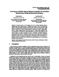
Figure 1: The genome and the structure of a single genetic element. Each element consists of a type field, a sign field, and a sequence of N real values used to determine affinity to other elements (N = 2 was used in this paper).

Genomes are composed of a list of genetic elements. Several genetic elements form a regulatory unit, which corresponds to a node in a regulatory network. Genetic elements fall into three classes. “Genes” are elements that code products (transcription factors, TFs). Products can bind to “promoters” (a generic term for regulatory regions). “Special elements” code for either external inputs or outputs of the regulatory network. The genome is parsed sequentially and divided into regulatory units whenever a series of promoters followed by a series of genes is found (Fig. 1). In other words, each regulatory unit can be composed of one or several regulatory elements and one of several genes encoding TFs. In the next step, special elements are assigned to inputs or outputs, according to their type. The first special element of type one is assigned to the first input, and so on. The same goes for special elements of type two and the outputs. The number of inputs/outputs depends on the particular experiment. If

Each genetic element in our system encodes a point in N dimensional space (Fig. 1). This allows to calculate productpromoter affinity, based on the Euclidean distance between these points (the affinity is high when the distance is small). If the distance is larger than a cut-off value, there is no affinity. This prevents full connectivity in the network. The product of sign fields of the two elements determines the sign of the connection (which can be activatory or inhibitory). The coordinates coded in genetic elements can mutate, so as the genomes evolve, the points in N -dimensional space that correspond to the elements approach one another or move away. Neutral mutations result in a random walk in this space, so only selection limits spreading of the points over time. The activation of a promoter is a sum of the concentration of all products that bind to it, weighted by their affinities. Promoters in our systems can be either additive or multiplicative. The presence of a multiplicative promoter in a regulatory unit results in a strict requirement for the presence of a binding product, otherwise the unit is not expressed. To compute expression of a given regulatory unit, the sum of activations of its additive promoters is multiplied by the activation of its every multiplicative promoter. The result (A) allows to calculate the synthesis/degradation rate of all products in a given regulatory unit: dL dt = fA (A) − L, where L 2 is the current concentration, and fA (A) = 1+e−(A−1) . This sigmoid function can give positive or negative values. The concentration will increase if synthesis rate is higher than that of spontaneous degradation. Otherwise, the degradation will be slowed down or indeed increased (when the fA (A) is negative). Fig. 2 provides an overview of the time scale of spontaneous product degradation in our system. Special elements in our system, as any other genetic elements, are associated with points in N -dimensional abstract space. If a particular special element corresponds to an input, it means that the concentration of this artificial chemical substance is driven externally. Apart from that, the sub-

Proc. of the Alife XII Conference, Odense, Denmark, 2010

204

The model Genome and genetic elements

0 10

30

50

Figure 2: Time scale of product degradation. The product concentrations are in the range < 0, 1 >. The intrinsic degradation can increase if a gene is negatively regulated.

runs were terminated after no improvement over the last 500 generations was detected (typically, after 2500 − 10000 generations). Shorter runs would often indicate lower evolvability (genetic algorithm stuck in a local optimum rather than continuously improving the network).

Fitness function stance behaves as any other TF in the system and regulates other genes, with one exception: it cannot directly control the output node of the network. Although this could be beneficial for some problems, we decided to prevent trivial solutions by requiring all signals to be processed by at least one internal node. For all the experiments presented here, at least one external special substance was provided in this manner, having a fixed concentration of “1”. This is because it is necessary to have a substance with a non zero concentration to start the GRN activity. For networks evolved to react to changing concentrations of external substances, additional input elements were provided. If an input element can be seen as a regulatory unit with one gene and zero promoters (its concentration is driven externally), an output element is treated as a regulatory unit with only one promoter and a gene that does not code for a TF. The concentration of the output gene product is thus a clearly defined exit point for all information processing in the system, even though the fact that connections between the output node and the internal nodes are not permitted is expected to have a minor detrimental effect on evolvability. Only one output was allowed.

The target for evolution was to obtain desired expression patterns as a response to particular input signals. A straightforward approach would be to aim to minimize the difference between theP desired (dt ) and obtained (ot ) expression levels over time: |ot − dt |. However, this often lead us to t

unsatisfying, suboptimal solutions. This is because many of the target patterns require keeping output product expression at 0 for some time, so lack of expression during the whole time results in higher fitness than, for example, a pattern that is shifted but otherwise correct. Once such trivial solution is reached, little can be improved by evolution: there is no regulation that can be fine tuned. We alleviated this problem by including the terms that give higher weight for correctly expressing output product when its concentration is expected to be higher and for the correct number of oscillations in periodic expression patterns: L X t=p

|ot − dt |(1 + kdt )

1 1+S

(1)

Genetic operators can act on the level of single elements or multiple elements. On the level of single elements, particular fields can be mutated, changing element type, sign bit, or disturbing the coordinates of an associated point in space. Single or multiple elements can be deleted or duplicated. A series of duplications and deletions can lead to changes in the order of the elements. Changes in the order of promoters within a regulatory unit are neutral, the same goes for the changes in the order of genes. Changing the order of regulatory units does not lead to changes in the topology of the network so it is also neutral. Any type change is permitted. In particular, new input and output elements can be created from other elements (genes, promoters) when the type field of an element is changed by mutation. Type mutations can in principle lead to the loss of inputs or outputs. Obviously, in the experiments described here, such loss would be highly deleterious. The results shown in this work were obtained using a fairly standard genetic algorithm with a population size of 300, elitism, tournament selection, and multipoint crossover for sexual reproduction (for 30% of the individuals in each generation). Evolutionary runs were initiated with individuals consisting of 5 randomly created regulatory units. The

where L is the number of GRN simulation steps (between 600 and 1000 clock ticks, depending on the experiment), and k increases the weight of properly expressed high concentrations (k = 2 was used). Parameter p (“propagation time”) allows to set the number of simulation steps after which the activity of the output is evaluated. Because some time is needed to build up TF concentrations, it is not reasonable to penalize the network whatever its activity during this time. Propagation time was set to 50 clock ticks: this is a rough estimate of the time needed to form a response. The last term promotes evolution of oscillatory patterns. S was set to 1 when the desired number of oscillations was obtained or to 0 when there was no oscillations or too many (more than twice the desired number). Imperfect matches resulted in intermediate values. To keep the matters simple, the number of events when the expression crosses the level of 0.5 was counted (the events when dt−10 < 0.5 and dt ≥ 0.5 or dt−10 ≥ 0.5 and dt < 0.5). The minimum distance between countable events was set to 10 clock ticks to prevent trivial fluctuations around 0.5. Inclusion of this term in the error function promotes the correct number of oscillations from the very beginning, even if not timed correctly. Calculated error was further normalized, so that a perfect match in expression pattern would result in individual scoring 0 and the worst possible would score 1. For experiments where multiple training pairs were used, the final fitness would be an average of every test case.

Proc. of the Alife XII Conference, Odense, Denmark, 2010

205

Genetic algorithm

OUT

0

100

200

300

400

500

600

Figure 3: Behaviour of an evolved network that gives a sine wave expression pattern lasting for five periods (the best network in 10 runs); dashed line: the desired response.

Results Internally induced oscillations We have first analysed if our system allows for evolution of networks in which an output product level oscillates. Oscillating gene expression has been previously investigated in somewhat similar artificial GRN models (Kuo et al., 2004; Knabe et al., 2006). This task can be made easier by providing the network with a periodically changing input of the same frequency as the target. However, no such input was made available in our experiments: the only external signal was a special product with a constant maximum concentration, so the obtained dynamics was internally induced. It proved very easy to evolve oscillating expression with almost perfect match to the target pattern (sine waveforms) in a large range of frequencies and amplitudes. The oscillations were stable: they persisted also when the number of simulation steps was increased beyond the network lifespan used at the evaluation stage during evolution. In a more challenging task, the target was a sine wave starting at a certain time point and ending after 5 periods. The oscillations in the best networks found in 9 independent runs out of 10 had proper frequency but did not terminate. Only in one run a good solution was obtained (Fig. 3), even though the phase of the output signal does not match the target phase. This is penalized by the error function, but the solution is rewarded because the number of pulses is correct (Eq. 1). Perhaps the difference in fitness between a solution in which oscillations terminate and a solution in which they do not is too small and this is why most runs got stuck in a local minimum. If so, simple extension of the lifespan beyond 600 clock ticks would improve evolvability.

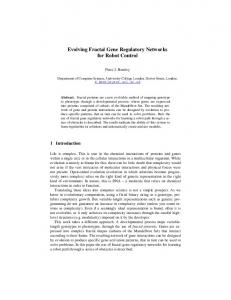
behaviour of the best network obtained. The solutions were general: intermediate frequencies were also doubled. Even very low frequencies posed no problem (Fig. 4c, note that the time scale is different in different panels). Indeed, for the best individuals we were not able to find a frequency that would be too low to elicit the proper response. Generalizing to frequencies above the range in the training set proved more challenging. The networks did not behave as desired when the frequency was increased more than about 40% (Fig. 4d); interestingly, the best GRN in an experiment in which the frequencies in the training examples were two times lower had about the same relative upper limit. The behaviour of the best GRN was tested using an input pattern in which frequency changed multiple times (in the training patterns, frequency was constant). The network showed correct behaviour: matching the output frequency to the input frequency (not shown). However, less general solutions were obtained in some runs: these GRNs would lock their outputs to the frequency present at the beginning of a complex input pattern. It is difficult to analyse how exactly the output of the best GRN is calculated because of the high density of the networks, about 0.5-0.6 (30-50 regulatory units linked with about 1000 edges, encoded with roughly 250 genetic elements). However, a hint on inner mechanics can be obtained by replacing the sinusoidal input with a trapezoid waveform and changing its duty cycle. It can be seen (Fig. 4e) that a spike of the output expression is generated for each raising and each falling edge in the input. This suggests that the poor generalization for higher frequencies may result from the fact that the rate of output product accumulation and degradation is adjusted to the rates used in the training set. If so, concentrations will increase and decrease too fast when the frequency is low; indeed, this can be observed in Fig. 4c).

Low pass frequency filter

Apart from the task described above, all the others involved processing continuously changing input signals. In the first such task, the networks were expected to double the frequency of the input oscillations (sine wave). Three training inputs were provided at the evaluation stage in the GA: two sinusoidal curves with different frequencies and an input in which the signal was kept at 0 (requiring an empty response). The “no signal” input was included to facilitate emergence of solutions that are active only when external signal is present. In 10 out of 10 runs the evolved networks displayed the correct behaviour for the training set. Fig. 4ab shows the

Filtering input frequency is a problem well suited for regulatory networks: limited speed of accumulation and degradation of TFs will work as an RC circuit. In this task the networks were expected to regenerate in the output the frequency of the input sinusoid, but only if this frequency was below a certain threshold. Five inputs were provided in the training set: two with frequencies below the threshold, two with frequencies above it, plus the “no signal” input which was again expected to give no output signal. It was easy to obtain networks with correct behaviour that generalized for frequencies higher and lower than those in the training set. However, providing these network with a sum of two sinusoids with only one frequency below the threshold (an example of such input is provided in Fig. 5cd) would result in no output signal. This suggests that these networks simply detected the high rising slope in the input and blocked the output if it was too high.

Proc. of the Alife XII Conference, Odense, Denmark, 2010

206

Doubling the input frequency

IN

IN

OUT

OUT

(a)

(a) 0

200

400

600

800

1000

IN

0

200

400

600

800

0

1000

200

400

600

800

1000

IN

OUT

0

200

400

600

800

1000

200

400

600

800

1000

200

400

600

800

1000

200

400

600

800

1000

200

400

600

800

1000

OUT

(b)

(b) 0

200

400

600

800

1000

0

200

400

600

800

0

1000

200

400

600

800

1000

IN IN

0 OUT

(c)

OUT

(c) 0 0

5000

10000

15000

IN

0

5000

10000

200

400

600

800

1000

IN

15000

0 OUT

(d)

OUT

(d) 0 0

200

400

600

800

1000

IN

0

200

400

600

800

200

400

600

800

1000

0

1000

OUT

IN

OUT

(e)

(e) 0

200

400

600

800

1000

0

200

400

600

800

1000

Figure 4: Behaviour of the network evolved to double the frequency of the input signals (the best solution in 10 evolutionary runs, obtained after 6191 generations): (ab) the response for the inputs in the training set (the correct response for the “no signal” input is not shown), (c) this network behaves correctly for an input with much lower frequency than in the training set (note that the time scale was changed), but fails to generalize for inputs with slightly higher frequency (d), the response for the signal in panel (e) hints on the way in which the output is calculated. Dashed lines in (a-d): the desired ideal response. .

0

200

400

600

800

1000

IN

0 OUT

(f) 0

500 1000

2000

3000

0

500 1000

2000

3000

Figure 5: Behaviour of a GRN (the best individual in 10 evolutionary runs, obtained in generation 8839) acting as a low pass filter for the inputs in the training set (a-d; only half of the training examples is shown) and the inputs for which the network was not evaluated during the genetic algorithm (ef). The dashed lines correspond to the desired response.

In the tasks described above, obtaining the solution did not require the explicit memory of the input signal. This is not the case for the task in which the networks were expected to respond with a square pulse twice the length of the square pulse in the input after 50 simulation steps. Three input patterns plus the “no signal” input were used in the training set

(Fig. 6a-c). Good solutions were obtained in all 10 evolutionary runs. The best network (Fig. 6a-c) behaved correctly also when the square pulses in the inputs occurred at different times than in the inputs used in the training set. It also behaved as expected when the input pattern consisted of subsequent square pulses. Good generalization was observed for pulses with other (intermediate) lengths than the pulses in the training set. Pulses up to 50% shorter (Fig. 6d-f) than the shortest training pulse gave the desired response, but pulses longer than the longest training pulse gave responses shorter than desired (Fig. 6e), exposing leaky nature of the GRN-based memory. When the pulses in the input had half the height of those in the training set (Fig. 6f), the length of the output pulse would be close to that of the input pulse. This suggests that the network acts as a simple integrator (e.g. by slowly building up some concentrations) instead of reacting to raising and falling edge of the input signal like frequency doubling networks. When the networks were required to output a square pulse with doubled length after 300 time steps instead of 50, the behaviours were less accurate, though proper generalization was still observed. The average value of error function (considering only the best individuals in each independent run

Proc. of the Alife XII Conference, Odense, Denmark, 2010

207

To improve generality of the solutions, we have added such inputs to the training set, requiring the network to filter out just the higher frequency component. Fig. 5e shows the behaviour of a network that correctly if imperfectly filters the high frequency component even for an input not in the training set. This network shows correct behaviour also when another input not in the training set was used (Fig. 5f), adjusting “on the fly” the output signal to the changing frequency in the input. However, such behaviour was observed for the best GRNs only in some of the runs. The best networks in other runs failed to generalize and locked to the frequency present at the beginning of a complex input pattern. This is similar to what was observed in the previous task.

Doubling the pulse length

IN

IN

OUT

OUT

(a)

(a) 0

200

400

600

800

1000

IN

0

200

400

600

800

0

1000

200

400

600

800

IN

OUT

0

200

400

600

800

200

400

600

800

200

400

600

800

200

400

600

800

OUT

(b)

(b) 0

200

400

600

800

1000

IN

0

200

400

600

800

0

1000

200

400

600

800

IN

OUT

0 OUT

(c)

(c) 0

200

400

600

800

1000

IN

0

200

400

600

800

0

1000

200

400

600

800

IN

OUT

0

OUT

(d)

(d) 0

200

400

600

800

1000

IN

0

200

400

600

800

1000

OUT

(e) 0

200

400

600

800

1000

IN

0

200

400

600

800

1000

200

400

600

800

1000

OUT

(f) 0

200

400

600

800

1000

0

Figure 6: Behaviour of the network evolved to double the input pulse length (the best individual in 10 evolutionary runs, obtained in generation 7295): (a-c) the responses for the inputs in the training set (the response to the “no signal” input was not shown) and (d-f) for the inputs used when testing for generality. Dashed lines correspond to the desired ideal response.

out of 10) was worse: 0.054 for 300 steps vs. 0.017 for 50. The values were also more variable (standard deviation was 0.027 and 0.002, respectively). This further demonstrates the leaky nature of evolved GRN-based memories: the longer the networks have to store the information, the more degraded it becomes.

Doubling the number of input pulses From the biological point of view, the GRNs discussed thus far could be seen as responding to continuously raising and falling concentration of chemical substance (pulses in the input). What was relevant was the frequency or the length of the pulses. In the next two problems, the number of pulses will be important. The first task, doubling the number of pulses, can be seen as more difficult than the previous problem. The response still requires performing multiplication, but the number of subsequent pulses needs to be counted, not the pulse length. Fig. 7a-c shows that the best network obtained in 10 runs correctly doubles the number of pulses in the training set inputs when this number is one or two. The solution when the expected number of subsequent oscillations is six is almost correct. However, the generalization is imperfect: seven in-

Proc. of the Alife XII Conference, Odense, Denmark, 2010

0

200

400

600

800

0

Figure 7: Behaviour of a GRN that doubles the number of spikes (the best individual in 10 evolutionary runs, obtained in generation 2794): (a-c) the network behaves correctly or almost correctly for the training set input, but (d) responds with less spikes than expected when the generality of the solution is tested with a higher number of spikes in the input.

stead of eight pulses for four pulses in the input (Fig. 7d), a response shorter than expected. This reminds the behaviour of GRNs evolved to double pulse lengths when presented with input pulses longer than the longest in the training set.

Integrating information from two separate signals: counting pulses The experiment described above indicates that a task that involves processing concentration pulses allows to approach the limits of our system in terms of searching for networks with desired signal processing properties. To make the task even more difficult, the networks were required to process signals from two inputs instead of one. The task was to respond with the number of output pulses equal to the number of pulses on both inputs within a certain time window (see Fig. 8a-e for the training set). No response was expected when no input pulses were present in the pattern. Fig. 8 shows the behaviour of the best GRN in 10 runs. This network is able not only to count correctly the pulses in the training set but is also general enough to work in a continuous manner (Fig. 8f).

Modifying the system time step Product accumulation and degradation in our system is simulated in discrete steps. Changes in concentration are computed with every iteration with a time step dt = 0.1. The step size is a compromise between accuracy and computation cost. In principle, it would be possible for some of the evolved networks to exploit inaccuracies that would occur if some concentrations were to change rapidly due to overregulation and wrongly chosen dt. To test if this is an issue

208

IN1

IN2

OUT

IN1

OUT

(a) 0

100

300

500

IN1

0

100

300

500 0

IN2

100

300

500

(b) 0

100

300

500

IN1

0

0

200

400

600

800

1000

0

200

400

600

800

1000

OUT

100

300

500 0

IN2

100

300

500

300

500

OUT

Figure 9: The best individual obtained in 10 evolutionary runs using a modified model in which product built-up and degradation is not simulated (response to one of the training signals is shown).

(c) 0

100

300

500

IN1

0

100

300

500 0

IN2

100

OUT

(d) 0

100

300

500

IN1

0

100

300

500 0

IN2

100

300

500

300

500

OUT

(e) 0

100

300

500

IN1

0

100

300

500 0

IN2

100

the input frequency. The behaviour of the best individual for a non-continuous model Fig. 9 can be compared with that observed in Fig. 4. Even though a good solution was found, the evolvability itself was clearly worse. Average error for 10 runs with a modified model was 0.075 (sd: 0.025). For the model with continuous TF synthesis/degradation the error was 0.026 (sd: 0.005).

Discussion

OUT

(f)

In the GRN model used here the TF concentration at a particular time point is determined by its synthesis and degradation rates and its concentration at the previous time step. In order to test if this GRN property is important for signal processing tasks, we have modified the model so that the gene expression was determined only by the activation of associated promoters in the previous time step. More precisely, the function fA (A), instead of being treated as current product synthesis level (with the range < −1, 1 >), would be shifted right and scaled to < 0, 1 > so that it could be treated as a new expression level for the given time step. This allows genes to change its activity instantly. In this model GRNs behave similarly to recurrent networks of perceptron-like neurons (similar regulatory networks were used by us Joachimczak and Wr´obel (2008) and other researchers, e.g. Eggenberger (1997). To see if this change affects evolvability, we compared the average fitness for the best individuals in 10 runs using the problem of doubling

The goal of this work was to investigate in a qualitative and exploratory manner the possibility to evolve artificial GRN that can generate or process continuous signals provided as externally driven concentrations of chemical substances. We have tested if the way we have formulated the encoding of the structure of the networks in a linear genome and the genetic algorithm allows for evolvability in several problems of various difficulty. Several attempts have been made previously by us and other researchers to employ artificial GRNs for various tasks (such as development). It is thus interesting to investigate what kind of information processing can be performed by single cells equipped with such networks. In general, given enough simulation steps, artificial GRNs can be expected to be similar to perceptron-like artificial neural networks (ANNs) with recurrent connections in terms of computational properties, even though the biological inspiration is different. Perhaps the most important difference between the GRN model used here and commonly used ANN models is that here the state of a regulatory node, represented by the concentration of associated products (transcriptional factors) is influenced by the rate of product synthesis and degradation. This limits the response time of the network. On the other hand, smoothness of gene expression provides an advantage for generating gradually changing outputs, such as sine waves (compare Fig. 4b and Fig. 9). One could also expect that such inherent dynamics of each node could be exploited by biological GRNs when dealing with noisy external signals and with the inherent noisiness of gene expression itself. Obviously, “no free lunch” theorem applies: GRNs may provide an advantage in a certain class of problems, but one should not expect them to universally outperform other approaches. In particular, computations that required counting pulses of input substance concentration proved more difficult than other tasks (which also involved simple mathematical cal-

Proc. of the Alife XII Conference, Odense, Denmark, 2010

209

0

500

1000

1500

0

500

1000

1500 0

500

1000

1500

Figure 8: Behaviour of the GRN evolved to count the pulses in two inputs (the best individual in 10 evolutionary runs, obtained in generation 2168): (a-e) the network gives an expected output for the the inputs in the training set and the (f) inputs used to test for generality.

we decreased dt by an order of magnitude and increased 10fold the number of simulation steps. This increased simulation accuracy but did not affect the behaviour of any of the networks discussed above.

The importance of continuous TF accumulation/degradation

culations and memory). Processing information encoded in pulses is superficially similar to information processing in spiking neural networks. However, in GRN-based systems the pulses result from simulated product accumulation followed by degradation not by simulation of ion transport through the membrane, often extremely simplified (so that a spike results when a threshold potential is reached). It is reasonable to assume that this kind of information encoding is far from optimal for processing signals with regulatory networks. In other words, problems that require pulse counting can help to find the limit of what can be evolved using GRNbased systems such as ours. Introducing more realistic molecular dynamics could make evolving artificial GRN models a useful tool for obtaining synthetic regulatory networks (see e.g. Friedland et al., 2009; Elowitz and Leibler, 2000). Such networks might find applications for example in intelligent delivery of therapeutic chemical substances (small molecules, proteins, regulatory RNAs), regulated by external signals. Artificial evolution would allow to design such networks and optimize them by various criteria, such as the number of regulatory elements and genes or robustness to noise. The evolvability in signal processing tasks could be also improved by changes in the error function or reformulation of the tasks themselves. For example, it would probably help to look for the best match of the output expression pattern within a certain range of allowable response times instead of requiring the pattern to appear after a predefined response delay. Although it would be very interesting to further explore the areas hinted above, the next step in our work will be to investigate the statistical properties of evolving artificial GRNs and to employ the model described here in other control problems, for example, animat navigation.

Acknowledgements This work was supported by the Polish Ministry of Science and Education (project N519 384236). The computational resources used in this work were obtained thanks also to the support of the project N303 291234, the Tri-city Academic Computer Centre (TASK) and the Interdisciplinary Centre for Molecular and Mathematical Modelling (ICM, University of Warsaw; project G33-8).

References Andersen, T., Newman, R., and Otter, T. (2009). Shape homeostasis in virtual embryos. Artificial Life, 15(2):161–183. Banzhaf, W. (2003). On the dynamics of an artificial regulatory network. In Proceedings of the 7th European Conference (ECAL 2003) Dortmund, Germany, September 14-17, 2003, Lecture Notes in Artificial Intelligence, pages 217–227. Springer Berlin / Heidelberg.

in Developmental Systems in the Genetic and Evolutionary Computation Conference (GECCO 2004). Eggenberger, P. (1997). Evolving morphologies of simulated 3D organisms based on differential gene expression. In Proceedings of the Fourth European Conference on Artificial Life, pages 205–213, Cambridge, MA. MIT Press. Elowitz, M. B. and Leibler, S. (2000). A synthetic oscillatory network of transcriptional regulators. Nature, 403(6767):335– 338. Friedland, A. E., Lu, T. K., Wang, X., Shi, D., Church, G., and Collins, J. J. (2009). Synthetic gene networks that count. Science, 324(5931):1199–1202. Joachimczak, M. and Wr´obel, B. (2008). Evo-devo in silico: a model of a gene network regulating multicellular development in 3D space with artificial physics. In Artificial Life XI: Proceedings of the Eleventh International Conference on the Simulation and Synthesis of Living Systems, pages 297–304. MIT Press, Cambridge, MA. Joachimczak, M. and Wr´obel, B. (2009). Evolution of the morphology and patterning of artificial embryos: scaling the tricolour problem to the third dimension. In Proceedings of 10th European Conference on Artificial Life (ECAL 2009). Springer. Knabe, J. F., Nehaniv, C. L., Schilstra, M. J., and Quick, T. (2006). Evolving biological clocks using genetic regulatory networks. In Artificial Life X: Proceedings of the Tenth International Conference on the Simulation and Synthesis of Living Systems, pages 15–21. MIT Press/Bradford Books. Kuo, D., P., Banzhaf, W., and Leier, A. (2006). Network topology and the evolution of dynamics in an artificial genetic regulatory network model created by whole genome duplication and divergence. BioSystems, 85(3):177–200. Kuo, D. P., Leier, A., and Banzhaf, W. (2004). Evolving dynamics in an artificial regulatory network model. In Parallel Problem Solving from Nature - PPSN VIII, volume 3242 of Lecture Notes in Computer Science, pages 571–580. Springer Berlin / Heidelberg. Nicolau, M. and Schoenauer, M. (2009). On the evolution of scale-free topologies with a gene regulatory network model. BioSystems, 98(3):137–148. Quick, T., Nehaniv, C. L., Dautenhahn, K., and Roberts, G. (2003). Evolving embodied genetic regulatory network-driven control systems. In Advances in Artificial Life, pages 266–277. Reil, T. (1999). Dynamics of gene expression in an artificial genome - implications for biological and artificial ontogeny. In Proceedings of the 5th European Conference on Artificial Life, volume 1674 of Lecture Notes In Computer Science, pages 457–466, London, UK. Springer-Verlag. Schramm, L., Jin, Y., and Sendhoff, B. (2009). Emerged coupling of motor control and morphological development in evolution of multi-cellular animats. In Kampis, G. and Szathm´ary, E., editors, Proceedings of 10th European Conference on Artificial Life (ECAL 2009). Springer.

Bentley, P. J. (2004). Adaptive fractal gene regulatory networks for robot control. In Workshop on Regeneration and Learning

Taylor, T. (2004). A genetic regulatory network-inspired real-time controller for a group of underwater robots. In Proceedings of the Eighth Conference on Intelligent Autonomous Systems (IAS-8), pages 403–412.

Proc. of the Alife XII Conference, Odense, Denmark, 2010

210