for matrix product, Gaussian elimination, and transitive closure. ... Parallel execution of uniform recurrence equations has been studied extensively, from at least.
Processor-Time-Optimal Systolic Arrays Peter Cappello, Omer E�gecio�glu, and Chris Scheiman Abstract Minimizing the amount of time and number of processors needed to perform an application reduces the application's fabrication cost and operation costs. A directed acyclic graph (dag) model of algorithms is used to de ne a time-minimal schedule and a processor-time-minimal schedule. We present a technique for nding a lower bound on the number of processors needed to achieve a given schedule of an algorithm. The application of this technique is illustrated with a tensor product computation. We then apply the technique to the free schedule of algorithms for matrix product, Gaussian elimination, and transitive closure. For each, we provide a timeminimal processor schedule that meets these processor lower bounds, including the one for tensor product.
Keywords: algebraic path problem, dag, Diophantine equation, Gaussian elimination, matrix product, optimal, systolic array, tensor product, transitive closure.
1
Introduction
We consider regular array computations, often referred to as systems of uniform recurrence equations [26]. Parallel execution of uniform recurrence equations has been studied extensively, from at least as far back as 1966 (e.g., [25, 31, 29, 7, 37, 9, 10, 38, 39, 13]). In such computations, the tasks to be computed are viewed as the nodes of a directed acyclic graph, where the data dependencies are represented as arcs. Given a dag G = (N; A), a multiprocessor schedule assigns node v for processing during step � (v) on processor �(v). A valid multiprocessor schedule is subject to two constraints:
Causality: A node can be computed only when its children have been computed at previous steps. Non-con ict: A processor cannot compute 2 di�erent nodes during the same time step. 1
In what follows, we refer to a valid schedule simply as a schedule. A time-minimal schedule for an algorithm completes in S steps, where S is the number of nodes on a longest path in the dag. A time-minimal schedule exposes an algorithm's maximum parallelism. That is, it bounds the number of time steps the algorithm needs, when in nitely many processors may be used. A processor-time minimal schedule is a time-minimal schedule that uses as few processors as any time-minimal schedule for the algorithm. Although only one of many performance measures, processor-time-minimality is useful because it measures the minimum processors needed to extract the maximum parallelism from a dag. Being machine-independent, it is a more fundamental measure than those that depend on a particular machine or architecture. This view prompted several researchers to investigate processortime-minimal schedules for families of dags. Processor-time-minimal systolic arrays are easy to devise, in an ad hoc manner, for 2D systolic algorithms. This apparently is not the case for 3D systolic algorithms. There have been several publications regarding processor-time-minimal systolic arrays for fundamental 3D algorithms. Processor-time-minimal schedules for various fundamental problems have been proposed in the literature: Scheiman and Cappello [8, 5, 47, 44] examine the dag family for matrix product; Louka and Tchuente [33] examine the dag family for Gauss-Jordan elimination; Scheiman and Cappello [45, 46] examine the dag family for transitive closure; Benaini and Robert [3, 2] examine the dag families for the algebraic path problem and Gaussian elimination. Each of the algorithms listed in Table 1 has the property that, in its dag representation, every node is on a longest path: Its free schedule is its only time-minimal schedule. A processor lower bound for achieving it is thus a processor lower bound for achieving maximum parallelism with the algorithm. Table 1: Some 3D algorithms for which processor-time-minimal systolic arrays are known.
Algorithm
Citation
Algebraic Path Problem Gauss-Jordan elimination Gaussian elimination Matrix product Transitive closure Tensor product
[3] [33] [3] [8, 5] [45] this article 2
Time Processors 5n ? 2 n =3 + O(n) 2
4n 3n ? 1 3n ? 2 5n ? 4 4n ? 3
5n =18 + O(n) n =4 + O(n) d3n =4e dn =3e (2n + n)=3 2
2
2
2
2
Clauss, Mongenet, and Perrin [11] developed a set of mathematical tools to help nd a processortime-minimal multiprocessor array for a given dag. Another approach to a general solution has been reported by Wong and Delosme [57, 58], and Shang and Fortes [48]. They present methods for obtaining optimal linear schedules. That is, their processor arrays may be suboptimal, but they get the best linear schedule possible. Darte, Khachiyan, and Robert [13] show that such schedules are close to optimal, even when the constraint of linearity is relaxed. Geometric/combinatorial formulations of a dag's task domain have been used in various contexts in parallel algorithm design as well (e.g., [25, 26, 31, 37, 38, 18, 17, 39, 11, 48, 54, 58]; see Fortes, Fu, and Wah [16] for a survey of systolic/array algorithm formulations.) In x2, we present an algorithm for nding a lower bound on the number of processors needed to achieve a given schedule of an algorithm. The application of this technique is illustrated with a tensor product computation. Then, in x3, we apply the technique to the free schedule of algorithms for matrix product, Gaussian elimination, and transitive closure. For each, we provide a compatible processor schedule that meets these processor lower bounds (i.e., a processor-time-minimal schedule) including the one for tensor product. We nish with some general conclusions and mention some open problems. One strength of our approach centers around the word algorithm: we are nding processor lower bounds not just for a particular dag, but for a linearly parameterized family of dags, representing the in nitely many problem sizes for which the algorithm works. Thus, the processor lower bound is not a number but a polynomial (or nite set of polynomials) in the linear parameter used to express di�erent problem sizes. The formula then can be used to optimize the implementation of the algorithm, not just a particular execution of it. The processor lower bounds are produced by:
� formulating the problem as nding, for a particular time step, the number of processors needed by that time step as a formula for the number of integer points in a convex polyhedron,
� representing this set of points as the set of solutions to a linearly parameterized set of linear Diophantine equations,
� computing a generating function for the number of such solutions, � deriving a formula from the generating function. 3
The ability to compute formulae for the number of solutions to a linearly parameterized set of linear Diophantine equations has other applications for nested loops [12], such as nding the number of instructions executed, the number of memory locations touched, and the number of I/O operations. The strength of our algorithm|its ability to produce formulae|comes, of course, with a price: The computational complexity of the algorithm is exponential in the size of the input (the number of bits in the coe�cients of the system of Diophantine equations). The algorithm's complexity however is quite reasonable given the complexity of the problem: Determining if there are any integer solutions to the system of Diophantine equations is NP-complete [19]; we produce a formula for the number of such solutions. Clauss and Loechner independently developed an algorithm for the problem based on Ehrhart polynomials. In [12], they sketch an algorithm for the problem, using the \polyhedral library" of Wilde [56].
2
Processor Lower Bounds
We present a general and uniform technique for deriving lower bounds: Given a parametrized dag family and a correspondingly parametrized linear schedule, we compute a formula for a lower bound on the number of processors required by the schedule.
This is much more general than the analysis of an optimal schedule for a given speci c dag. The lower bounds obtained are good; we know of no dag treatable by this method for which the lower bounds are not also upper bounds. We believe this to be the rst reported algorithm and its implementation for automatically generating such formulae. The nodes of the dag typically can be viewed as lattice points in a convex polyhedron. Adding to these constraints the linear constraint imposed by the schedule itself results in a linear Diophantine system of the form az = nb + c ; (1) where the matrix a and the vectors b and c are integral, but not necessarily non-negative. The number dn of solutions in non-negative integers z = [z ; z ; : : : ; zs ]t to this linear system is a lower 1
4
2
bound for the number of processors required when the dag corresponds to parameter n. Our algorithm produces (symbolically) the generating function for the sequence dn , and from the generating function, a formula for the numbers dn . We do not make use of any special properties of the system that re ects the fact that it comes from a dag. Thus in (1), a can be taken to be an arbitrary r � s integral matrix, and b and c arbitrary integral vectors of length r. As such we actually solve a more P general combinatorial problem of constructing the generating function n� dn tn , and a formula for dn given a matrix a and vectors b and c, for which the lower bound computation is a special case. There is a large body of literature concerning lattice points in convex polytopes and numerous interesting results: see for example Stanley [50] for Ehrhart polynomials (Clauss and Loechner [12] use these), and Sturmfels [51, 52] for vector partitions and other mathematical treatments. Our results are based mainly on MacMahon [34, 36], and Stanley [49]. 0
2.1 Example: Tensor product We examine the dag family for the 4D mesh: the n � n � n � n directed mesh. This family is fundamental, representing a communication-localized version of the standard algorithm for Tensor product (also known as Kronecker product). The Tensor product is used in many mathematical computations, including multivariable spline blending and image processing [20], multivariable approximation algorithms (used in graphics, optics, and topography) [28], as well as many recursive algorithms [27]. The Tensor product of an n � m matrix A and a matrix B is: 2
a B a B : : : a mB 6 6 A B = 64 : : : an B an B : : : anm B 11
12
1
2
1
3 7 7 7 5
The 4D mesh also represents other algorithms, such as the least common subsequence problem [23, 22], for 4 strings, and matrix comparison (an extension of tuple comparison [24]). An example dag is shown in Figure 1, for n = 3.
2.1.1 The dag The 4D mesh can be de ned as follows. Gn = (Nn ; An ), where
� Nn = f(i; j; k; l) j 0 � i; j; k; l � n ? 1g. 5
� An = f[(i; j; k; l); (i0; j 0 ; k0 ; l0 )] j(i; j; k; l) 2 Nn ; (i0 ; j 0 ; k0 ; l0) 2 Nn and exactly 1 of the following conditions holds:
1. i0 = i + 1; j 0 = j; k0 = k; l0 = l; 2. j 0 = j + 1; i0 = i; k0 = k; l0 = l; 3. k0 = k + 1; i0 = i; j 0 = j; l0 = l; 4. l0 = l + 1; i0 = i; j 0 = j; k0 = k:g
2.1.2 The parametric linear Diophantine system of equations The computational nodes are de ned by non-negative integral 4-tuples (i; j; k; l) satisfying
i j k l
� � � �
n?1 n?1 n?1 n?1 :
Introducing nonnegative integral slack variables s ; s ; s ; s � 0, we obtain the equivalent linear Diophantine system describing the computational nodes as 1
i
j
+s
k
2
3
4
1
+s
2
l
+s
3
+s
4
= = = =
n?1 n?1 n?1 n?1
A linear schedule for the corresponding dag is given by � (i; j; k; l) = i + j + k + l +1. For this problem � ranges from 1 to 4n ? 3. The computational nodes about halfway through the completion of the schedule satisfy the additional constraint
i + j + k + l = 2n ? 2
6
6
7
5
8
6
4
7
5
6
5
6
4
7
5
3
6
4
5
4
5
3
6
4
2
5
3
5
4
6
4
7
5
3
6
4
5
4
5
3
6
4
2
5
3
4
3
4
2
5
3
1
4
2
4
3
5
3
6
4
2
5
3
4
3
4
2
5
3
1
4
2
3
2
3
1
4
2
0
1
3 2
Figure 1: The 4-dimensional cubical mesh, for n = 3.
7
Adding this constraint we obtain the augmented Diophantine system
i +j +k +l i +s j +s k +s l +s 1
2
3
4
= = = = =
2n ? 2 n?1 n?1 n?1 n?1
(2)
Therefore, a lower bound for the number of processors needed for the Tensor Product problem is the number of solutions to (2). The corresponding Diophantine system is az = nb + c where 2
a=
6 6 6 6 6 6 6 6 6 4
1 1 0 0 0
1 0 1 0 0
1 0 0 1 0
1 0 0 0 1
0 1 0 0 0
0 0 1 0 0
0 0 0 1 0
3
07 0 777 0 777 ; 0 775 1
2
b=
6 6 6 6 6 6 6 6 6 4
3
27 1 777 1 777 ; 1 775 1
2
?2 6 6 6 ?1 6 c = 666 ?1 6 6 ?1 4 ?1
3 7 7 7 7 7 7 7 7 7 5
(3)
2.1.3 The Mathematica program input & output Once the Mathematica program DiophantineGF.m for this computation has been loaded by the command