Product-based Neural Networks for User Response Prediction - arXiv

Product-based Neural Networks for User Response Prediction

arXiv:1611.00144v1 [cs.LG] 1 Nov 2016

Yanru Qu, Han Cai, Kan Ren, Weinan Zhang, Yong Yu Shanghai Jiao Tong University {kevinqu, hcai, kren, wnzhang, yyu}@apex.sjtu.edu.cn

Abstract—Predicting user responses, such as clicks and conversions, is of great importance and has found its usage in many Web applications including recommender systems, web search and online advertising. The data in those applications is mostly categorical and contains multiple fields; a typical representation is to transform it into a high-dimensional sparse binary feature representation via one-hot encoding. Facing with the extreme sparsity, traditional models may limit their capacity of mining shallow patterns from the data, i.e. low-order feature combinations. Deep models like deep neural networks, on the other hand, cannot be directly applied for the high-dimensional input because of the huge feature space. In this paper, we propose a Product-based Neural Networks (PNN) with an embedding layer to learn a distributed representation of the categorical data, a product layer to capture interactive patterns between interfield categories, and further fully connected layers to explore high-order feature interactions. Our experimental results on two large-scale real-world ad click datasets demonstrate that PNNs consistently outperform the state-of-the-art models on various metrics.

I. I NTRODUCTION Learning and predicting user response now plays a crucial role in many personalization tasks in information retrieval (IR), such as recommender systems, web search and online advertising. The goal of user response prediction is to estimate the probability that the user will provide a predefined positive response, e.g. clicks, purchases etc., in a given context [1]. This predicted probability indicates the user’s interest on the specific item such as a news article, a commercial item or an advertising post, which influences the subsequent decision making such as document ranking [2] and ad bidding [3]. The data collection in these IR tasks is mostly in a multifield categorical form, for example, [Weekday=Tuesday, Gender=Male, City=London], which is normally transformed into high-dimensional sparse binary features via onehot encoding [4]. For example, the three field vectors with one-hot encoding are concatenated as [0, 1, 0, 0, 0, 0, 0] | {z }

[0, 1] | {z}

Weekday=Tuesday Gender=Male

[0, 0, 1, 0, . . . , 0, 0] . | {z } City=London

Many machine learning models, including linear logistic regression [5], non-linear gradient boosting decision trees [4] and factorization machines [6], have been proposed to work on such high-dimensional sparse binary features and produce high quality user response predictions. However, these models

Ying Wen, Jun Wang University College London {ying.wen, j.wang}@cs.ucl.ac.uk

highly depend on feature engineering in order to capture highorder latent patterns [7]. Recently, deep neural networks (DNNs) [8] have shown great capability in classification and regression tasks, including computer vision [9], speech recognition [10] and natural language processing [11]. It is promising to adopt DNNs in user response prediction since DNNs could automatically learn more expressive feature representations and deliver better prediction performance. In order to improve the multi-field categorical data interaction, [12] presented an embedding methodology based on pre-training of a factorization machine. Based on the concatenated embedding vectors, multi-layer perceptrons (MLPs) were built to explore feature interactions. However, the quality of embedding initialization is largely limited by the factorization machine. More importantly, the “add” operations of the perceptron layer might not be useful to explore the interactions of categorical data in multiple fields. Previous work [1], [6] has shown that local dependencies between features from different fields can be effectively explored by feature vector “product” operations instead of “add” operations. To utilize the learning ability of neural networks and mine the latent patterns of data in a more effective way than MLPs, in this paper we propose Product-based Neural Network (PNN) which (i) starts from an embedding layer without pretraining as used in [12], and (ii) builds a product layer based on the embedded feature vectors to model the inter-field feature interactions, and (iii) further distills the high-order feature patterns with fully connected MLPs. We present two types of PNNs, with inner and outer product operations in the product layer, to efficiently model the interactive patterns. We take CTR estimation in online advertising as the working example to explore the learning ability of our PNN model. The extensive experimental results on two large-scale realworld datasets demonstrate the consistent superiority of our model over state-of-the-art user response prediction models [6], [13], [12] on various metrics. II. R ELATED W ORK The response prediction problem is normally formulated as a binary classification problem with prediction likelihood or cross entropy as the training objective [14]. Area under ROC Curve (AUC) and Relative Information Gain (RIG) are common evaluation metrics for response prediction accuracy

[15]. From the modeling perspective, linear logistic regression (LR) [5], [16] and non-linear gradient boosting decision trees (GBDT) [4] and factorization machines (FM) [6] are widely used in industrial applications. However, these models are limited in mining high-order latent patterns or learning quality feature representations. Deep learning is able to explore high-order latent patterns as well as generalizing expressive data representations [11]. The input data of DNNs are usually dense real vectors, while the solution of multi-field categorical data has not been well studied. Factorization-machine supported neural networks (FNN) was proposed in [12] to learn embedding vectors of categorical data via pre-trained FM. Convolutional Click Prediction Model (CCPM) was proposed in [13] to predict ad click by convolutional neural networks (CNN). However, in CCPM the convolutions are only performed on the neighbor fields in a certain alignment, which fails to model the full interactions among non-neighbor features. Recurrent neural networks (RNN) was leveraged to model the user queries as a series of user context to predict the ad click behavior [17]. Product unit neural network (PUNN) [18] was proposed to build high-order combinations of the inputs. However, neither can PUNN learn local dependencies, nor produce bounded outputs to fit the response rate. In this paper, we demonstrate the way our PNN models learn local dependencies and high-order feature interactions. III. D EEP L EARNING FOR CTR E STIMATION We take CTR estimation in online advertising [14] as a working example to formulate our model and explore the performance on various metrics. The task is to build a prediction model to estimate the probability of a user clicking a specific ad in a given context. Each data sample consists of multiple fields of categorical data such as user information (City, Hour, etc.), publisher information (Domain, Ad slot, etc.) and ad information (Ad creative ID, Campaign ID, etc.) [19]. All the information is represented as a multi-field categorical feature vector, where each field (e.g. City) is one-hot encoded as discussed in Section I. Such a field-wise one-hot encoding representation results in curse of dimensionality and enormous sparsity [12]. Besides, there exist local dependencies and hierarchical structures among fields [1]. Thus we are seeking a DNN model to capture high-order latent patterns in multi-field categorical data. And we come up with the idea of product layers to explore feature interactions automatically. In FM, feature interaction is defined as the inner product of two feature vectors [20]. The proposed deep learning model is named as Productbased Neural Network (PNN). In this section, we present PNN model in detail and discuss two variants of this model, namely Inner Product-based Neural Network (IPNN), which has an inner product layer, and Outer Product-based Neural Network (OPNN) which uses an outer product expression.

CTR

Hidden Layer 2 Fully Connected

L2

······

Hidden Layer 1 Fully Connected

L1

······

Product Layer Pair-wisely Connected

Embedding Layer Field-wisely Connected

z

1

Input

f

······

p

······

Feature 1

Feature 2

······

Feature N

Field 1

Field 2

······

Field N

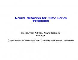
Fig. 1: Product-based Neural Network Architecture.

A. Product-based Neural Network The architecture of the PNN model is illustrated in Figure 1. From a top-down perspective, the output of PNN is a real number yˆ ∈ (0, 1) as the predicted CTR: yˆ = σ(W3 l2 + b3 ),

(1)

where W3 ∈ R1×D2 and b3 ∈ R are the parameters of the output layer, l2 ∈ RD2 is the output of the second hidden layer, and σ(x) is the sigmoid activation function: σ(x) = 1/(1 + e−x ). And we use Di to represent the dimension of the i-th hidden layer. The output l2 of the second hidden layer is constructed as l2 = relu(W2 l1 + b2 ),

(2)

D1

where l1 ∈ R is the output of the first hidden layer. The rectified linear unit (relu), defined as relu(x) = max(0, x), is chosen as the activation function for hidden layer output since it has outstanding performance and efficient computation. The first hidden layer is fully connected with the product layer. The inputs to it consist of linear signals lz and quadratic signals lp . With respect to lz and lp inputs, separately, the formulation of l1 is: l1 = relu(lz + lp + b1 ),

(3)

where all lz , lp and the bias vector b1 ∈ RD1 . Then, let us define the operation of tensor inner product: X A B , Ai,j Bi,j , (4) i,j

where firstly element-wise multiplication is applied to A, B, then the multiplication result is summed up to a scalar. After that, lz and lp are calculated through z and p, respectively:
lzn = Wzn z (5) lz = lz1 , lz2 , . . . , lzn , . . . , lzD1 ,
lp = lp1 , lp2 , . . . , lpn , . . . , lpD1 , lpn = Wpn p where Wzn and Wpn are the weights in the product layer, and their shapes are determined by z and p respectively.

By introducing a “1” constant signal, the product layer can not only generate the quadratic signals p, but also maintaining the linear signals z, as illustrated in Figure 1. More specifically,

z = z1 , z2 , . . . , zN , f1 , f2 , . . . , fN , (6) p = {pi,j }, i = 1...N, j = 1...N,

(7)

M

where fi ∈ R is the embedding vector for field i. pi,j = g(fi , fj ) defines the pairwise feature interaction. Our PNN model can have different implementations by designing different operation for g. In this paper, we propose two variants of PNN, namely IPNN and OPNN, as will be discussed later. The embedding vector fi of field i, is the output of the embedding layer: fi = W0i x[starti : endi ],

(8)

where x is the input feature vector containing multiple fields, and x[starti : endi ] represents the one-hot encoded vector for field i. W0 represents the parameters of the embedding layer, and W0i ∈ RM ×(endi −starti +1) is fully connected with field i. Finally, supervised training is applied to minimize the log loss, which is a widely used objective function capturing divergence between two probability distributions: L(y, yˆ) = −y log yˆ − (1 − y) log(1 − yˆ),

B. Inner Product-based Neural Network In this section, we demonstrate the Inner Product-based Neural Network (IPNN). In IPNN, we firstly define the pairwise feature interaction as vector inner product : g(fi , fj ) = hfi , fj i. With the constant signal “1”, the linear information z is preserved as: M N X X

(Wzn )i,j zi,j .

(10)

i=1 j=1

As for the quadratic information p, the pairwise inner product terms of g(fi , fj ) form a square matrix p ∈ RN ×N . Recalling the definition of lp in Eq. (5), lpn = PN PN n j=1 (Wp )i,j pi,j and the commutative law in vector i=1 inner product, p and Wpn should be symmetric. Such pairwise connection expands the capacity of the neural network, but also enormously increases the complexity. In this case, the formulation of l1 , described in Eq. (3), has the space complexity of O(D1 N (M + N )), and the time complexity of O(N 2 (D1 + M )), where D1 and M are the hyper-parameters about network architecture, N is the number of input fields. Inspired by FM [20], we come up with the idea of matrix factorization to reduce complexity. By introducing the assumption that Wpn = θ n θ n T , where n θ ∈ RN , we can simplify l1 ’s formulation as: Wpn p =

N X N X i=1 j=1

N N X X θin θjn hfi , fj i = h δin , δin i i=1

i=1

  X X X lp = k δi1 k, . . . , k δin k, . . . , k δiD1 k . i

(11)

i

(12)

i

By reduction of lp in Eq. (12), the space complexity of l1 becomes O(D1 M N ), and the time complexity is also O(D1 M N ). In general, l1 complexity is reduced from quadratic to linear with respect to N . This well-formed equation makes reusable for some intermediate results. Moreover, matrix operations are easily accelerated in practice with GPUs. More generally, we discuss K-order decomposition of Wpn at the end of this section. We should point out that Wpn = θn θnT is only the first order decomposition with a strong assumption. The general matrix decomposition method can be derived that: Wpn p =

N N X X hθni , θnj ihfi , fj i.

(13)

i=1 j=1

(9)

where y is the ground truth (1 for click, 0 for non-click), and yˆ is the predicted CTR of our model as in Eq. (1).

lzn = Wzn z =

where, for convenience, we use δin ∈ RM to denote a feature vector fi weighted by θin , i.e.
δin = θin fi . And we also have n δ n = δ1n , δ2n , . . . , δin , . . . , δN ∈ RN ×M . With the first order decomposition on n-th single node, we give the lp complete form:

In this case, θni ∈ RK . This general decomposition is more expressive with weaker assumptions, but also leading to K times model complexity. C. Outer Product-based Neural Network Vector inner product takes a pair of vectors as input and outputs a scalar. Different from that, vector outer product takes a pair of vectors and produces a matrix. IPNN defines feature interaction by vector inner product, while in this section, we discuss the Outer Product-based Neural Network (OPNN). The only difference between IPNN and OPNN is the quadratic term p. In OPNN, we define feature interaction as g(fi , fj ) = fi fjT . Thus for every element in p, pi,j ∈ RM ×M is a square matrix. For calculating l1 , the space complexity is O(D1 M 2 N 2 ) , and the time complexity is also O(D1 M 2 N 2 ). Recall that D1 and M are the hyper-parameters of the network architecture, and N is the number of the input fields, this implementation is expensive in practice. To reduce the complexity, we propose the idea of superposition. By element-wise superposition, we can reduce the complexity by a large step. Specifically, we re-define p formulation as p=

N X N X i=1 j=1

fi fjT = fΣ (fΣ )T ,

fΣ =

N X

fi ,

(14)

i=1

where p ∈ RM ×M becomes symmetric, thus Wpn should also be symmetric. Recall Eq. (5) that Wp ∈ RD1 ×M ×M . In this case, the space complexity of l1 becomes O(D1 M (M + N )), and the time complexity is also O(D1 M (M + N )).

D. Discussions

B. Model Comparison

Compared with FNN [12], PNN has a product layer. If removing lp part of the product layer, PNN is identical to FNN. With the inner product operator, PNN is quite similar with FM [20]: if there is no hidden layer and the output layer is simply summing up with uniform weight, PNN is identical to FM. Inspired by Net2Net [21], we can firstly train a part of PNN (e.g., the FNN or FM part) as the initialization, and then start to let the back propagation go over the whole net. The resulted PNN should at least be as good as FNN or FM. In general, PNN uses product layers to explore feature interactions. Vector products can be viewed as a series of addition/multiplication operations. Inner product and outer product are just two implementations. In fact, we can define more general or complicated product layers, gaining PNN better capability in exploration of feature interactions. Analogous to electronic circuit, addition acts like “OR” gate while multiplication acting like “AND” gate, and the product layer seems to learn rules other than features. Reviewing the scenario of computer vision, while pixels in images are real-world raw features, categorical data in web applications are artificial features with high levels and rich meanings. Logic is a powerful tool in dealing with concepts, domains and relationships. Thus we believe that introducing product operations in neural networks will improve networks’ ability for modeling multi-field categorical data.

We compare 7 models in our experiments, which are implemented with TensorFlow4 , and trained with Stochastic Gradient Descent (SGD). LR: LR is the most widely used linear model in industrial applications [22]. It is easy to implement and fast to train, however, unable to capture non-linear information. FM: FM has many successful applications in recommender systems and user response prediction tasks [20]. FM explores feature interactions, which is effective on sparse data. FNN: FNN is proposed in [12], being able to capture highorder latent patterns of multi-field categorical data. CCPM: CCPM is a convolutional model for click prediction [13]. This model learns local-global features efficiently. However, CCPM highly relies on feature alignment, and is lack of interpretation. IPNN: PNN with inner product layer III-B. OPNN: PNN with outer product layer III-C. PNN*: This model has a product layer, which is a concatenation of inner product and outer product. Additionally, in order to prevent over-fitting, the popular L2 regularization term is added to the loss function L(y, yˆ) when training LR and FM. And we also employ dropout as a regularization method to prevent over-fitting when training neural networks.

IV. E XPERIMENTS In this section, we present our experiments in detail, including datasets, data processing, experimental setup, model comparison, and the corresponding analysis1 . In our experiments, PNN models outperform major state-of-the-art models in the CTR estimation task on two real-world datasets. A. Datasets 1) Criteo: Criteo 1TB click log2 is a famous ad tech industry benchmarking dataset. We select 7 consecutive days of samples for training, and the next 1 day for evaluation. Because of the enormous data volume and high bias, we apply negative down-sampling on this dataset. Define the down-sampling ratio as w, the predicted CTR as p, the recalibrated CTR q should be q = p/(p + 1−p w ) [4]. After down-sampling and feature mapping, we get a dataset, which comprises 79.38M instances with 1.64M feature dimensions. 2) iPinYou: The iPinYou dataset3 is another real-world dataset for ad click logs over 10 days. After one-hot encoding, we get a dataset containing 19.50M instances with 937.67K input dimensions. We keep the original train/test splitting scheme, where for each advertiser the last 3-day data are used as the test dataset while the rest as the training dataset. 1 We release the repeatable experiment code on GitHub: https://github.com/ Atomu2014/product-nets 2 Criteo terabyte dataset download link: http://labs.criteo.com/downloads/ download-terabyte-click-logs/. 3 iPinYou dataset download link: http://data.computational-advertising.org. We only use the data from season 2 and 3 because of the same data schema.

C. Evaluation Metrics Four evaluation metrics are tested in our experiments. The two major metrics are: AUC: Area under ROC curve is a widely used metric in evaluating classification problems. Besides, some work validates AUC as a good measurement in CTR estimation [15]. RIG: Relative Information Gain, RIG = 1 − N E, where NE is the Normalized Cross Entropy [4]. Besides, we also employ Log Loss (Eq. (9)) and root mean square error (RMSE) as our additional evaluation metrics. D. Performance Comparison Table I and II show the overall performance on Criteo and iPinYou datasets, respectively. In FM, we employ 10order factorization and correspondingly, we employ 10-order embedding in network models. CCPM has 1 embedding layer, 2 convolution layers (with max pooling) and 1 hidden layer (5 layers in total). FNN has 1 embedding layer and 3 hidden layers (4 layers in total). Every PNN has 1 embedding layer, 1 product layer and 3 hidden layers (5 layers in total). The impact of network depth will be discussed later. The LR and FM models are trained with L2 norm regularization, while FNN, CCPM and PNNs are trained with dropout. By default, we set dropout rate at 0.5 on network hidden layers, which is proved effective in Figure 2. Further discussions about the network architecture will be provided in Section IV-E. 4 TensorFlow:

https://www.tensorflow.org/

TABLE I: Overall Performance on the Criteo Dataset. AUC 71.48% 72.20% 75.66% 76.71% 77.79% 77.54% 77.00%

Log Loss 0.1334 0.1324 0.1283 0.1269 0.1252 0.1257 0.1270

RMSE 9.362e-4 9.284e-4 9.030e-4 8.938e-4 8.803e-4 8.846e-4 8.988e-4

RIG 6.680e-2 7.436e-2 1.024e-1 1.124e-1 1.243e-1 1.211e-1 1.118e-1

TABLE II: Overall Performance on the iPinYou Dataset. Model LR FM FNN CCPM IPNN OPNN PNN*

AUC 73.43% 75.52% 76.19% 76.38% 79.14% 81.74% 76.61%

Log Loss 5.581e-3 5.504e-3 5.443e-3 5.522e-3 5.195e-3 5.211e-3 4.975e-3

RMSE 5.350e-07 5.343e-07 5.285e-07 5.343e-07 4.851e-07 5.293e-07 4.819e-07

RIG 7.353e-2 8.635e-2 9.635e-2 8.335e-2 1.376e-1 1.349e-1 1.740e-1

TABLE III: P-values under the Log Loss Metric. Model IPNN OPNN

LR < 10−6 < 10−6

FM < 10−6 < 10−5

FNN < 10−6 < 10−6

CCPM < 10−6 < 10−6

80.0%

AUC on iPinYou

Model LR FM FNN CCPM IPNN OPNN PNN*

85.0%

75.0%

LR FM FNN CCPM IPNN OPNN

70.0%

65.0%

60.0%

2

4

6

8

10

Iterations

12

14

16

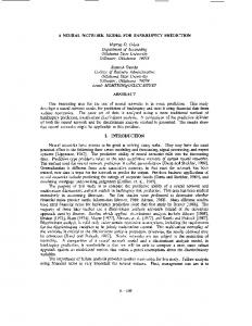
Fig. 3: Learning Curves on the iPinYou Dataset.

models converge more quickly than LR and FM. We also observe that our two proposed PNNs have better convergence than other network models. E. Ablation Study on Network Architecture

78.0%

Criteo AUC

77.5% 77.0% 76.5% 76.0% 75.5% 75.0%

0.1

0.2

0.3

0.4

0.5

0.6

Dropout

0.7

0.8

0.9

Fig. 2: AUC Comparison of Dropout (OPNN).

Firstly, we focus on the AUC performance. The overall results in Table I and II illustrate that (i) FM outperforms LR, demonstrating the effectiveness of feature interactions; (ii) Neural networks outperform LR and FM, which validates the importance of high-order latent patterns; (iii) PNNs perform the best on both Criteo and iPinYou datasets. As for log loss, RMSE and RIG, the results are similar. We also conduct t-test between our proposed PNNs and the other compared models. Table III shows the calculated p-values under log loss metric on both datasets. The results verify that our models significantly improve the performance of user response prediction against the baseline models. We also find that PNN*, which is the combination of IPNN and OPNN, has no obvious advantages over IPNN and OPNN on AUC performance. We consider that IPNN and OPNN are sufficient to capture the feature interactions in multi-field categorical data. Figure 3 shows the AUC performance with respect to the training iterations on iPinYou dataset. We find that network

In this section, we discuss the impact of neural network architecture. For IPNN and OPNN, we take three hyperparameters (or settings) into consideration: (i) embedding layer size, (ii) network depth and (iii) activation function. Since CCPM shares few similarities with other neural networks and PNN* is just a combination of IPNN and OPNN, we only compare FNN, IPNN and OPNN in this section. 1) Embedding Layer: The embedding layer is to convert sparse binary inputs to dense real-value vectors. Take word embedding as an example [11], an embedding vector contains the information of the word and its context, and indicates the relationships between words. We take the idea of embedding layer from [12]. In this paper, the latent vectors learned by FM are explained as node representations, and the authors use a pre-trained FM to initialize the embedding layers in FNN. Thus the factorization order of FM keeps consistent with the embedding order. The input units are fully connected with the embedding layer within each field. We compare different orders, like 2, 10, 50 and 100. However, when the order grows larger, it is harder to fit the parameters in memory, and the models are much easier to over-fit. In our experiments, we take 10-order embedding in neural networks. 2) Network Depth: We also explore the impact of network depth by adjusting the number of hidden layers in FNN and PNNs. We compare different number of hidden layers: 1, 3, 5 and 7. Figure 4 shows the performance as network depth grows. Generally speaking, the networks with 3 hidden layers have better generalization on the test set. For convenience, we call convolution layers and product layers as representation layers. These layers can capture complex feature patterns using fewer parameters, thus are efficient in training, and generalize better on the test set.

78.5%

FNN IPNN OPNN

77.5%

FNN IPNN OPNN

0.13 0.12

77.0%

RIG

AUC Performance

78.0%

76.5% 76.0% 75.5%

0.11 0.10

75.0% 74.5%

1

2

3

4

5

Hidden Layers

6

0.09

7

1

2

3

4

5

Hidden Layers

6

7

Fig. 4: Performance Comparison over Network Depths. 78.0%

80%

76.5% 76.0% 75.5%

79% 78% 77%

75.0%

76%

74.5%

75%

74.0%

FNN

IPNN

Models

sigmoid tanh relu

81%

iPinYou AUC

77.0%

Criteo AUC

82%

sigmoid tanh relu

77.5%

OPNN

74%

FNN

IPNN

Models

OPNN

Fig. 5: AUC Comparison over Various Activation Functions.

3) Activation Function: We compare three mainstream ac−2x tivation functions: sigmoid(x) = 1+e1−x , tanh(x) = 1−e 1+e−2x , and relu(x) = max(0, x). Compared with the sigmoidal family, relu function has the advantages of sparsity and efficient gradient, which is possible to gain more benefits on multi-field categorical data. Figure 5 compares these activation functions on FNN, IPNN and OPNN. From this figure, we find that tanh has better performance than sigmoid. This is supported by [12]. Besides tanh, we find relu function also has good performance. Possible reasons include: (i) Sparse activation, nodes with negative outputs will not be activated; (ii) Efficient gradient propagation, no vanishing gradient problem or exploding effect; (iii) Efficient computation, only comparison, addition and multiplication. V. C ONCLUSION AND F UTURE W ORK In this paper, we proposed a deep neural network model with novel architecture, namely Product-based Neural Network, to improve the prediction performance of DNN working on categorical data. And we chose CTR estimation as our working example. By exploration of feature interactions, PNN is promising to learn high-order latent patterns on multi-field categorical data. We designed two types of PNN: IPNN based on inner product and OPNN based on outer product. We also discussed solutions to reduce complexity, making PNN efficient and scalable. Our experimental results demonstrated that PNN outperformed the other state-of-the-art models in 4 metrics on 2 datasets. To sum up, we obtain the following

conclusions: (i) By investigating feature interactions, PNN gains better capacity on multi-field categorical data. (ii) Being both efficient and effective, PNN outperforms major stateof-the-art models. (iii) Analogous to “AND”/“OR” gates, the product/add operations in PNN provide a potential strategy for data representation, more specifically, rule representation. In the future work, we will explore PNN with more general and complicated product layers. Besides, we are interested in explaining and visualizing the feature vectors learned by our models. We will investigate their properties, and further apply these node representations to other tasks. R EFERENCES [1] A. K. Menon, K.-P. Chitrapura, S. Garg et al., “Response prediction using collaborative filtering with hierarchies and side-information,” in SIGKDD. ACM, 2011, pp. 141–149. [2] G.-R. Xue, H.-J. Zeng, Z. Chen, Y. Yu, W.-Y. Ma, W. Xi, and W. Fan, “Optimizing web search using web click-through data,” in CIKM, 2004. [3] W. Zhang, S. Yuan, and J. Wang, “Optimal real-time bidding for display advertising,” in SIGKDD. ACM, 2014, pp. 1077–1086. [4] X. He, J. Pan, O. Jin et al., “Practical lessons from predicting clicks on ads at facebook,” in Proceedings of the Eighth International Workshop on Data Mining for Online Advertising. ACM, 2014, pp. 1–9. [5] K.-c. Lee, B. Orten, A. Dasdan et al., “Estimating conversion rate in display advertising from past erformance data,” in SIGKDD. ACM, 2012, pp. 768–776. [6] A.-P. Ta, “Factorization machines with follow-the-regularized-leader for ctr prediction in display advertising,” in IEEE BigData. IEEE, 2015, pp. 2889–2891. [7] Y. Cui, R. Zhang, W. Li et al., “Bid landscape forecasting in online ad exchange marketplace,” in SIGKDD. ACM, 2011, pp. 265–273. [8] Y. LeCun, Y. Bengio, and G. Hinton, “Deep learning,” Nature, 2015. [9] A. Krizhevsky, I. Sutskever, and G. E. Hinton, “Imagenet classification with deep convolutional neural networks,” in NIPS, 2012, pp. 1097– 1105. [10] A. Graves, A.-r. Mohamed, and G. Hinton, “Speech recognition with deep recurrent neural networks,” in ICASSP. IEEE, 2013, pp. 6645– 6649. [11] T. Mikolov, I. Sutskever, K. Chen et al., “Distributed representations of words and phrases and their compositionality,” in NIPS, 2013, pp. 3111–3119. [12] W. Zhang, T. Du, and J. Wang, “Deep learning over multi-field categorical data: A case study on user response prediction,” ECIR, 2016. [13] Q. Liu, F. Yu, S. Wu et al., “A convolutional click prediction model,” in CIKM. ACM, 2015, pp. 1743–1746. [14] M. Richardson, E. Dominowska, and R. Ragno, “Predicting clicks: estimating the click-through rate for new ads,” in WWW. ACM, 2007, pp. 521–530. [15] T. Graepel, J. Q. Candela, T. Borchert et al., “Web-scale bayesian clickthrough rate prediction for sponsored search advertising in microsoft’s bing search engine,” in ICML, 2010, pp. 13–20. [16] K. Ren, W. Zhang, Y. Rong, H. Zhang, Y. Yu, and J. Wang, “User response learning for directly optimizing campaign performance in display advertising,” in CIKM, 2016. [17] Y. Zhang, H. Dai, C. Xu et al., “Sequential click prediction for sponsored search with recurrent neural networks,” arXiv preprint arXiv:1404.5772, 2014. [18] A. P. Engelbrecht, A. Engelbrecht, and A. Ismail, “Training product unit neural networks,” 1999. [19] W. Zhang, S. Yuan, and J. Wang, “Real-time bidding benchmarking with ipinyou dataset,” arXiv:1407.7073, 2014. [20] S. Rendle, “Factorization machines,” in ICDM. IEEE, 2010, pp. 995– 1000. [21] T. Chen, I. Goodfellow, and J. Shlens, “Net2net: Accelerating learning via knowledge transfer,” in ICLR, 2016. [22] H. B. McMahan, G. Holt, D. Sculley et al., “Ad click prediction: a view from the trenches,” in SIGKDD. ACM, 2013, pp. 1222–1230.