Multimedia Tools and Applications, 1, 9-46 (1995) Q 1995 Kluwer Academic Publishers, Boston. Manufactured in The Netherlands.
Production Model Based Digital Video Segmentation ARUN HAMPAPUR, RAMESH JAIN* AND TERRY E W E Y M O U T H
[email protected] Computer Science and Engineering, Department of Electrical Engineering and Computer Science,University of Michigan, 1101 Beal Ave, Ann Arbor, MI 48109-2110
Abstract. Effective and efficient tools for segmenting and content-basedindexing of digital video are essential to allow easy access to video-based information. Most existing segmentation techniques do not use explicit models of video. The approach proposed here is inspired and influenced by well established video production processes. Computational models of these processes are developed. The video models are used to classify the transition effects used in video and to design automatic edit effect detection algorithms. Video segmentation has been formulated as a production model based classification problem. The video models are also used to define segmentation error measures. Experimental results from applying the proposed technique to commercial cable television programming are presented. Keywords: Digital Video, Video Segmentation, Video Indexing, Video Databases, Edit Effects, Fade In, Fade Out, Dissolve, Editing, Content based retrieval
1.
Introduction
The progress of computer systems towards becoming true multimedia machines depends largely on the set of tools available for manipulating the different components of multimedia. Of these components digital video is the most data intensive. Effective tools for segmenting and content based indexing of digital video are essential in the design of the true multimedia machine. This paper presents an innovative and novel approach to modeling and segmenting digital video based on video production techniques. The problem of segmenting digital video occurs in many different application of video. Content based access of video in the context of video databases requires access to video in a more natural unit than frames. Video segments based on edit locations provides a higher level of access to video than frames. Multimedia authoring systems which reuse produced video need access to video in terms of video shots. The edit detection algorithms presented in this paper can be used in digital video editing systems for edit logging operations. There are several other applications in video archiving and movie production which can use the segmentation techniques presented here. Video segmentation requires the use of explicit models of video. Most o f the current approaches to video segmentation [1], [19], [24], [22] do not use explicit models. They pose the problem as one of detecting camera motion breaks in arbitrary image sequences. The solutions that have been presented typically involve the application of various low level image processing operations to the video sequences. These approaches have not utilized the inherent structure o f video. Defining models o f video which capture the * Currently at the University of California, San Diego, La Jolla, CA 92093-0407
10
ARUN HAMPAPUR, RAMESH JAIN AND TERRY E. WEYMOUTH
structure provides the constraints necessary for effective video segmentation. Hampapur et al [10] have presented initial results on model based video segmentation. The work presented in this paper uses the production model based classification approach to video segmentation. This paper presents a video edit model which is based on a study of video production processes. This model captures the essential aspects of video editing. Video features extractors for measuring image sequence properties are designed based on the video edit model. The extracted features are used in a production model based classification formulation to segment the video. The models are also used to define error measures, which in conjunction with test videos and correct video models are used to evaluate the performance of the segmentation system. Experimental results from segmenting commercial cable television data are presented. Section 2 discusses modeling of digital video based on video production techniques and proposes a classification of edits. Video segmentation is defined in section 3. The formulation of video segmentation as production model based classification is discussed in section 4. This section also presents the design of feature extractors. The classification and segmentation steps are discussed in 5. Section 6 presents a comparison of this work to other research in the field. Segmentation error measures are formulated in section 7. Section 8 presents the experiments performed and the results obtained. A summary of the work and future directions concludes the paper.
2. Modeling Digital Video Video (the term video is used generically to cover movies, video, cable television programming etc) is a means of storing and communicating information. There are many different ways in which video is used and many different aspects of video [8], [14]. The two most essential aspects of video are the content and the production style. The content of video is the information that is being transmitted through the medium of video. The production style is the encoding of the content into the medium of video. The production style of video is the aspect which is directly relevant to the problem of segmenting digital video. The process of producing a video involves two major steps, the production of shots (a sequence of frames generated by a single operation of the camera [17]), shooting and the compilation of the different shots into a structured audio visual presentation, editing [17], [2]. In order to segment video it is essential to have a computational model of the editing process. Figures 1, 2 illustrates the process of editing. The two phases are as follows: Editing This is the process of deciding the temporal ordering of shots. It also involves deciding on the transitions or edits to be used between different shots. The result of the editing process is a list or a model called the Edit Decision List[6]. Assembly This is the physical process which the Edit Decision List is converted into frames on the final cut [2]. This is the process involves taking the shots from the
PRODUCTION MODEL BASED DIGITAL VIDEO SEGMENTATION
11
f Video Production Model
J Figure 1. Video Production Model
shot set in the specified order, and implementing the edits between the shots. The assembly process in general adds frames called edit frames to the final cut in addition to the frames from the original shots.
2.1.
Video Edit Model
The video edit model presented here captures the process of editing and assembly discussed in the previous section. The model has three components, the Edit Decision Model which models the output of the editing, the Assembly Model which represents the assembling phase of video production and the Edit Effect Model which describes the exact nature of the image sequence transformation that occurs during the different types of edit effects. Consider a set of shots S = ($1, $2, ....SN) with cardinality N. Each shot Si c S can be represented by a closed time interval:
Si = [tb,/;e]
(1)
where tb is the time at which the shot begins and te is the time at which the shot ends. Before the final cut is made tb = 0 '~' Si C S since there is no relative ordering of the shots. Let E = (El, E2, ...Ek) be the set edits available. Each edit E is represented by a triple:
12
ARUN HAMPAPUR, RAMESH JAIN AND TERRY E. WEYMOUTH
fVideo Production Model: AssemblingOperation~ Shot 1 Final Cut
Shot 1
/-T--
1 Shot1 begin
,~hot2
Edit
Shot2
Shot,!1ndSho'!n' B~176 Beg,,., Edit End
Edit Decision List
J
Figure 2. Video Production Model: Assembly Operation
E = {[tb, tel, T, e}
(2)
where [tb, t~] is the duration of the edit, T e (T1, ~'2, ..T,~) is the type of the edit (typical examples include cuts, fades, dissolves) and e is the the mathematical transformation that is applied during an edit or the edit effect model. Consider a video V. Let V be composed of n shots taken from the set S. Then the Edit Decision Model V~dm can be represented as follows. Yedm =
$1 o E12($1, $2) o $2 o E23(~'2, $3) o .
.
.
o s(~_1) o
E(~_I)~(S~-I, S~)
o S,~
(3)
where S i c S, the subscript i denotes the temporal position of the shot in the sequence (i.e. if i < j shot Si appears before shot Sj in the final cut ) and Eij denotes the edit transition between shots S{ and Sj. The o denotes the concatenation operation and E~j C E. The Assembly Model for V is given by: Y a m = $1 o S e l 2 0 S 2 o Se23 o . . .
o S(n_l) o Se(n_l) n o S n
(4)
where Sx represent the shots used to compose the video and S ~ x represent the edit
frames. The assembly model can be rewritten as follows: Y c = 81 o 82 o s 3 o 8 4 o . . .
o 8(n_1) o s n o S(n+l ) o8(2n_1)
si = {its, t~], I d
li e (edit, shot)
(5)
PRODUCTION MODEL BASED DIGITAL VIDEO SEGMENTATION
13
Table I. Edit Types Type Name
T~
Tc
Meaning
Duration Examples
1
Identity
T
I
ConcatenateShots
Zero
Cut
2
Spatial
Ts
I
Manipulateshot pixel space
Finite
Translate,Page
3
Chromatic f
Te
Manipulateshot intensity space
Finite
Fade, Dissolve
4
Combined Ts
Tc
Manipulatepixels and intensities Finite
Morphing
V~ is called the video computational model. In this representation, every segment of video is a temporal interval with a label indicating the content. Segmentation of video requires two labels namely,(shot, edit). It is important to keep in mind that the edit frames are also image sequences, they differ from shots in the production technique used. Cuts are a special type of interval with zero length. This computational model of video is used to define error measurements in the later sections.
2.2.
Edit Effect Model
The edit effects commonly used in video production are modeled by using 2D image transformations [23]. The mathematical model for the process of generating edit frames from a pair of shots is discussed in this section. Consider an image sequence, where the pixel positions are denoted by x, y and the frame number is denoted by t. Let r, g, b denote the three (red,zgreen,blue) color values assigned to each pixel. Let the image space be denoted by ~ = {x, y, t, 1} and the color space be denoted by ~ = {r, g, b, 1}. Homogeneous Coordinates [5] are used for representing both the image and color spaces in order to accommodate affine transformations. Using these notations and assuming linear affine transformations, the possible set of edit frames E(x, !I, t) given two shots So~t (x, y, t) and S ~ ( x, y, t) can be denoted as follows.
E ( x , y , t ) = So~t((x T8I) x Tcl | Sin((X Ts2 ) x Tc2
(6)
Here Sout represents the shot before the edit or the out going shot and S~,~ represents the shot after the edit or the incoming shot, Ts and Tc denote the transformation applied to the pixel and color space of the shots being edited and | denotes the function used to combine the two shots in order to generate the set of edit frames. In general T8 and Tc can be any type of transformation (linear, non-linear) and @ can be any operation. In practice however, the transformations are either linear or piecewise linear and the operation | is addition. The remainder of the discussion assumes this simplified edit effect model. Edit effects are classified into four types based on the nature of the transformation used during the editing process. Table 1 shows a classification of edit effects, f denotes the identity transformation.
14
ARUN HAMPAPUR, RAMESH JAIN AND TERRY E. WEYMOUTH
The classification presented in table 1 has a simple physical explanation. The classes correspond to the different types of operations that an editor can perform when editing two shots. The options are: Type 1: Identity Class: Here the editing process does not modify either of the shots. No additional edit frames are added to the final cut. Cuts comprise this class of edits.
Type 2: Spatial Class: Only the spatial aspect of the two shots is manipulated by this class of edit effects. The color space of the shots is not affected. This class is comprised of effects like page translates, page turns, shattering edits and many other digital video effects. Type 3: Chromatic Class: Edits in this class include fade in's, fade out's and dissolves. Here the edit effect manipulates the color space of either of the shots without changing the spatial relation of any of the pixels.
Type 4: Spatio-Chromatic Class: Here both the space and color aspects of the shots is simultaneously manipulated during the editing process. This class consists of effects like image morphing and wipes.
3. Video Segmentation: Problem Definition Video segmentation is the process of decomposing a video into its component units. There are two equivalent definitions of video segmentation: Shot Boundary Detection: Given a video V (equation 3) composed from n shots, V Si E V locate
[~b, re]the extremal points
of the shot
(7)
Edit Boundary Detection: Given a video V (equation 3) composed from n shots, ~/Ei E V locate [tb, re]the extremal points of the edit
(8)
The above two definitions are equivalent as edits and shots form a partition of the video. These two definitions are analogous to the the region growing vs edge detection approaches to image segmentation [20]. The techniques proposed in this paper treat video segmentation as edit boundary detection. The reasons for this choice is the relative simplicity of edit effect models as compared to shot models. Edits are simple effects that are artificially introduced using an editing suite to compose a video [2]. Shots on the other hand incorporate all the factors that affect the static image formation process and the changes of these factors over time. This makes shots much harder to model analytically as compared to edits [8], [9].
PRODUCTION MODEL BASED DIGITAL VIDEO SEGMENTATION
4.
15
Video segmentation using production model based classification
Video segmentation is formulated as a production model based classification problem. In production model based classification the essential aspect is the existence of a computational model of the data production process. This data production model is used in designing feature extractors which are used in the automatic analysis of the data which is being classified. The use of the data production model distinguishes production model based classification from the traditional feature based classification [3]. The video edit model (equation 3,4,5) and the edit effect models (equation 6) are the data production models in video segmentation.
f
Production Model based Digital Video Segmentation
~'~
tionModel dit M~
Video
[ Feature
J
L f
Fvide~ s
f
V
I
~J
Figure 3. ProductionModelbased VideoSegmentation: BlockDiagram Figure 3 shows the stages in model based classification. The design phase of the problem has the following steps:
Production Model Formulation: This step involves the study of the data production process (in this case video and film editing) to develop a model of the process. The first step is to isolate the essential steps used in data production. These steps are then translated into computational models. Feature Extractor Design: Here the production models developed in the previous step are used to systematically design features extractors which can be applied to the data in the automatic analysis phase.
16
ARUN HAMPAPUR, RAMESH JAIN AND TERRY E. WEYMOUTH
The analysis or online portion of the production model based classification approach is the feature based classification process [3] where the feature extractors previous designed are used. The steps in feature based classification are:
Feature Extraction: The data to be classified is processed by the feature extractors to generate features which are indicators of the data classes of interest. Classification: The different features extracted in the previous step are combined using a discriminant function to assign a class label to the data set being classified. In the current formulation of video segmentation as production model based classification, the four edit classes (table 1) are the classes of interest. Feature extractors are designed for each of these classes (in this work only the first three classes are used). The feature extractors are applied to the individual frames of the video. The features are combined using a discriminant function to assign to each frame of video the label edit or shot. The segmentation block essentially groups the frames into segments based on the labels assigned. A finite state machine is used to achieve this segmentation step. The following subsections present the different steps of the formulation. Section 4.1 presents the details of the identity edit class. The various details of the chromatic edit class are discussed in section 4.2. The spatial edit class is presented in section 4.4. The computational requirements of the feature detectors and a summary are presented in sections 4.6, 4.7. Section 5 discusses the classification and segmentation process.
4.1.
Cut Detection
A cut is an identity edit and unlike other edits cannot be modeled or defined independently of the two shots it concatenates, since it does not contribute any edit frames to the video. Cuts can be categorized in terms of the shots that they concatenate. When a video with a cut is presented to a viewer, the viewer will experience a sudden transition (or discontinuity) of visual properties across the transition. Visual properties of a shot include factors like speed and direction of motion of objects and camera, shapes, color, brightness distribution, etc. During the editing phase of video production, the director controls various visual property transitions across a cut. Some directors try to minimize the visual discontinuity experienced by the viewers across a cut. This criterion is termed as a graphic match[2], [7] in editing literature, others maximize the visual discontinuity across the cut to evoke a specific viewer reaction. A cut detector is an algorithm which can detect the discontinuity of a certain visual property across two consecutive frames in a video. Most of the cut detectors used in literature [1], [19], [24], [22] rely on the color space of the frames to identify a discontinuity. The techniques also have an implicit shot model in terms of the expected variation of the visual property within the bounds of the shot. The performance of these detectors is fairly acceptable and accuracies in the range of 90% to 95% have been reported. There are two ways of achieving better cut detection, use additional visual properties and use explicit models of shots. There are several techniques [21] which can be used to identify discontinuity of feature tracks in image sequences and
PRODUCTION MODEL BASED DIGITAL VIDEO SEGMENTATION
17
Table 2. Cut features
Name
Measurement Formula
Description
Template Matching
)-'~z,y IS(x, y, t) - S(x, y, t + 1)1
IntensityDifference
Histogram X2
G (Ht(i)--H~+l(i)) 2 ~-~i=o H t + a (i)
X z IntensityDistribution comparison
other such properties. The problem of developing general models of video shots is an extremely difficult problem due to the number of factors that affect the nature of the video data. However different aspect of video can be individually modeled and used in developing tuned cut detectors. Work on modeling video for the purpose of video analysis is presented in [8]. Cut detectors used in this work are based on results presented by other researchers [1], [19], [24], [22] in the field. The operators presented by Nagasaka et al and Smoliar et al were used in an extensive experimental study using cable TV data. Table 2 shows two features for cut deiection that have been proposed in literature. Consider a shot S. Let the pixel size of the frames be N~ • Ny. Let G be the number of gray levels. Let t denote the time or the frame number. Let the shot length be L. Let x, y denote pixel location within a frame. Let H~ be the histogram of the t th frame of the shot. These features were extracted from videos with cuts between different types of shots (object motion shots, camera motion shots, etc). The two features shown in table 2 were used in the development of the segmentation system presented in this work.
4.2.
C h r o m a t i c E d i t Detector
Chromatic editing manipulates the color space of the two shots being edited (table I). The goal of the chromatic edit detector is to discriminate between intensity changes due to chromatic editing as opposed to intensity changes due to scene activity. The intensity changes in the image sequence resulting from chromatic editing have a particular pattern which is modeled analytically by the edit effect model. The chromatic edit detector analyses the video data and detects the presence of the data patterns conforming to the edit effect model. Fades and Dissolves are the two most prevalent types of chromatic edits. These edit effects are used as the focus of the rest of the discussion.
4.2.1.
Chromatic Scaling
Fades and dissolves can be modeled as chromatic scaling operations. During a fade one of the shots being edited is a constant (normally black). A dissolve typically involves the scaling of two shots that are being edited. Thus a detector which can detect chromatic scaling in a video can be used to detect both fades and dissolves. The following discussion presents the model for a chromatic scaling of an image sequence, and derives a feature
18
ARUN HAMPAPUR, RAMESH JAIN AND TERRY E. WEYMOUTH
for detecting such an effect in a video. Once the scaling detector is designed, the use of that detector for detecting fades and dissolves is discussed. Consider a gray scale sequence g(x, y, t). Let the color space of the sequence be scaled out to black over the length of ls frames. Then the model E(x, y, t) for the output video of the scaling operation is:
E(x,y,t) = g(x,y,t) x ( 1 - ~ )
(9)
During a single frame scaling, only the last frame of the shot is used in the scaling operation, i.e. the last frame of the shot is frozen and the intensity is scaled to zero (or the intensity is scaled from zero in the case of a fade in). Thus during a single frame scaling there is no motion within the sequence. In this case equation 9 can be written as 10 where k indicates that the k th frame of the shot is being used in the scaling.
(l~-t~ E ( x , y , t ) = g ( x , y , k ) x \ ls J Differentiating
(10)
E(t) with respect to time:
bE _ -g(x, y, k) 5t ls
(11)
Equation 11 can be rewritten as ~__E
~t k) _ c z ( t ) - g(x,y,
-1
(12)
where CZ chromatic image, is the scaled first order difference image. This image is a constant image with the constant value being proportional to the fade rate. A simple function based on the distribution of intensities can be designed to provide a measure of the constancy of an image. Let Fc~(t)be the chromatic scaling feature which is a measure of constancy of CZ (section 4.5).
Fr
= LI(CZ(t))
(13)
For multi-frame scaling, the scaling is done over a sequence of frames. Thus there is scene action in progress during the scaling edit. Here the differences in the pixel values during a scale will be due to a combination of the motion generated intensity difference and the scale generated intensity difference. The chromatic scaling feature, Fcs, is applicable if the change due to the editing dominates the change due to motion.
4.3.
Fades and Dissolves as Chromatic
Scaling
The fade and dissolve operations can be represented as scaling operations.
some combination of chromatic
19
P R O D U C T I O N MODEL BASED DIGITAL V I D E O S E G M E N T A T I O N
Fade Detection Two types of fades are commonly used in commercial video production, fade in from black and fade out to black. In both these cases the fades can be modelled as chromatic scaling operations with a positive and negative fade rate. Eyo equation 14 represents the sequence of images generated by fading out a video gl to black. 11 is the fade out rate in terms of the number of frames. 6 represents the black image sequence. Comparing equations 6 and 14, for a fade out one of the shots
Sour = gl, Sin = 0 and | = +. Similarly, Eyi (equation 15) represents the images generated by fading in a sequence g2, at the rate of 12. Here Sour = 0 and Sin = g2 The equations (14, 15) represent how the fade operation maps on to the edit effect model (equation 6). Since the operations on the individual sequences in the fade are chromatic scaling operations the chromatic scaling feature 12 can be used for detecting fades in videos.
(14)
Efi(x,y,t) = 0 + g2(x,y)
t
(15)
Dissolve Detection A dissolve is a chromatic scaling of two shots simultaneously. Let Ed be the set of edit frames generated by dissolving two shots S o u t = gl and Sin -- g2. Equation (16) models the process of dissolving two shots.
(11 -
Ed(x,y,t) = g l ( x , y ) \
ll
,] (tl,tl+gl)
+g2(x'Y) ( t ) ~
(16)
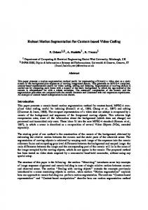
Here (tl,t2) are the times at which the scaling of gl,g2 begin and (/1,/2) are the duration for which the scaling of gl, g2 lasts. The relative values of these parameters can be used to group dissolves into different classes. Such a grouping can be used to analyze the effectiveness of the detection approach. Comparing equations (15,14) and equation 16 it can be seen that the dissolve is a combination of the fade in and fade out operation occurring simultaneously on two different shots. A dissolve is a multiple sequence chromatic scaling. Designing the dissolve detector can now be treated as a problem of verifying that the chromatic scaling detector (equation 13) can be used to detect the dissolve. The approach followed in this work is to classify the dissolves into groups based on their qualitative properties and to verify the detectability of each group using the chromatic scaling operator. Figure (4) presents the sequence activity graph (SAG) during a dissolve edit. It shows the qualitative labeling of dissolves. The hatched area indicates the Out Shot activity and the filled area the In Shot. A positive slope in the SAG indicates a fade
20
ARUN HAMPAPUR, RAMESH JAIN AND TERRY E. WEYMOUTH
in operation and the negative slope indicates a fade out operation. A zero slope in the SAG indicates no sequence activity due to editing. The basis used for the qualitative labeling is the start time and the dissolve length. The labels are based on Shot of Initial Activity-Dominating Shot attributes of the sequence, which are defined as follows: Shot of Initial Activity: This is defined as the shot s, where (tl,t2) are the times at which Out, In shots begin scaling. s = In if tl > t2 ~ Fade In begins before Fade Out s : Out if
tl < t2 ~
s = Both if tl : t2 ~
(17)
Fade Out begins before Fade In.
(18)
Fade In, Fade Out begin together.
(19)
Dominating Shot: This is defined as the shot s where (/1,/2) are the dissolve lengths of the Out, In shots respectively. s : s :
In if 11 < 12 ~ In Shot dominates dissolve
(20)
Out if 11 > 12 ~ Out Shot dominates dissolve
(21)
s = Equal if /1 = 12 ~ No Shot dominates dissolve
(22)
A shot is said to dominate the dissolve if its activity slope is higher. In other words, if the shot contributes more to the inter frame change [12], [13] in the video sequence. From figure 4 it can seen: 1. that except in the case of Both-Equal type of dissolves, all the other types have portions during which there is an exclusively single sequence chromatic scaling in progress. 2. that except in the case of Equal Dominance Sequences the change contribution of one sequence dominates the other. Thus the cases in which the chromatic scaling feature (equation 13) will not respond to the dissolve are those in which very similar sequences are being dissolved with precisely equal fade rates over the dissolve. In most commercially produced video sequences dissolves are seldom executed with such precision and dissolving very similar sequences are avoided. Hence the chromatic scaling feature can be used to detect most dissolves. The experimental studies conducted confirm these observations over a wide range of commercial video.
4.3.1.
Limitations of Chromatic Edit Detector
There are several limitations of the chromatic edit detector: Additional Chromatic Transforms: The chromatic edit detector presented can be used for detecting chromatic edits which are scalings of the color space. There are other
P R O D U C T I O N M O D E L B A S E D DIGITAL V I D E O S E G M E N T A T I O N
Dissolve Classification
21
Out Shot In Shot E t 1 > t2, I1 > 12, In-Out
t l > t 2 , 11 t2, 11 = 12, In-Equal ~
tl 12 , Out-Out
~
tl 12, Both-Out ~
t
1 = t2, 11 < 12, Both-In
~
t
1 = t2, il = 12, Both-Equal Time
-' rid
Figure 4. Sequence Activity Graph during a dissolve
possible types of chromatic transforms like chromatic translations, rotations etc which have not been addressed in this work. However this is not a serious practical limitation as chromatic transformations other than scaling are seldom used in practice. Multiple Sequence Scalings: The scaling detector is primarily designed to detect the scaling of single image sequences. It can be used to detect two sequence scalings as in the case of dissolves provided that the effect of sequence domination is present (section 4.3). If there are segments of video with dissolves of more than two sequences the chromatic scaling detector cannot be guaranteed to respond. Piecewise Transformations: The detectors are designed to respond to global image transforms. The detector responses become unpredictable if the chromatic transforms are applied to spatial sub windows in the sequence. Transformation Rates: This is the inverse of the duration for which a particular transformation is applied to create an edit. When the transformation rate is very high the extended edit approaches the cut or identity. In this case the change will be large enough for the cut detector to respond. In the case of extremely small transformation rates (dissolves and fades over 100's of frames), the change due to the effect between
22
ARUN HAMPAPUR, RAMESH JAIN AND TERRY E. WEYMOUTH
frames may be too small. In such cases detecting these effects based on two frames of video will not be possible and approaches involving extended set of frames will have to be adopted.
4.4.
Spatial Edit Detector
Spatial edits are achieved by transforming the pixel space of the shots being edited. These are Type 2 transforms in table 1 where Tc = I and T8 has different values depending on the exact nature of the spatial effect used. takes on different values depending on the specific type of spatial edit. One of the most commonly used edits is the page translate, where the shot preceeding the edit is translated out of the viewport uncovering the shot that follows the edit. This type of edit is used as an exemplifier of the class of spatial edits and a feature derivation is presented. Consider a video E ( x , y, t) with a translate spatial edit. In such an edit the first shot translates out, uncovering the second shot. Let E ( x , y, t) be a gray scale sequence for notational simplicity. Let gout(x, y, t), gin(x, y, t) be the gray scale models of the incoming and outgoing shots in the edit. Let c~x,c~y be the translation coefficients in the x and y directions respectively. Let N~, Ny be the number of pixels in the x and y dimensions of each frame. The translate edit can now be modeled as E(x,y,t) = go~t(x+~z.t,y+~v-t,t) i f 0 T
g *kcomp
O(Jkf)
Mean
~(/(t))
~ , ~ Nx(~,y,t)
N * kadd + kaiv
O(H)
Variance
~(I(t))
~-~x,y(I(x,y,t) - ,a(I(t))) 2
N * (kmutt + Ksub)
O(Jkf)
Area
A(B(t))
~,vB(x,v,t
N * k,~m
O(Af)
Centroid
C(B(U))
Cx = E ~ ' v x Id(x,y) A E ~ , y y ld(x,y) Cy = A
N * (2 * krnult) -t- kdi v
O(JV')
)
Chromatic ling
CZ
equation 12
A d l f f + Adl v
O(JV')
Spatial Img
$Z
equation 29
AdiM + Agrad + Adiv
O(Jkf)
Uniformity
LI(XZ, 7))
equation31
Adiy] -}- Athresh + Aarea + A v a r + Acentroid + A t h r e s h + kdi v + k a d d
0(~()
Cut
~cut
(1))2 ~ i =Go (Ht(i)-HL+I Ht+l (i)
3 * N * kadd'tG * (kad d + kdiv + kmult )
O(d~ + 6)
Chromatic
~chrom
Lt(CZ)
Auniform~ty + ACZ
O(N)
Spatial
ffrspace
LI(SZ)
Auni f orm~ty "4-ASZ
O(N)
all the features from a pair of images I ( t ) and I ( t + 1). The cut feature involves the computation of a histogram for each image and a X2 comparison of the histograms. The chromatic feature requires the computation of a difference image, an image division and a image constancy computation, while the spatial feature requires an image difference, image division and a constancy computation. The most important aspects of the feature detectors designed are:
Local C o m p u t a t i o n s : The extended edit effects like fades and dissolves are being extracted based on using just two consecutive frames in the sequence. This is a very efficient method of extracting extended edit effects.
PRODUCTION MODEL BASED DIGITAL VIDEO SEGMENTATION
27
Algorithm Simplicity: The computations needed to accomplish the task of extracting extended edits are very simple and hence reliable. Modularity: The set of operations necessary to compute all the features is modular and the results of some computations can be used in more than one feature detector.
f'-
Feature Detector Computational Block Diagram
Figure 5. Feature Extractors: ComputationalBlock Diagram
5.
Classification and Segmentation
The features extracted from the video undergo several steps of processing before the video segments are identified. This section preseats the various steps involved. Figure 6 provides an illustration of the details involved in the classification and segmentation process. A modification of a standard two class discrete classifier [3] has been used to achieve the segmentation process. The lack of prior probability density functions for the various features makes the use of standard Bayesian decision models unsuitable for this application.
Feature Thresholding The first step in the classification and segmentation process is feature thresholding. The response space of each of the features, namely cut, chromatic edit and spatial edit, are discretized into a number of regions. A single threshold is used to categorize the response as either positive or negative. The thresholds Ti for the different features are chosen based on the conditional probability distributions of the features over an experimental data set.
28
ARUN HAMPAPUR, RAMESH 3AIN AND TERRY E, WEYMOUTH
Classification & Segmentation Feature Thresholding
Cut Feature Chro~tic Feature
Feature Thresholding Segments
Spatial Feature
Feature Thresholding
~ a t i o n
J Figure 6, Steps in classifieation and segmentation
f--
F i n i t e S t a t e Machine for Video Segmentation
. . . . .
Input / (Begin Seg, End Seg)
0/10
,,~ ~
~
"~
1/10
I/ 10
O/ 01 11 O0 ~v
0100
Figure 7. Finite State Machine for Segmentation
Discriminant Function The discriminant function is a function designed to combine the feature responses of the three features. The output of the discriminant function
PRODUCTION MODEL BASED DIGITAL VIDEO SEGMENTATION
29
thus assigns to each frame in the video one of two labels edit or shot. The label assignment takes into account the correlation that exits between the features and the conditional distributions of the features. The discriminant function used in this system is D(fc, fcs, fsp) = fc A fc~ A f~p where A is the logical OR operator. Thus the output of the discriminant function is a two label pulse train that needs to be segmented. Segmentation The two label pulse train (i.e, each frame is either called an edit or shot) is segmented by using a finite state machine show in Figure 6. The notation used is the standard notation of finite state machines[16]. The circles indicate states and the arrows indicate the transition between states. The machine for segmentation has 3 states Sq, So and $1 where Sq is the quiescent state, So is the shot segment state, $1 is the edit segment state. The machine has two outputs namely begin segment, end segment.
6.
Comparison to existing work
Most of the existing work in the area of video segmentation has used a bottom up approach to the problem of segmentation resulting in segmentation being viewed as a problem of effect detection. The lack of explicit edit effect models has been instrumental in the limited success that other techniques have had with detecting extended edit effects. The work presented in this paper has taken the top down approach to video segmentation resulting in the use of effect models which have allowed the design of simple and effective techniques for segmenting digital video. Comparison of cut detection techniques in videos essentially has to depend on rigorous experimental comparisons performed on well characterized data, due to the fact that cuts are null edits. Such a comparison is not possible at this time. Hence the comparison presented below compares the proposed segmentation technique without considering cut detection. Zhang et al [24]: This work addresses the problem of cut detection and the problem of detecting extended edit effects in video. Their approach to extended edit effect detection suffers from several draw backs. The principal problem is that they do not have an explicit model of the effects. The effect is defined in terms of the interframe difference measure. The solution proposed is based on a two pass, dual threshold algorithm. They have also used optical flow based computations for detecting other imaging effects like zooms and pans. Contrasted with the approach presented in this work, which uses models of the effects resulting in the systematic design of effect detectors. The approaches presented in this paper rely on the edit effect models to design detectors which use consecutive pairs of frames to detect extended effects. The detectors designed in this work provide single pass, two frame analysis approach to detecting effects as opposed to the two pass, dual threshold, multi-frame analysis approach proposed by Zhang et al. The approaches presented in this work are computational much more efficient than the approach presented by Zhang et al.
30
ARUN HAMPAPUR, RAMESH JAIN AND TERRY E. WEYMOUTH
Nagasaka et al [19]: The work presented detects cuts in the context of partitioning video to perform search on the segments for certain objects. The paper presents an excellent comparison of various frame comparison algorithms. This work however does not address the complete segmentation problem as it does not consider the detection of other extended scene transition effects. Akutsu et al [22]: This work addresses video segmentation as a part of the larger problem of structured video computing. They use an interframe differencing operation for detecting cuts. The authors point out that they perform gradual transition detection by performing frame comparisons over extended time intervals. However they do not provide details on the exact nature of the algorithm. Arman et ai [1]: This work on has adopted the novel approach of dealing with video in the compressed form. Thus the techniques developed here are very computationally efficient. They have presented techniques for detecting cuts based on the inner product of the DCT coefficient representation of frames. They have however not addressed the problem of detecting extended edit effects in video. The production model based segmentation approach presented in this work has the additional advantage of using the feature based classification formalism. This formalism separates out the feature extraction and the decision processes. Thus additional features for detecting new effects or for improving the system performance can be accommodated into the system by modifying the discriminant function.
7.
Error Measures for Video Segmentation
The video computational model (equation 5) is used for the purpose of measuring segmentation error. Shots and extended edits (fades,dissolves,spatial edits etc.) are closed intervals with non zero length. A cut however is not an interval. But for the sake of consistency cuts can be treated as a closed interval of length zero. The error in segmenting a video is the difference between the correct model of the video V and the output of a segmentation algorithm V'. L e t V have n segments. Let V' have k segments. Then V = $1 o ,5'2 o S3 o Sa o . . . o S(n-1) o Sn V' = O l o O 2 o O 3 o . . . o O k
(32) (33)
where Si and Oi are segments in the correct video computational model and the output of the segmentation algorithm. The difference between two videos with reference to segmentation has the following two error components, the Segment Boundary Error due to the improper location of the segment boundaries, and the Segment Classification Error due to the improper labeling of the segments. Thus the overall segmentation error E can be defined as follows:
E(V, V') = EBb(V, V') x Wsb + Esc(V, V') x W~c
(34)
PRODUCTION MODEL BASED DIGITAL VIDEO SEGMENTATION
31
Esb represents the segment boundary error and Es~ represents the segment classification error. The weights W~b, W~e allow the error measure to reflect the bias of the application, and can be set based on which error involves more cost to the user.
7.1. The Segment Correspondence Problem in Video Given two video computational models, the process of measuring errors involves comparing the individual segments in the two models. This requires a mapping between the individual segments of the two models. The process of generating this mapping is referred to as the segment correspondence problem. Definition: A correspondence C between videos V and V' can be defined as a mapping I t g I C:V~V' where V v ~ c V 3 v i E (V' U 0) andV% c 3 v~E(VU0). A correspondence set optimizes some given correspondence criteria. The correspondence criteria used to assign the correspondence between two videos can vary widely depending on the application. If the purpose of assigning the correspondence is to compare the story content of two videos, the correspondence criteria will be some semantic property of the video. For the purpose of computing the segmentation error, a simple criterion like the temporal segment overlap can be used. Correspondence criteria can be grouped into local criteria where local information from the intervals in question is sufficient to determine the correspondence and global criteria where the correspondence between two segments is dependent on the complete temporal structure of the two videos under consideration. The correspondence criteria needed for measuring the video segmentation error is a global correspondence criterion defined as follows: Maximal Global Overlap Given two videos 17, V' the correspondence set C : V ~ V' must maximize the total temporal overlap between the corresponding segments in the two videos. The following is an algorithm for computing the correspondence between two videos V, V' using the maximal global overlap criterion:
Step 1: Intersection Computation For every segment S c V and O c V', compute the intersecting intervals from V' and V respectively. The temporal ordering of intervals in a video can be used to efficiently compute this intersection set. Step 2: Overlap Computation For every intersection computed in Step 1 the overlap must be computed. Given two intervals 771 = [tlb, tie] and T2 = [t~b, t2e] the overlap O is given by O(T1, T2) [tlb --t2el- (Itlb -t2b[ + [tl~ --t2~l) =
Step 3: Overlap Ordering Order all the intersections based on a descending order of the overlap values. Step 4: Correspondence Assignment Choose the correspondences (intersections) which yields the maximum total temporal overlap while ensuring that each interval is assigned to only one other corresponding interval.
32
ARUN HAMPAPUR, RAMESH JAIN AND TERRY E. WEYMOUTH
Step 5: Null Assignment Assign all the remaining segments in either video to a null segment, indicating that it has no corresponding counter part in the other video.
7.2.
Segmentation Error Classes
Given a correct video model V (equation 32) with n segments and an output model V' (equation 33) with k, let n' and k' be the number of unassigned segments in V and V' after computing the correspondence. Then the segmentation can be classified as follows:
Under Segmentation k' < n' The number of unassigned segments in the output model are fewer than in the correct model. This implies that the segmentation algorithm has missed a number of boundaries and that the number of false positives in the edit detection is lesser than the number of missed edits. Equal Segmentation k' = n'. The number of segments unassigned in both the output and the correct model are the same. This implies that the number of false positives and missed edits are the same. Over Segmentation k' > n' . The number of unassigned segments is greater in the output model as compared to the correct model. This implies that the video has been broken up into more segments than necessary or that the number of false positives in the edit detection is greater than the number of missed edits. The classification of a segmentation error provides a qualitative labeling of the error. In addition to this the error classes are used in the definition of the error measure. In most real videos the number of segments in the video tends to be much smaller than the number of frames. This causes the under segmentation error to be bounded to a much smaller number than the over segmentation error. For example given a 10 segment video with a 1000 frames, a video algorithm that results in an under segmented video can yield outputs with 1 to 9 segments, while an algorithm which over segments video can output 11 to 1000 segments. This effect is accounted for by the use of different scaling factors in the definition of the error measures.
7.3.
Segment Boundary Errors: Esb
Once the corresponding segments have been assigned between V and V' the boundary error can be computed as the absolute difference of the corresponding intervals scaled by the length of the video. An additional penalty is added for the unassigned segments from both the correct and output models. Esb(V,V') = E ~ I
e~(S~'O~)
Length(V)
n' + k '
+ ~
(35)
where )~ = n for under and equal segmentation and ~ = L e n g t h ( V ) for over segmentation, e~ is the interval error between Si and Oi. The error between two intervals T1 = [tlb, tle], T2 = [t2b, t2e] is defined as follows:
PRODUCTION MODEL BASED DIGITAL VIDEO SEGMENTATION
(36)
e~(T1,T2) = [tlb--t2b[+[tle --t2~l 7.4.
33
Segment Classification Errors
Given two corresponding segments sl and s2 with labels/sl and 182 the segment classification error is defined as follows:
esc = 1 i f 181 ~ 182
(37)
= 0 i f lsl = ls2
(38)
The overall segment classification error for the entire video is given by n
Esc(V, V') = E =I n
n'
+ ~ +
k' (39)
where A = n for under and equal segmentation, A = Length(V) for over segmentation, esc is the classification error between Si and Oi. The video segmentation error between V and V' can now be defined using equation 34.
7.5.
Behavior of Error Measure
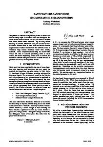
The goal of defining the error measures is to evaluate the performance of the segmentation system as a function of various parameters of the system. In order to achieve this the error measure must be monotonic. Given a reference video R and a comparison video V, the error measure e should be a monotonic function of the actual error, as V moves away from R, e should increase. The boundary error measure was applied to a set of simulated videos to verify these properties. The reference video contained 32 equal segments. The under segmented videos were generated by deleting segments from the reference videos while keeping the length constant. The over-segmented videos were generated by adding segments to the reference video without changing the locations of existing segments. Figure 8 shows the variation of the segment boundary e r r o r across the set of simulated videos. The plot shows the error as a function of the number of segments in the video. The error is zero at the location of the reference video and monotonically increases as the comparison video gets increasingly under (over) segmented to the left (right) of the reference video location. This is the error measure used to evaluate the performance of the segmentation system in the next section.
8.
Experimental Results
This section reports on the experiments performed based on the techniques proposed in this paper. The goals of the experimental evaluation have been to study the performance of the detectors (sections 8.2, 8.3), to tabulate the performance of the overall segmentation system (section 8.4) and to analyze the sensitivity of the entire system to variations in the threshold (section 8.5). The experimental results presented in here are a snapshot of
34
ARUN HAMPAPUR, RAMESH JAIN AND TERRY E. WEYMOUTH
f
Error Measures in Video Segmentation
B~ i h,
Error Measure
Under Segmented