PROFILE A GIS/Simulation Framework for Assessing Change in Water ...

DOI: 10.1007/s00267-0003-5 PROFILE A GIS/Simulation Framework for Assessing Change in Water Yield over Large Spatial Scales DALE D. HUFF WILLIAM W. HARGROVE ROBIN GRAHAM* NED NIKOLOV M. LYNN THARP Environmental Sciences and Computational Physics and Engineering Divisions Oak Ridge National Laboratory P.O. Box 2008 Oak Ridge, Tennessee 37831-6038, USA ABSTRACT / Recent legislation to initiate vegetation management in the Central Sierra hydrologic region of California includes a focus on corresponding changes in water yield. This served as the impetus for developing a combined geographic information system (GIS) and simulation assessment frame-

Millions of hectares of dry coniferous forest in the western United States are at risk for catastrophic crown fires because of structural changes (shifts in species and crown density) that have developed as a result of effective fire suppression since the early 1900s (Sampson 1997). Mechanical thinning is one management tool that can be used to control catastrophic fire risk and move the forest back towards its historic fire-resilient state. However, mechanical thinning produces large quantities of wood and bark that must generally be removed from the forest. The fate of this material is problematic, for in many cases the material is not suitable for conventional wood products (lumber or chips) and/or there is no local wood-products industry. Many parties are exploring novel uses of this material. One proposed use is as feedstock to produce bioenergy. Producing bioenergy either in the form of ethanol or power is an attractive option since these markets are large enough to absorb the quantities of material that would be generated if thinning was used to reduce the regional risk of fire. Furthermore, the production of bioenergy from this material has air quality and greenhouse gas benefits especially in comparison to prescribed burning or crown fires. KEY WORDS: Water-yield change; Forest management; GIS; Simulation; Monte Carlo Analysis *Author to whom correspondence should be addressed.

Environmental Management Vol. 29, No. 2, pp. 164 –181

work. Using the existing vegetation density condition, together with proposed rules for thinning to reduce fire risk, a set of simulation model inputs were generated for examining the impact of the thinning scenario on water yield. The approach allows results to be expressed as the mean and standard deviation of change in water yield for each 1-km2 map cell that is thinned. Values for groups of cells are aggregated for typical watershed units using area-weighted averaging. Wet, dry, and average precipitation years were simulated over a large region. Where snow plays an important role in hydrologic processes, the simulated change in water yield was less than 0.5% of expected annual runoff for a typical watershed. Such small changes would be undetectable in the field using conventional stream flow analysis. These results suggest that use of water yield increases to help justify forest-thinning activities or offset their cost will be difficult.

Because of its interest in bioenergy, the US Department of Energy (DOE) is supporting research and assessments of the technical, economic, and environmental feasibility of relying on forest thinning to reduce fire risk as a feedstock source for bioenergy. This paper describes the DOE-sponsored development and application of a framework for assessing the potential effect of thinning western coniferous forest on water yield at a regional (1000⫹ sq km) scale. Water yield effects were of particular interest to DOE because of their important energy, environmental, and economic implications. Water is often the most valuable commodity coming out these regions. Altering forest canopy through thinning could change evapotranspiration and thus water yield, and although mechanical removal of biomass for reduction of fire risk and production of bioenergy may not be economically attractive on its own, benefits such as increased water yield could improve its economic viability. The framework described here, while developed to be applicable across the west, was targeted towards understanding the water yield implications of widely applying a forest fire reduction strategy considered in the Herger-Feinstein Quincy Library Group Forest Recovery Act (US DOI 1998). This act, passed and signed into law in October 1998 as part of the omnibus budget bill, is “. . . a community stability plan to promote ecologic and economic health for certain Federal Lands and communities . . .” in the Sierra Nevada mountains ©

2002 Springer-Verlag New York Inc.

Assessing Change in Water Yield

165

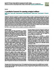
Figure 1. The study area evaluated for change in water yield as a result of forest thinning. Highlighted areas were excluded from consideration. California watersheds were used to aggregate area-weighted results.

in California. The act sets forth activities for fuelbreak construction, thinning of selected forest areas, and riparian management and restoration. Our goal was an assessment-level examination of the change in water yield that might result if the fire reduction management treatments proposed in the act were applied across the entire 42,000 sq km study area. Specifically, two thinning treatments, group selection (the harvest of clusters of trees) to reduce crown density to a fire resilient-level and the creation of defensible fuel profile zones (areas thinned to a very open canopy) along ridges were addressed. We wish to note that the management scenario we model differs significantly from the actions described in the act. The act considers only public lands and targets treating up to 283 sq kms (70,000 acres) of forest each year for five years. While we use two management treatments proposed in the act, we apply these treatments to all private forestlands

in addition to all the public lands considered suitable for treatment in the act. Thus we treat a much larger area and examine the implications of full-scale implementation of forest thinning to reduce the risk of catastrophic fire on regional water yield. We do not, however, include any public lands (such as wilderness or national parks) that are excluded in the act. Figure 1, developed in part from data provided by the Quincy Library Group (QLG) and Vestra Resources of Redding, California, USA, shows the total area we evaluated, excluded areas and California watersheds. To address the water yield changes associated with the regionally applied thinning treatments, we adapted an assessment model developed for silvicultural management (Troendle 1979) for use with a geographic information system (GIS) and applied this model to the study area shown in Figure 1. As

166

D. D. Huff and others

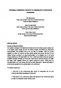
Figure 2. A combined GIS/simulation model framework for analyzing change in water yield from large-scale forest thinning.

part of the assessment, we developed a new leaf-area index map to characterize the forest vegetation. Because of the large area to be evaluated (approximately 42,000 sq km), some innovation was required to reduce computations. An important objective was to estimate the expected statistical range of response, rather than produce a single result. Consequently we used an efficient, systematic sampling method, Latin hypercube sampling (Iman and Helton, 1985). More specifically, the PRISM program (Gardner and others 1983) was used to generate multiple model-input files for a modified Monte Carlo simulation analysis. The results could then be used to evaluate mean response and variance of change in water yield. The method also includes area averaging to represent results for watershed accounting units, where not all of the forested area is treated. This approach allows an assessment at several scales and produces representative results for each of those scales. A qualitative examination of dominant seasonal patterns in evapotranspiration changes was also included.

Assessment Framework Because of the size of the QLG study area, the framework that was selected draws upon use of a geographic information system (GIS) and data derived in part from remote sensing. Mauser and Schadlich (1998) suggest that although there are current limitations to such an approach, it holds considerable promise for the future as new sensors

and instruments for data collection evolve. These developments, together with the summarizing and visualization power inherent in GIS, argue that this combination of remote sensing and GIS will continue to grow in power as more refined data become available and computing speed and memory capacity improve. Current emphasis on development of general circulation models that include feedback between the atmosphere and landscape, via soil–vegetation– atmosphere transfers (Avissar 1998), also supports the likelihood of improved capability to use a GIS/ remote sensing system to explore water resources issues. Avissar (1998) points out that such systems will probably be most effective if they focus at the scale of the problem from the outset, rather than attempting to scale up from individual plot-sized field experiments. Regardless, it is apparent that the GIS/remote sensing framework also must include a modeling interface to allow quantitative assessments. Figure 2 shows the elements of our assessment framework and summarizes the process of model application and analysis. The framework suggested here can be visualized as a three-part system: (1)

study definition and model selection (step 1), followed by assembly and manipulation of spatially-distributed data (GIS data layers) to generate input files for the hydrologic simulation model (step 2); (2) modified Monte Carlo simulations of expected change in water yield resulting from forest man-

Assessing Change in Water Yield

agement practices to produce location-specific results for statistical summary (step 3); and (3) analysis and spatial (GIS) display of results for evaluation and interpretation (step 4). Results may suggest repeating the steps with different data or models (step 5). The following discussion illustrates application of the assessment framework, following the sequence of steps shown in Figure 2.

Application of the Framework Study Definition Simply stated, if it were possible to go from current forest conditions to a more open, fire-resistant situation, how much would water yield change? To address this question, we assumed that vegetation removal for fire suppression would be a combination of group selection and fuel breaks. We ignored access road issues. The goal was to explore the overall potential for water yield changes for a large enough area to be representative if a fire-suppression management plan like the one proposed by the QLG were fully deployed at a regional scale. Model Selection To estimate change in water yield from vegetation management, actual evapotranspiration must be related to the change in vegetative characteristics. The simplest way is through regression models (Douglass and Swank 1975), where factors like fractional reduction in basal area and the insolation index are used to estimate annual change in runoff. This approach requires observations from paired watershed studies for a range of representative conditions. Evaluations using this approach for the Sierra Nevada have been completed recently (Marvin 1996, Kattleman 1996). Alternatively, simulation of actual evapotranspiration and runoff, using physical, climatic, and vegetative properties can be used to derive change in water yield (defined as the difference between precipitation and actual evapotranspiration). Huff and Swank (1985) describe an example of this latter approach, applied to a long-term clear cutting and regrowth experiment at the Coweeta Hydrologic Laboratory in western North Carolina. However, as the complexity of the method increases, data requirements become more difficult to satisfy, making large-scale applications of more detailed models impractical. An intermediate strategy uses calibrated simulation models with field observations to extend the

167

experimental evidence. We also chose to emphasize change in water yield caused by forest thinning, rather than the absolute annual total. Huff and Swank (1985) concluded this measure was more reliably achieved. This approach allows development of simplified relationships to forecast expected change in runoff from forest manipulation (Troendle 1979). Because of simpler data requirements for this methodology, we chose this approach and, specifically, the Forest Service Water Resources Evaluation of NonPoint Silvicultural Sources (WRENSS) assessment model (US EPA 1980). The Forest Service (WRENSS) methodology was originally published in the form of an assessment handbook (US EPA 1980). The portion dealing with changes in annual water yield was converted to a computer program to facilitate its use and has continued to evolve (Bernier 1986, Swanson 1991). A modified version of the Fortran program was developed for our analysis (Huff and others 1999) for use on a workstation where it could interface directly with GIS data. Details of the WRENSS model and its data requirements are discussed in Huff and others (1999), and hence are not repeated here. However, to aid understanding we include some discussion of parameters that exert the most control on change in water yield, as well as supplemental information on data sources used for the application presented here. Spatial Resolution The minimum spatial resolution is important for any GIS analysis. Since we planned multiple model runs to assess water yield and its variability and the study area was about 42,000 km2, we chose a 1-km map cell resolution. This choice allowed use of readily available data sets for the large number (⬎192,000) of simulation runs needed. Reducing the cell size further would have complicated the development of data and increased the number of simulations required. This seemed inappropriate for the initial application of our assessment framework. Data Needs. Topography. The WRENSS model differentiates between two types of watershed units, snow-dominated and rain-dominated. Where a snow pack affects hydrologic processes, the areas are called “snow-dominated process” (SDP) units. The other type of watershed includes “rain-dominated process” (RDP) units. Ideally, differentiation between SDP and RDP units is based on hydrograph response for any given unit. However, we used elevation as a surrogate for available energy and climatic conditions, hence as a means to divide SDP

168

D. D. Huff and others

and RDP units in our large-scale assessment. We used a digital elevation model (GTOPO30 2000)) to define the aspect for each type of unit. We also used elevation to estimate the energy-level for each snow-dominated cell. The energy level controls, in part, the amount of water lost from the unit to evapotranspiration or snowpack sublimation. SDP units are further differentiated by an energy aspect, i.e., a combination of slope face direction and elevation. The energy-aspect classification modifies the total seasonal water loss for any SDP unit. Because WRENSS is an annual model that uses seasonal estimates of total runoff, there is no attempt to estimate timing of runoff from either snowmelt or direct precipitation. Based on discussion with local foresters, sites below an elevation of 610 m were assigned a RDP hydrologic response. The high-energy level classification for SDP units was assigned to elevations between 610 and ⬎1220 m above mean sea level. Intermediate and lowenergy levels were assigned to SDP units with elevation 1220 m above sea level. Further details, including rules used to assign aspect or facing direction to units, are given in Huff and others (1999). Seasonal precipitation. WRENSS divides the annual cycle into seasons, which vary in number depending on the location of the study area. For the WRENSSdefined Central Sierra hydrologic region (region 7), four seasons are used (US EPA 1980). Seasonal precipitation, together with time of year, is used to estimate a corresponding baseline evapotranspiration value. For SDP units, where snow pack plays a significant role, the model has the capability of adjusting evapotranspiration for the effects of snow redistribution. However, in the Central Sierra, where wet snow conditions prevail, the WRENSS handbook recommends not to use the redistribution feature (US EPA 1980). Seasonal precipitation totals were constructed from the monthly values contained in a statistical–topographic model for mountainous terrain (Daly and others 1994). These totals represent synoptic conditions. To explore wetter and drier years, precipitation was increased to 150% of average to represent a wet year and decreased to 65% of average for the dry year case. These adjustments were selected from water year precipitation summaries (1983–1998) available through the California Department of Water Resources (2000) web site. The Sacramento River Basin data were used, and the values were selected to stay within observed ranges in precipitation (173% of average for a wet year and 56% of average for a dry year) over the past two decades, although there were a few wetter and a few drier years. Because of our focus on annual change in

water yield, rather than actual runoff, we believe this is acceptable. Vegetative characteristics. WRENSS characterizes vegetation by dominant tree species and vegetation cover density. Unfortunately, the coefficients that define WRENSS options for dominant tree species are limited by data availability in region 7 (Central Sierra). In the snow-dominated regions of the study area, we used the “lodgepole pine” option because data to support the Ponderosa pine option are not available. In the rain-dominated areas we used the “conifer” option. WRENSS uses plant/tree species and either leafarea index (RDP sites) or basal area (SDP sites) to characterize the vegetative cover density. Leaf-area index (LAI) is the ratio of (one sided) leaf surface area per unit underlying ground surface area. Basal area is the total cross section of tree stems, generally at breast height and inclusive of bark, per unit surface area. We developed a new 1-km-resolution spatial data set of maximum projected one-sided LAI for the entire study area, then used LAI to estimate basal area for SDP units. The LAI data were developed in a three-step procedure using 1-km-resolution Advanced Very High Resolution Radiometer (AVHRR) data provided by the NOAA/NASA Pathfinder program, together with a digital elevation model. In the first step, a greenness index was computed as the ratio of the near infrared to the red reflectance value for each AVHRR map cell. The greenness index was computed for 11 different composite periods during the growing season. Next, the greenness index was used to estimate LAI by inverting a mechanistic radiative transfer model of the canopy. This model accounts for effects of sensor view angle, solar elevation, leaf optical properties, background reflectance, canopy leaf angle distribution, and foliage clumping on the bidirectional reflectance above the canopy (Nikolov 1998). Finally, the maximum LAI from the 11 estimates was used to represent the optimal seasonal LAI for each map cell (Figure 3). The original WRENSS model uses the total as opposed to the projected leaf surface area in its relationships. We adapted the model coefficients to allow direct use of projected LAI for RDP units. We transformed total leaf surface area to projected LAI by dividing by a factor of 2.5, a compromise between flat leaves, which have a conversion factor of 2.0 (surface to projected area) and rounded conifer needles, which have a conversion factor of 2.8 –3.2 (Johnson 1984). For SDP map cells (above 610 m elevation), the

Figure 3. Estimated maximum leaf-area index values within the study area. Map cell resolution is 1 km on a side.

Assessing Change in Water Yield

169

170

D. D. Huff and others

optimal seasonal LAI was transformed to basal area using the following equation: Basal area ⫽ (a ⫹ b 䡠 LAI) 䡠 LAI where a ⫽ 20.33 and b ⫽ ⫺ 1.31 and basal area is given in units of square meters per hectare. This relationship was developed using literature values relating surface leaf area or projected leaf area to basal area in ponderosa pine dominated stands (Gholz 1982, Runyon and others 1994, Whittaker and Neiring 1975, Gholz and others 1976); published allometric equations relating Ponderosa pine, true fir, and Douglas fir foliage mass to tree diameter at breast height (dbh) (Gholz and others 1979, Waring and others 1978, Cable 1958, Kittridge 1944); literature values on projected or total leaf surface area per unit foliage mass (Pierce and others 1994, Cable 1958); and forest inventory data from the Plumas and Lassen national forests. Literature values present an inconsistent or incomplete picture of the relationship between basal area and leaf surface area. Allometric equations differed by almost a factor of two in their projections of leaf mass for the same size ponderosa pine tree. Thus considerable professional judgement was exercised in developing this relationship. In the RDP areas, WRENSS also requires an estimate of relative rooting depth. This parameter is a measure of the water-holding capacity of the rooting zone. To estimate this depth parameter, we used a GIS coverage that provides a measure of plant-available water capacity (National Cartography and GIS Center 1991). The integrated capacity to a depth of 1.5 m, expressed as a depth of water per unit area of soil, is related to soil depth through a measure of the fractional volume of water between field capacity and wilting point. We assumed a typical moisture-content range between field capacity and wilting point of 0.1 m3/m3 (Huff and others 1999). Thus, the plant-available water may be scaled to an equivalent rooting depth of soil by multiplying it by 10. Vegetation management scenario characterization. The area shown in Figure 1 (42,067 km2) was the starting point for the analysis. Areas of nonforest vegetation were removed, reducing the available area to 22,122 km2. Existing wilderness, off base (e.g., proposed wilderness additions), deferred (i.e., areas of special concern such as botanical areas), lakes, areas north of Highway 299, or areas in Blacks Mountain or Swain Mountain were excluded, which further reduced the area eligible for thinning to 16,662 km2. Vegetation cover density, as indicated by the LAI data, was the final factor in determining the final number of map cells eligible for thinning. Application of minimum

LAI requirements (LAI ⬎ 2) reduced the total number of eligible map cells to a total of 6451. Most (6304) were in SDP areas. There were 3991 lowenergy SDP cells and 2313 higher-energy SDP cells that were eligible to be thinned. There were relatively few RDP map cells (147). All remaining map cells were excluded from consideration by the management plan or had vegetative cover that fell below the thinning threshold. For all the excluded map cells, the change in water yield is zero, since no changes in vegetation (and corresponding evapotranspiration) occur between pre- and posttreatment conditions. To define the effect of thinning for fuel reduction on posttreatment vegetation density, we assumed that map cells selected for group (or individual tree) selection would have a postharvest LAI of 2.0 or a basal area of 34.4 m2/ha (150 ft2/acre), composed primarily of large-diameter trees. Sensitivity analyses showed results that were more sensitive to the thinning threshold than to the basal area conversion equation. The actual number of map cells meeting the criteria for group or individual tree selection was 3248. Most of the 1-km map cells were likely to contain a mixture of various forest cover densities and nonforest conditions (roads, towns, clear-cuts, etc.). Thus map cells that are not thinned in our analysis (because their initial LAI is less than 2.0) could well include some forest stands that have a leaf area index greater than 2.0. These stands would be thinned if the spatial resolution of the data were finer. Thus our estimate of reduction in vegetation density is conservative and may underestimate the land area that would be thinned. To represent fire breaks, which are termed defensible fuel profile zones (DFPZ), we assumed forests along watershed boundaries (ridge lines) would be thinned to an LAI of 1.5 or a basal area of 27.5 m2/ha (120 ft2/acre) in a 100-m-wide swath. Estimating the change in water yield for vegetation removal to create defensible fuel profile zones was a challenge, since the spatial scale associated with the DFPZ areas is smaller than the 1-km resolution used for the rest of the analysis. Instead of using finer spatial resolution, an empirical target basal area that generated approximately the same change in water yield was derived. The targets for thinning in DFPZ map cells were established as 31.3 m2/ha (equivalent LAI of 1.71) for low-energy SDP map cells, 31.5 m2/ha (equivalent LAI of 1.72) for higher-energy SDP map cells, and a LAI of 1.88 for RDP map cells. The 3203 map cells were thinned using the DFPZ criteria. Pre- and postthinning leaf-area index distributions for the map cells selected from the vegetation manage-

Assessing Change in Water Yield

Figure 4. The pre- and postthinning leaf area index (LAI) distributions among all map cells that had simulated thinning.

ment criteria are shown in Figure 4. The effect of the vegetation management scenario was to reduce vegetation density for all map cells with LAI ⬎ 2.0 for group selection or 1.8 for DFPZ thinning. Thus, the postthinning distribution shows increased frequencies in the LAI ⫽ 2.0 and LAI ⫽ 1.8 categories to reflect the reductions in higher LAI categories. The same assessment framework could be used to evaluate other treatment scenarios.

171

indicated that retention of three principal components was most appropriate. Factor scores for each map cell were submitted to a clustering procedure (SAS Institute 1985) using the k-means algorithm (MacQueen 1967). Each of the six possible elevation/aspect combinations for SDP cells, and the RDP map cells were clustered separately, resulting in clusters that contained cells of only a single elevation/aspect class. To ensure uniform and comparable within-cluster hydrologic heterogeneity, the maximum radius for clusters in data space was specified rather than the explicit number of desired clusters. Thus, more hydrologically heterogeneous elevation/ aspect combinations were divided into more clusters in a way that was driven by the data. Finally, all map cells were merged, and clusters were renumbered by ascending elevation/aspect class. The end result was 586 SDP clusters and 56 RDP clusters. Characterization of Cluster Statistical Properties The statistical characteristics (mean, standard deviation, maximum and minimum values for each input variable) for each cluster were determined from an analysis of the GIS data for all map cells within that cluster. These spatial statistics within each cluster provided the basis for generating input data files in the subsequent analysis. Generation of Model Input

Managing the Data to Condense the Problem Grouping Similar Landscape Cells To reduce the number of individual simulation runs and obtain a measure of likely variability of results, geographic multivariate cluster analysis (SAS Institute 1985) was used. The objective was to group all eligible map cells with similar model input parameters into clusters. Rather than dividing the mountainous Quincy area geographically into contiguous subregions for simulation, we employed a purely statistical clustering of map cells based on the multivariate hydrologic characteristics of each cell (i.e., the input variables for the WRENSS model). The clusters that resulted were spatially disjoint but were collections of cells with similar physical, hydrologic, forest type, and vegetation characteristics. RDP cells underwent separate principal component analysis (PCA), since RDP input variables included pre- and postthinned LAI and were thus different from SDP units. In addition, RDP units also have a relative root depth parameter that was considered. After orthogonal equamax axis rotation, scree plots of eigenvalues for both RDP and SDP clusters

To preserve the spatial variability in hydrologic characteristics, we simulated water yield change for each cluster by using 100 independent WRENSS simulation runs. We employed Latin hypercube (LH) sampling (Iman and Helton 1985) to construct WRENSS input data sets based on the statistical characteristics previously defined for each cluster. LH sampling divides the range of each input parameter into equal probability class intervals and ensures that the entire range of each parameter will be well represented with fewer samples than random Monte Carlo simulations would require. In addition, the type of frequency distribution for each variable was also specified. The PRISM program (Gardner and others 1983) created 100 different model input data sets (realizations) for each cluster. This statistically representative distribution of input data sets allows calculation of a distribution of simulated hydrologic outputs. Rather than a single result, a mean and variance of simulated hydrologic response was produced for each cluster. Thus, all cells in each cluster have the same mean and variance for the simulated change in water yield. Parameters that were allowed to vary among input data sets included seasonal precipi-

172

D. D. Huff and others

tation, pre- and postthinning vegetation cover (LAI or basal area), the parameter describing cover density when evapotranspiration reaches the potential value (SDP units only), and the rooting depth parameter (RDP units only). A potential problem was identified during the course of doing the simulation studies. Each cluster has a pretreatment and posttreatment distribution for LAI or basal area. However, if there is overlap between the distributions, it is possible for pre- and posttreatment values selected by the LH method to cross over. This results in the highest LAI or basal area being assigned to the posttreatment input data set. Physically, the overlap represents a fraction of the map cell that would not be thinned because vegetative cover density is below the treatment threshold. We simply set the posttreatment value equal to the pretreatment value for these situations.

Simulating the Results Multiple Model Runs For each of the 495 SDP clusters, three different scenarios (average, wet, and dry annual precipitation conditions) involving 100 simulations each were completed. For RDP clusters, model results are not affected by varying precipitation amounts, so only the average annual precipitation case was simulated. Statistical properties (mean and variance) of the change in water yield were determined and saved for later export to the GIS data set. Simulations (163,200 individual model runs) took about five days of machine time on a 300MHz DEC Alpha workstation.

Surprisingly, the original WRENSS model predicted a net loss in water yield for thinning on many SDP clusters. The model was originally developed from field results for clear-cutting experiments when experimental data for thinning only were not available. Subsequent studies (Troendle 1987) indicate that thinning significantly reduces winter interception loss and may also reduce summer soil water depletion, at least in wet years. This result would argue that a net loss in water yield associated with thinning is unlikely. To evaluate both the original WRENSS model and results supported by later studies, we also allowed for the possibility that in any season where the original model shows a net loss in water yield following thinning, the seasonal change in water yield could be zero. Thus we created two sets of results. The adjustment may underestimate actual gains but is supported by current understanding (C. A. Troendle, personal communication 1999). Table 1 is a summary of simulated change in water yield for the various scales that were considered. The original model simulation results are shown, along with values that were modified to correct for the new information on thinning. The recompiled results are shown in the “adjusted” column and are referred to hereafter as adjusted values. The net effect was to increase the mean water yield for the average treated cell by about 3.2 mm. Since negative values were removed, the range decreased and there was also a slight drop in the associated standard deviation. Although we believe the adjusted values best represent the change in water yield for the scenario presented, we also show the original model results for comparison. Individual Cell (Cluster) Results

Summary of Results: Change in Water Yield We explored the potential changes in water yield (upper limits) that could result from complete implementation of the philosophy included in the Quincy Library Group Forest Recovery Act. This assumption narrows the focus to the effects of the vegetation manipulation, and eliminates the influence of annual variations in precipitation. We examined average, dry, and wet years, and report the corresponding changes in water yield for those scenarios. The results are strongly dependent on the scale of the reporting unit. We have chosen to summarize results at three different scales: (1) (2) (3)

individual map cells, watersheds (California watersheds on the QLG Community Stability Proposal/Vestra map), and USGS hydrologic units (see the USGS 2000).

RDP map cell results show the largest changes in water yield as a result of thinning. For all cells that were treated, the overall uncorrected change in water yield was ⫹ 2.0 ⫾ 14.5 mm for a year with average precipitation. The range across all treated cells was ⫺15.4 to ⫹ 165.6 mm. After adjusting the negative seasonal values to zero, the mean response was ⫹5.2 ⫾ 13.7 mm and the values ranged from 0.0 to 165.6 mm. Similar changes occurred when the cells were subdivided into the three dominant types of WRENSS units (SDP low energy, SDP intermediate to high energy, and RDP). There is a clear progression of increasing yield as one moves to situations where more energy is available for evapotranspiration (Table 1). Frequency distributions, showing the number of cells associated with different annual change in water yield values (Figure 5), provide insight on the cell results presented in Table 1. The

Assessing Change in Water Yield

Table 1. unitsa

Summary of annual change in water yield for average conditions for cells, watersheds, and hydrologic

Original model

Description All thinned cells

Number of units 6451

SDP low energy cells

3991

SDP higher energy cells

2313

RDP cells Thinned California watersheds (cells)

147 16973

Thinned hydrologic units (cells)

46969

Larger water accounting units Thinned California watersheds

Thinned hydrologic units

a

173

429

15

Type year

Change mean (⫾ standard deviation, mm)

Dry 1.60 ⫾ 14.35 Average 1.99 ⫾ 14.48 Wet 2.08 ⫾ 14.62 Dry ⫺1.37 ⫾ 0.14 Average ⫺1.19 ⫾ 0.16 Wet ⫺1.34 ⫾ 0.17 Dry 1.54 ⫾ 0.15 Average 2.31 ⫾ 0.19 Wet 2.84 ⫾ 0.21 All 83.0 ⫾ 1.01 Dry 0.61 ⫾ 0.04 Average 0.75 ⫾ 0.05 Wet 0.79 ⫾ 0.05 Dry 0.22 ⫾ 0.015 Average 0.27 ⫾ 0.017 Wet 0.28 ⫾ 0.018 Dry Average Wet Dry Average Wet

0.82 ⫾ 3.60 1.01 ⫾ 3.66 1.07 ⫾ 3.77 0.46 ⫾ 0.68 0.54 ⫾ 0.72 0.56 ⫾ 0.72

Adjusted model (nonnegative change in seasonal water yield)

Range (mm)

Change mean (⫾ standard deviation, mm)

⫺14.4–165.6 ⫺15.4–165.6 ⫺16.4–165.6 ⫺13.7–6.9 ⫺15.4–6.9 ⫺16.4–7.0 ⫺4.9–6.9 ⫺4.9–7.8 ⫺4.9–8.2 11.1–165.6 ⫺14.4–165.6 ⫺15.4–165.6 ⫺16.4–165.6 ⫺14.4–165.6 ⫺15.4–165.6 ⫺16.4–165.6

4.6 ⫾ 13.6 5.2 ⫾ 13.7 5.5 ⫾ 13.7 2.89 ⫾ 0.11 3.40 ⫾ 0.14 3.62 ⫾ 0.15 2.54 ⫾ 0.14 3.30 ⫾ 0.18 3.84 ⫾ 0.20 83.0 ⫾ 1.01 1.74 ⫾ 0.03 1.97 ⫾ 0.04 2.09 ⫾ 0.05 0.63 ⫾ 0.012 0.71 ⫾ 0.015 0.76 ⫾ 0.012

⫺5.2–33.9 ⫺5.3–34.2 ⫺5.8–34.4 ⫺0.11–1.95 ⫺0.09–2.07 ⫺0.10–2.06

2.10 ⫾ 3.30 2.37 ⫾ 3.36 2.53 ⫾ 3.41 0.98 ⫾ 1.03 1.09 ⫾ 1.11 1.15 ⫾ 1.15

Range (mm) 0.0–165.6 0.0–7.63 0.0–7.67 0.0–7.67 0.0–6.91 0.0–7.85 0.0–8.57 11.1–165.6 0.0–165.6

0.0–165.6

0.0–34.4 0.0–34.6 0.0–34.9 0.001–3.35 0.002–3.56 0.002–3.65

Where a single range is given, all ranges are the same.

adjusted SDP map cell values generally range from 0 to 7 mm, with a mean of about 3.4 mm. Note that about half of all treated SDP map cells show no change in annual water yield. The other half show an increase mostly between 6 and 8 mm. The RDP cells show a range for change in water yield between 11 and 166 mm, with a mean value of about 83 mm. Even though RDP map cells represent only about 2% of all thinned areas, they contribute nearly one third of the average change in water yield across all treated map cells (Table 1). Statistical Summary of Basic Results (Adjusted Values) Spatial aggregation of results. Figure 6 shows a map of adjusted water-yield changes by individual map cell for the entire study area. The patterns suggest that DFPZ cells along watershed boundaries were responsible for most of the change in water yield. The cells from the middle of the watershed units (group and individual tree selection cells) mostly showed no change in water

yield for the example scenario. Based on a combination of Figures 5 and 6, it appears that the group selection map cells generally contribute zero change in water yield and the DFPZ map cells contribute the positive changes. This result clearly suggests that the threshold for positive change in water yield for SDP units is between LAI (and associated basal area) values of about 1.8 and 2. Aggregation to California watershed scale. As the area increases, the mean change in water yield diminishes. All California watersheds where at least one cell within the basin was thinned (429 watersheds out of 936 in the study area) were considered. There are two ways to calculate statistics for these units: area-weighted values for all cells, and even-weighted values by aggregated watershed. In the top portion of Table 1, the mean area-weighted adjusted change in water yield in a typical map cell (for all California watersheds) was calculated by summing values for all cells in the area and dividing by the total number of cells (Huff and others 2000). To determine the standard deviation for the

174

D. D. Huff and others

adjusted change in annual water yield was 1.97 ⫾ 0.04 mm. In the lower portion of Table 1, the even-weighted values by watershed are given. They represent the mean and standard deviation of the 429 individual watershed area-weighted values. The mean value for an average precipitation year was 2.37 ⫾ 3.36 mm, with a range of 0 –34.6 mm between the lowest and highest watershed. This latter value represents the typical variability among individual watersheds. The spatial distribution of wateryield changes in the study area is shown in Figure 7. The associated frequency distribution of change in water yield for the 429 watersheds that contained at least one thinned map cell is shown in Figure 8. Hydrologic units. Fifteen US Geological Survey hydrologic units (HUCs) contained at least one treated cell. The average (area-weighted) change in water yield for a typical cell within the full area of all 15 units (46,969 cells) was 0.71 ⫾ 0.015 mm, with a range between 0 and ⫹165.6 mm. The even-weighted mean and standard deviation for the 15 hydrologic units (average size was 3130 cells) for an average year was 1.09 ⫾ 1.11 mm. Note that we use the same assumptions as described for California watershed calculations to determine the error terms for typical cells in hydrologic units, except Nw becomes the number of cells in all 15 hydrologic units. The spatial distribution of water yield changes by USGS HUC is shown in Figure 9. Figure 10 displays the frequency distribution of water-yield changes for the 15 HUC areas that contained at least one map cell where forest thinning was simulated.

Figure 5. The frequency distribution of change in water yield at the individual cell level for each hydrologic regime that was modeled. Nearly half of all cells that were thinned showed no change for average annual conditions.

area-weighted change in water yield, we used a weighting factor (Nc/Nw), where Nc is the number of treated cells in a cluster and Nw is the total number of cells in all watersheds; the variance for each cell in the cluster; and a covariance term, which reduces to zero if the variances are uncorrelated (Snedecor and Cochran 1982). We have assumed that the clustering process renders the cells in each cluster essentially independent from cells in other clusters. Thus, we obtain the area-weighted variance as the sum of the product of the square of the weighting factor and variance over all clusters in the watershed. The standard deviation is shown in Table 1. The area-weighted values correspond to the average cell within the entire extent of all treated watershed areas (16,973 cells). For this analysis, the

Evaluation Sensitivity of Change in Water Yield to Model Parameters The PRISM program (Gardner and others 1983) was used for a sensitivity analysis of randomly selected RDP and SDP clusters. The analysis included 13 input parameters for the RDP clusters and seven input parameters for the SDP clusters. For the RDP clusters, variables included in the analysis were seasonal precipitation values (four values), seasonal values for LAI both before and after thinning (eight values), and rooting depth (one value). For the SDP clusters, the variables included seasonal precipitation (four values), pre- and postthinning basal area (two values), and a parameter (one value) that describes the limiting basal area above which evapotranspiration will be at the potential limit. Input data sets for the sensitivity analysis were generated from a normal distribution for the selected input parameters using 500 equal-probability class intervals, and each parameter was varied ⫾1%

Assessing Change in Water Yield

175

Figure 6. The spatial distribution of change in water yields by individual map cell within the study area. The simulated defensible fuel profile zones (DFPZ), which were assumed to follow watershed boundaries, are clearly evident.

about its mean value. Sensitivity indices ranked the input parameters having the most influence on change in water yield. Results are presented in Table 2. For SDP energy aspects, there are two basic patterns: Most of the low energy aspect clusters show slightly higher sensitivity to prethinning basal area than to postthinning basal area. The exception, cluster 15, has a lower initial value for basal area than the other clusters in this group and shows much higher sensitivity to postthinning basal area. For the higher energy aspect clusters, two of the three examples show the highest sensitivity to postthinning basal area and a secondary sensitivity to the parameter describing the basal area threshold where water use reaches its maximum value. Changes in evapotranspiration are primarily linked to vegetation cover density before and after treatment. In the rain-dominated process clusters, the primary sensitivities involve spring and winter season LAI. It may seem surprising that precipitation does not influence change in water yield. This result simply emphasizes the difference between change in water yield and total water yield. The latter is primarily affected by precipitation,

while the former depends almost entirely on changes in vegetation cover. Magnitude of Change in Water Yield The results suggest that it will be extremely difficult to use conventional methods (e.g., streamflow measurement analyses) to quantify changes in water yield resulting from forest thinning. Average expected annual runoff is approximately 600 mm for the study area (Kattelmann 1996). Even at the scale of a typical California watershed (⬃40 km2), the change in annual water yield under the modeled scenario is only about 0.3% of the typical total runoff (Table 2). Ziemer (1986) indicated that forest management for increased water yield is impractical, particularly at larger scales, and our results support that finding. Keppeler (1998) presents information on water yield response to timber harvest, although the harvest was primarily clear-cut rather than the thinning scenario we used. The range in values we observed, however, indicates that individual areas could

176

D. D. Huff and others

Figure 7. The spatial distribution of change in water yields by California watershed for average annual conditions. Only watersheds with at least one treated cell are shown.

nario by either the original or adjusted methods we used. Thus, the aggregation process, using areaweighted values, is an important aspect of the methodology because it allows estimation of changes in water yield that are smaller than could be detected by conventional flow measuring techniques. Seasonal Distribution of Changes

Figure 8. The frequency distribution of water-yield changes by watershed for an average annual precipitation pattern.

have significantly higher water yield compared to the average. Normal year-to-year variability that results from differing climatic conditions eclipses the increases in water yield simulated for the example sce-

To examine the seasonal timing of expected changes in water yield, two representative sets of cluster results (one SDP and one RDP) were compared. Both SDP categories were similar, so only one SDP example is shown. Figure 11 illustrates the seasonal distribution of adjusted net change in evapotranspiration for representative clusters from snow and rain dominated hydrologic regimes. Normalized values were obtained by taking the quotient of seasonal evapotranspiration and the annual total change. Similar normalized values of seasonal precipitation are shown.

Assessing Change in Water Yield

177

Figure 9. The spatial distribution of water-yield changes by USGS HUC. All shaded areas had at least one treated cell within their boundary.

Figure 10. The frequency distribution of water-yield changes by USGS HUC for average annual conditions.

In the SDP cluster (higher energy aspect; Figure 11), the most notable feature is that most (⬃70%) of the change in annual water yield (average value is 8.0 ⫾ 3.2 mm with a range of 0.1–12.9 mm) occurs during the summer season. Change in simulated seasonal water yield represents the difference between pre- and posttreatment evapotranspiration. During

summer it is more indicative of soil moisture content, although the relationship between soil moisture and stream flow is complex and nonlinear. A reduced summer soil-moisture deficit probably indicates earlier onset of runoff in the following water year, rather than increased summer flows. This result suggests a useful target (soil moisture changes and/or summertime low flow) for field studies to evaluate thinning operations for SDP units. There is a fairly uniform seasonal distribution of change in water yield for the RDP cluster (Figure 11). The selected cluster showed a net annual gain of 74.2 ⫾ 3.7 mm in water yield between pre- and posttreatment conditions. The range was 65.2– 85.0 mm, with the largest seasonal contributor in spring, even though most precipitation occurs in the winter season. RDP clusters represent a small fraction of all treated areas, but as indicated earlier, their impact on change in water yield at the watershed scale is significant. If RDP areas are included in vegetation management plans, conventional measurements to estimate change in water yield may be feasible.

178

Table 2.

D. D. Huff and others

Summary of water-yield changes versus WRENSS parametersa Results for snow dominated process clusters with low energy aspects

WRENSS Parameters Prethinning basal area Basal area at maximum water use Postthinning basal area Total explained change

Cluster 14 cells north aspect

Cluster 15 cells north aspect

Cluster 191 cells south aspect

Cluster 254 cells south aspect

Cluster 358 cells E/W aspect

57.6 2.2 40.3 100.1

0.8 20.0 79.3 100.1

57.2 0.8 42.3 100.3

55.3 3.6 40.9 99.8

57.8 1.3 41.0 100.1

Results for snow dominated process clusters with higher energy aspects Cluster 98 cells north aspect

Cluster 286 cells south aspect

Cluster 494 cells E/W aspect

56.8 0.7 42.9 100.4

0.0 17.1 83.0 100.1

0.0 17.8 82.3 100.1

Prethinning basal area Basal area at maximum water use Postthinning basal area Total explained change

Results for rain dominated process clusters

Fall prethinning LAI Winter prethinning LAI Spring prethinning LAI Summer prethinning LAI Fall postthinning LAI Winter postthinning LAI Spring postthinning LAI Summer postthinning LAI Total explained change a

Cluster 627 cells

Cluster 638 cells

Cluster 629 cells

7.0 12.6 18.1 3.7 9.4 10.1 37.0 3.1 101.0

0.3 10.1 27.7 0.1 10.1 9.5 39.0 4.2 101.0

7.4 11.5 23.3 1.9 8.9 9.6 35.3 3.0 100.9

Values indicate percentage of change in water yield attributed to the parameter indicated.

Implications for Monitoring Effect of Vegetation Management Hydrologic Issues Perhaps the most striking facet of this analysis is the effect of increasing scale, where the importance of excluded areas on achievable water yield becomes obvious. Most studies of forest thinning are done at a small plot or watershed scale. This approach is necessary to accurately quantify the changes. However, as the size of the area increases, and smaller fractions of the landscape are actually treated, the overall effect becomes more difficult to measure directly. At some point, the natural variability in annual precipitation patterns, coupled with the reduced average effect of thinning, will eliminate the opportunity to directly measure the response using stream flow. At that point, quantification must rely on aggregation of results from smaller, representative study areas. The analysis also shows that the most dramatic simulated gains in water yield occur in the RDP areas. Even though there were relatively few of them in our analysis,

the RDP areas may represent areas where effects of thinning would be most easily measured. It is also important to note that if the threshold elevation for separating RDP and SDP units was found to be too low, raising that elevation level would increase the number of RDP cells and probably cause a disporportionate increase in estimated average annual change in water yield for treated cells. Generality of Assessment Framework The methodology that was established for this evaluation is useful for structuring a systematic approach to a variety of issues. The example presented here illustrates that even a simplified scenario can yield useful insights for issues that involve a large area. The important contribution is in the framework and associated methods, rather than the specific example. The framework offers a powerful tool for future progress. It provides the opportunity to identify and assemble new spatial data sets and models for systematic evaluation of alternative management strategies.

Assessing Change in Water Yield

179

more refined data and models. Development of massively parallel computer models that link the terrestrial and aquatic systems in a three-dimensional representation and also allow greater temporal resolution are a worthy goal for the future. In such a context, the application framework presented here has utility for designing and testing alternative forest management scenarios on the entire ecosystem before they are implemented.

Acknowledgments The authors wish to thank Chuck Troendle for his assistance and suggestions on application of the WRENSS model. Bob Swanson also offered helpful suggestions and information. Virginia Dale and Chuck Garten provided helpful review comments and suggestions to improve the manuscript. In addition, John Ferrell of the US Department of Energy provided the encouragement and support needed to complete this project. Research was sponsored by the US Department of Energy, Bioenergy Feedstock Development Program. University of Tennessee–Battelle, LLC manages Oak Ridge National Laboratory for the US Department of Energy under contract number DE-AC05-00OR22725. Figure 11. The seasonal precipitation and change in water yield distributions, expressed as a fraction of total annual change, for representative groups of cells for snow- and raindominated areas.

The effects of large-scale vegetation management are difficult to evaluate, particularly when it is desirable to have multiple benefit targets (i.e., fuel reduction, bioenergy development, fire risk, water quality, and quantity changes). The general approach embodied in the framework presented here can be useful for addressing a variety of questions systematically. It need not be confined to water-related issues. By substituting other models and other spatial data, a broad variety of issues can be addressed. Finally, the spatially explicit organization of information that is inherent in GIS data sets can provide a guide for gathering and organizing data. For example, reliability of change in water yield estimates could be improved with refined basal area information, as well as more a explicit description of vegetation species. Thus the example analysis provides a guide for future data synthesis. An important part of this synthesis depends on the spatial resolution and models used in the analysis. Evaluation of effects of vegetation management on timing and water quality of stream flow will require

Literature Cited Avissar, R. 1998. Which type of soil-vegetation-atmosphere transfer scheme is needed for general circulation models: A proposal for a higher-order scheme. Journal of Hydrology 212–213:136 –154. Bernier, P. Y. 1986. A programmed procedure for evaluating the effect of forest management on water yield. Forestry Management Note No. 37. Northern Forestry Center, Canadian Forestry Service, Edmonton, Alberta, 12 pp. Cable, D. R. 1958. Estimating surface area of ponderosa pine foliage in central Arizona. Forest Science 4(1):45– 49. California Department of Water Resources. 2000. http:// cdec.water.ca.gov/cgi-progs/previous/PRECIPOUT Daly, C., R. P. Neilson, and D. L. Phillips. 1994. A statistical– topographic model for mapping climatological precipitation over mountainous terrain. Journal of Applied Meteorology 33:140 –148. Douglass, J. E., and W. T. Swank. 1975. Effects of management practices on water quality and quantity: Coweeta Hydrologic Laboratory, North Carolina. Pages 1–13 in Municipal watershed management proceedings. General Technical Report NE-13. United States Forest Service, Upper Darby, Pennsylvania. Gardner, R. H., B. Rojder, and U. Berstrom. 1983. PRISM, A systematic method for determining the effect of parameter

180

D. D. Huff and others

uncertainties on model predictions. Report NW-83-555. Studsvik Energiteknik AB, Nykoping, Sweden, 49 pp.

versity of California, Centers for Water and Wildland Resources, Davis.

Gholz, H. L. 1982. Environmental limits on aboveground net primary production, leaf area, and biomass in vegetation zones of the Pacific Northwest. Ecology 63(2):469 – 481.

Mauser, W., and S. Schadlich. 1998. Modelling the spatial distribution of evapotranspiration on different scales using remote sensing data. Journal of Hydrology 212–213: 250 –267.

Gholz, H. L., F. K. Fitz, and R. H. Waring. 1976. Leaf area differences associated with old-growth forest communities in the western Oregon Cascades. Canadian Journal of Forest Research 6:49 –57. Gholz, H. L., C. C. Grier, A. G. Campbell, and A. T. Brown. 1979. Equations for estimating biomass and leaf area of plants in the Pacific Northwest. Research paper 41. Forest Research Laboratory, Oregon State University, Corvallis, 37 pp. GTOPO30. 2000. http://edcwww.cr.usgs.gov/landdaac/ gtopo30/README.html Huff, D. D., and W. T. Swank. 1985. Modelling changes in forest evapotranspiration. Pages 125–151 in M. G. Anderson and T. P. Burt (eds.). Hydrological forecasting. John Wiley Sons, Chichester, UK. Huff, D. D., W. W. Hargrove, and R. L. Graham. 1999. Adaptation of WRENSS-Fortran-77 for a GIS application for water-yield changes. ORNL/TM-13747, ESD publication number 4860. Environmental Sciences Division, Oak Ridge National Laboratory, Oak Ridge, Tenessee, 50 pp. Huff, D. D., W. W. Hargrove, M. L. Tharp, and R. L. Graham. 2000. Managing forests for water yield. Journal of Forestry 20:15–19. Iman, R. L., and J. C. Helton. 1985. A comparison of uncertainty and sensitivity analysis techniques for computer models. NUREG/CR-3904, SAND/84-1461. Sandia National Laboratory, Albuquerque, New Mexico. Johnson, J. D. 1984. A rapid technique for estimating total surface area of pine needles. Forest Science 30(3):913–921. Kattleman, R. 1996. Hydrology and water resources. Chapter 30 in Sierra Nevada ecosystem project, final report to Congress, volume II, assessments and scientific basis for management options. University of California, Centers for Water and Wildland Resources, Davis. Kittridge, J. 1944. Estimation of the amount of foliage of trees and stands. Journal of Forestry 42:905–912. Keppeler, E. T. 1998. The summer flow and water yield response to timber harvest. Pages 35– 43 In R. R. Ziemer (technical coordinator), Proceedings of the conference on coastal watersheds: The Caspar Creek story, 6 May 1998, Ukiah, California. General Technical Report PSW GTR-168. Pacific Southwest Research Station, Forest Service, US Department of Agriculture, Albany, California. MacQueen, J. B. 1967. Some methods for classification and analysis of multivariate observations. Proceedings of the Fifth Berkeley Symposium on Mathematical Statistics and Probability 1:281–297. Marvin, S. 1996. Possible changes in water yield and peak flows in response to forest management, vegetation–runoff relationships for predicting water yield change in the Sierra Nevada. Chapter 4 in Sierra Nevada ecosystem project, final report to Congress, volume III, assessments, commissioned reports and background information, Uni-

National Cartography and GIS Center. 1991. State soil geographic (STATSGO) data base. Miscellaneous publication number 1492. United States Department of Agriculture Natural Resources Conservation Service, Fort Worth, Texas. Nikolov, N. T. 1998. Retrieval of global vegetation leaf area index from 8-km resolution multispectral satellite data. Progress report to Oak Ridge Associated Universities, Environmental Sciences Division, Oak Ridge National Laboratory, 14 pp. Pierce, L. L., S. W. Running, and J Walker. 1994. Regionalscale relationships of leaf area index to specific leaf area and leaf nitrogen. Ecological Applications 4(2):313–321. Runyon, J., R. H. Waring, S. N. Goward, and J. M. Welles. 1994. Environmental limits on net primary production and light-use efficiency across the Oregon transect. Ecological Applications 4(2):226 –237. Sampson, R. N. 1997. Forest management, wildfire and climate change policy issues in 11 western states. Report preprared under the EPA/American Forests Cooperative Research Agreement CR-820-797-01-0. American Forests, Washington, DC, 44 pp. SAS Institute. 1985. FASTCLUS, SAS User’s guide: Statistics, version 5 edition. Cary, North Carolina, 956 pp. Snedecor, G. W., and W. G. Cochran. 1980. Statistical methods, 7th ed. Iowa State University Press, Ames. Swanson, R. H. 1991. WRNSHYD—The WRENSS hydrologic procedures programmed for an IBM PC. Computer program and associated files. P.O. Box 1431, Canmore, Alberta, Canada T0L 0M0. Troendle, C. A. 1979. Hydrologic impacts of silvicultural activities. Journal of the Irrigation and Drainage Division, ASCE 105:57–70. Troendle, C. A. 1987. The potential effect of partial cutting and thinning on streamflow from the subalpine forest. Research paper RM-274. US Department of Agriculture, Forest Service, Rocky Mountain Forest and Range Experiment Station, Fort Collins, Colorado, 7 pp. US DOI (US Department of the Interior). 1998. Department of the Interior and Related Agencies Appropriations Act, Section 401. US EPA (United States Environmental Protection Agency). 1980. An approach to water resources evaluation of nonpoint silvicultural sources. Procedural handbook, EPA-600/ 3-84-066. Environmental Protection Agency, Environmental Research Laboratory, Office of Research and Development, Athens, Georgia, 852 pp. USGS (United States Geological Survey). 2000. http://water. usgs.gov/public/GIS/huc.html Waring, R. H., W. H. Emmingham, H. L. Gholz, and C. C. Grier. 1978. Variation in maximum leaf area of coniferous

Assessing Change in Water Yield

forest in Oregon and its ecological significance. Forest Science 24(1):131–140. Whittaker, R. H., and W. A. Neiring. 1975. Vegetation of the Santa Catalina Mountains, Arizona. V. Biomass, production, and diversity along the elevation gradient. Ecology 56:771–790.

181

Ziemer, R. R. 1986. Water yields from forests: An agnostic view. In R. Z. Callahan and J. J. DeVries (eds), Proceedings of the California Watershed Management Conference. Wildland Resources Center report 11. University of California, Berkeley.