Profile Likelihood Intervals for Quantiles in Extreme Value Distributions

Profile Likelihood Intervals for Quantiles in Extreme Value Distributions arXiv:1005.3573v1 [stat.AP] 19 May 2010

A. Bol´ıvar, E. D´ıaz-Franc´es, J. Ortega, and E. Vilchis. Centro de Investigaci´on en Matem´aticas; A.P. 402, Guanajuato, Gto. 36000; M´exico Abstract Profile likelihood intervals of large quantiles in Extreme Value distributions provide a good way to estimate these parameters of interest since they take into account the asymmetry of the likelihood surface in the case of small and moderate sample sizes; however they are seldom used in practice. In contrast, maximum likelihood asymptotic (mla) intervals are commonly used without respect to sample size. It is shown here that profile likelihood intervals actually are a good alternative for the estimation of quantiles for sample sizes 25 ≤ n ≤ 100 of block maxima, since they presented adequate coverage frequencies in contrast to the poor coverage frequencies of mla intervals for these sample sizes, which also tended to underestimate the quantile and therefore might be a dangerous statistical practice. In addition, maximum likelihood estimation can present problems when Weibull models are considered for moderate or small sample sizes due to singularities of the corresponding density function when the shape parameter is smaller than one. These estimation problems can be traced to the commonly used continuous approximation to the likelihood function and could be avoided by using the exact or correct likelihood function, at least for the settings considered here. A rainfall data example is presented to exemplify the suggested inferential procedure based on the analyses of profile likelihoods.

Key words: Exact likelihood function, maximized likelihood, profile likelihood, likelihoodconfidence intervals, rainfall data. AMS-subject classification: 62G32, 68U20.

1

Introduction

According to the Fisher-Tippet theorem [2], only three families of distributions are the limits for the distribution of normalized maxima of i.i.d. random variables: Weibull, Gumbel, and Fr´echet. These three families of Extreme Value distributions (EV) are submodels of a single family of distributions proposed independently by Von Mises [7] and Jenkinson [3] which is now known as the Generalized Extreme Value distribution (GEV). 1

Usually large quantiles Qα of probability α of these distributions are of interest. Different confidence intervals for these quantiles can be obtained depending on the model used, the GEV or a specific subfamily of models–Fr´echet, Gumbel or Weibull. Under the selected model, the usual procedure is to obtain asymptotic maximum likelihood (aml) confidence intervals which are symmetric about the maximum likelihood estimate (mle) and usually do not take into account the commonly marked asymmetry of the likelihood surface of large quantiles in the case of small or moderate samples and thus tend to underestimate the true value of the quantile. Profile likelihood intervals for quantiles have not been fully explored in statistical literature for Extreme Value Theory and neither have their coverage properties in the cases of small and moderate samples. In this work, the coverage frequencies and lengths of likelihood intervals for quantiles are explored and compared to those of aml confidence intervals through a simulation study. In addition, the profile likelihood intervals for the shape parameter of the GEV were also considered and shown to have good coverage frequencies. These intervals are of special importance since they can be used as an aid for submodel selection. The use of the exact likelihood function, described in the following section, is recommended for the case of small sample sizes where a Weibull model might be reasonable, in order to avoid maximum likelihood estimation problems due to singularities of the corresponding density function. As an example, a data set of yearly rain maxima collected at a monitoring station in Michoac´an, M´exico is presented to exemplify the likelihood based estimation procedures.

2

Relevant Related Statistical Concepts

The relative and profile or maximized likelihood functions of a parameter of interest will be presented here. In addition, the exact or correct likelihood function is defined as well. These functions contribute to simplify and improve the estimation of parameters of interest such as quantiles of Extreme Value distributions. Also, expressions for the probability densities and distribution functions of all the models involved are here provided, as well as for their corresponding quantiles, which are the main parameters of interest. The densities of the three EV families for maxima are      1 x−µ x−µ Gumbel: λ(x; µ, σ) = exp − exp − − I(−∞,∞) (x) , (1) σ σ σ # "  −β−1 −β  x−µ β x−µ I[µ,∞) (x) , and (2) exp − Fr´echet: ϕ(x; µ, σ, β) = σ σ σ "   β−1 β # β µ−x µ−x Weibull: ψ(x; µ, σ, β) = I(−∞,µ] (x) , (3) exp − σ σ σ with location, scale and shape parameters µ ∈ R, σ > 0 and β > 0, respectively. For the Weibull and Fr´echet densities, µ is also a threshold parameter, since it represents an upper or lower bound, respectively, for the support of the corresponding random variable. Note that for β < 1, the Weibull density has a singularity at x = µ. 2

The Generalized Extreme Value distribution (GEV) density function is   n 

 1 o x−a −1−1/c x−a − c 1  I(−∞,a− b ) (x) 1 + c exp − 1 + c  b b  b  c 
 exp − exp − x−a I (x) , g(z; a, b, c) = (−∞,∞) n   
 b
 1 o   1 1 + c x−a −1−1/c exp − 1 + c x−a − c I b (x) b

b

(a− c ,∞)

b

if c < 0, if c = 0, if c > 0,

(4) where a, b, c are location, scale and shape parameters, respectively, b > 0 and a, c ∈ R. The GEV corresponds to the Weibull, Gumbel, or Fr´echet distributions according to whether c is negative, zero, or positive, respectively. Note that the expression given for c = 0 is the limit of g(z; a, b, c) when c tends to zero. The parameters of the EV models and the corresponding GEV are connected through a one to one relationship given in Table 1. Weibull Gumbel Fr´echet

Parameter: c 0

Threshold/Location µ = a − b/c µ=a µ = a − b/c

Scale σ = −b/c σ=b σ = b/c

Form β = −1/c — β = 1/c

Table 1. Parameters for the EV and GEV distributions In the case of the Weibull and Fr´echet models for maxima, the threshold is isolated in a single parameter µ that may have a clear physical interpretation. Inferences in terms of estimation intervals for this parameter are simpler with an EV distribution in contrast to the corresponding threshold for the GEV, which is a function of all three parameters a, b, c. It is important to note that there exist Weibull and Fr´echet models that are very close and practically indistinguishable from a Gumbel model. That is, the Gumbel distribution is a limit of Weibull distributions with parameters related as shown in Table 1. The Gumbel model is embedded in the Weibull family of models in this sense, as well as in the Fr´echet family (Cheng and Iles [1]). All these models can be parametrized in terms of a quantile of interest by direct algebraic substitution in (1), (2) and (3) since any quantile can be expressed as a function of the other parameters as shown in Table 2. Therefore, the model can be expressed in terms of the quantile of interest which substitutes one of the remaining parameters. For example, the Weibull model can be reparametrized in terms of (Qα , σ, β) instead of (µ, σ, β).

Weibull Gumbel Fr´echet GEV

Quantile of probability α Qα = µ − σ (− log α)1/β Qα = µ − σ log (− log α) −1/β Qα = µ  + σ (− log α) a − b log  (− log α) , −c  Qα = b a − c 1 − (− log α) ,

if c = 0, if c = 6 0.

Table 2. Quantiles for the EV and GEV distributions. The asymptotic properties of maximum likelihood estimators are invoked in order to obtain confidence intervals for the parameters of interest. Usually the continuous approximation to the likelihood function as defined in Kalbfleisch [4] is the one used in most 3

statistical textbooks to define the likelihood function for continuous random variables, without taking notice that it is an approximation. For an observed sample of n independent continuous random variables identically distributed, the continuous approximation to the likelihood function is n Y L (θ; x1 , ..., xn ) = f (xi ; θ) , (5) i=1

where θ is the vector of parameters, and f is the density function of the selected model. This continuous approximation to the likelihood is only valid if the density functions do not have singularities (see Montoya et al [6]). For example, for a given observed sample, the joint Weibull density has a singularity when the threshold parameter equals the largest observation, µ = x(n) , if the shape parameter β is smaller than one, β < 1. However, the data are always discrete since all measuring instruments have finite precision. Therefore, the data can only be recorded to a finite number of decimals. Thus the observation X = x can be interpreted as x − 12 h ≤ X ≤ x + 12 h, where h is the precision of the measuring instrument, and so is a fixed positive number. For independent observations x = (x1 , ..., xn ), the exact or correct likelihood function LE is defined to be proportional to the joint probability of the sample,

LE (θ; y) ∝

n Y

P (yi − 21 h ≤ Yi ≤ yi + 12 h)

i=1

=

n Y  i=1



 F yi + 12 h; θ − F yi − 12 h; θ ,

(6)

where F is the corresponding distribution function of the continuous model in consideration. Allowing h = 0 implies that the measuring instrument has infinite precision and that the observations can be recorded to an infinite number of decimals. Since for a continuous random variable X, P (X = x; θ) = 0 for all x and θ, this cannot be the basis for obtaining a likelihood function. If in contrast, one assumes that the precision of the measuring instrument is h > 0, then conditions are required for the density function f (y; θ) to be used as an approximation to the likelihood function (6) , as required by the Mean Value Integral Theorem of Calculus. But if the density function has a singularity at any given value of θ, then these conditions are violated and f (y; θ) cannot be used to approximate the likelihood function at that value of θ ([4], Section 9.4). As Meeker and Escobar ([5], p. 275) mention, there is a path in the parameter space for which the continuous approximation to the likelihood (5) goes to infinity, in particular for the Weibull case, when β < 1 and µ → x(n) . It should be stressed that the likelihood approaches infinity not necessarily because the probability of the data is large in that region of the parameter space, but instead because of a breakdown in the density approximation to the likelihood function. There is usually, as happened with all simulations considered here, though not necessarily always, a local maximum for this likelihood surface corresponding to the maximum of the exact likelihood based on the probability of the data shown in (6) . A useful standardized version of a likelihood function L (θ; x) that will be used here, is ˆ and is the relative likelihood function that has a value of 1 at its maximum, the mle θ, 4

defined as R (θ; x) =

L (θ; x)  , ˆx L θ;

(7)

so that 0 ≤ R (θ; x) ≤ 1. Values of θ with R (θ; x) close to one are more plausible than values close to zero. A relative likelihood is easy to plot and to interpret. Likelihood intervals or regions of k% likelihood level are obtained by cutting horizontally this likelihood function; that is {θ : R (θ; x) ≥ k} , 0 ≤ k ≤ 1. (8) For example, if k = 0.15, under some regularity conditions, the corresponding likelihood interval has an asymptotic approximate 95% confidence level, using the Chi-square limit distribution for the likelihood ratio statistic ([4] Section 11.3). However this result may also hold for moderate samples, and even small samples, if the likelihood surface is symmetric about the mle. In these cases the interval in (8) is called a likelihood-confidence interval. If the GEV model is parametrized in terms of a quantile of interest, then the profile or maximized likelihood function of Qα (Kalbfleisch, 1985, Section 10.3) is defined for sample x = (x1 , ..., xn ) as Lp (Qα ; x) = max L (Qα , b, c; x) . b,c|Qα

The corresponding relative likelihood can be calculated as in (7) . Profile relative likelihoods and their plots are very informative about plausible ranges for the parameter of interest, in the light of the observed sample. In the case of the profile likelihood of the GEV shape parameter c, the relative likelihood at c = 0 is indicative of the support given by the sample to the Gumbel model, which corresponds to c = 0. For example if Rp (c = 0) ≥ 0.5, the Gumbel model has moderate or high plausibility and should definitely be considered as a possible model; its fit to the sample should be compared with the fit of the best member of the family of EV models suggested by the sign and value of the mle cˆ. Summarizing, in order to make inferences about a parameter of interest, for example a quantile, the corresponding plot of the relative profile likelihood should be analyzed because it is very informative. Inferences about the parameter of interest should be presented in terms of likelihood-confidence intervals, especially in the case of small or moderate samples. These intervals calculated for two large quantiles, Q.95 , Q.99 , and for the GEV shape parameter c showed through simulations, reported in the following sections, to have adequate coverage frequencies for moderate sample sizes (n ≥ 50), and even for n = 25 in the case of Gumbel and Fr´echet models.

3

Simulations

For the simulation study, the samples of maxima were chosen to come from one of the EV distributions, (or equivalently a GEV distribution) and not from a distribution belonging to the domain of attraction of an EV. Samples were simulated from the GEV with parameters a = 1, b = 1 and c ∈ {−0.5, −0.4, −0.3, −0.2, −0.1, −0.05, 0, 0.05, 0.1, 0.2, 0.3, 0.4, 0.5} , 5

for sample sizes of n = 25 and 50. Additional values of c, ±0.01 and ±0.001 were considered as well as the previous ones, for n = 100 in order to explore the cases around c = 0. These cases are such that there are models from the three subfamilies of EV that are very close to each other. Size 50 is frequently found in samples coming from meteorological applications, and sample size 100 was chosen to explore the effect of increasing sample size. For each value of c and sample size, 10,000 samples were generated in Matlab 7. For each sample of maxima, the mle’s of the parameters (a, b, c) of the GEV distribution were calculated using the continuous approximation to the likelihood function. This is the current procedure in Extreme Value literature. The cases where the singularities of this density caused numerical problems for finding the local maximum (the mle) were registered and the exact likelihood function was used then to obtain the mle’s. For each simulated sample, the corresponding EV model was selected automatically according as cˆ < −10−5 (Weibull), |ˆ c| < 10−5 (Gumbel) or cˆ > 10−5 (Fr´echet). The mle’s of the corresponding parameters were obtained by maximizing the likelihood derived from (1), (2) or (3), accordingly, reparametrized in terms of the quantile of interest, which worked well in most of the cases. Only when cˆ < −1 and βˆ < 1, it was necessary to use the corresponding exact Weibull likelihood function, as mentioned above. These cases were registered, since they represent cases where the continuous approximation to the likelihood function would not have been able to produce an mle with these EV distributions. Using the invariance property of the likelihood function, the mle’s of quantiles Q.95 and Q.99 can be obtained from the mle’s of the parameters of the EV or GEV, though they were obtained directly from the corresponding likelihood function parametrized in terms of these quantiles. From their corresponding relative likelihoods, 15% likelihood intervals were obtained for c, Q.95 , and Q.99 . As mentioned above, these intervals may have an approximate 95% confidence level in the case of moderate sample sizes, using the Chi-square limit distribution for the likelihood ratio statistic ([4] Section 11.3). For each of these intervals it was checked whether they included the true value of the corresponding parameter in order to calculate the associated coverage frequency. For those intervals that excluded the true value of the parameter of interest, the number of times that the interval underestimated or overestimated was registered. Also the lengths of the intervals that covered the true value of the parameter were registered and compared as shown in the following section. In addition, the asymptotic maximum likelihood (aml) confidence intervals were obtained for Q.95 and Q.99 and their coverage frequencies were registered.

4

Results

Tables 3 and 4 present the coverage frequencies for Q.95 and Q.99 of 15% relative profile likelihood intervals and their corresponding aml intervals in the case of samples of size n = 25, 50, and 100. Asymptotically these 15% likelihood intervals should have 95% coverage frequencies. Table 5 gives the coverage frequencies of 15% relative profile likelihood intervals for the parameter c of the GEV model for samples of size 100 and 50. The last two columns of this table report for each scenario the number of samples that selected the correct EV model according to the sign of the mle cˆ and the number of samples where the product of the 6

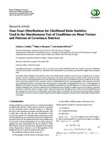
interval endpoints was negative. These are cases where the three EV models are plausible, since the value of c = 0 is included in the interval. Figure 1 shows the coverage frequencies of the quantiles of interest contained in Tables 3 to 5 in a graphical way. Figures 2 and 3 show the ratios of the lengths of the relative profile likelihood intervals under the selected EV model compared to those under the GEV model and Figures 4 and 5 give the length of profile likelihood intervals for the GEV using boxplots in which the box corresponds to the interquartile range and the whiskers have a maximum length of 1.5 times the interquartile range. Points beyond the end of the whiskers are represented individually and the line inside the box is the median. Only samples for which all intervals covered the true value of the quantile were considered in these graphs. Some remarks about the tables and figures are given below. Note that EV submodels are selected automatically, based only on the sign and size of cˆ, so the reported coverage frequencies correspond to a ‘worst case’ scenario. With a real data set, additional external information from experts would be taken into account for choosing an adequate submodel, and consequently the statistical modeling would be more efficient. 1. Coverage frequencies of GEV profile likelihood intervals and number of samples with estimation problems. Coverage frequencies of relative profile likelihood intervals for the GEV were very stable throughout the range of values of c for both quantiles. They tend to decrease as c moves towards more negative values. For n = 100 there were no numerical problems when calculating the mle’s. For n = 50 the number of samples with numerical problems was insignificant. However for n = 25, more samples presented problems in the case of Weibull models with values of c smaller than −0.2. The number of problematic cases grows as c goes to −0.5 and is above 1.8% for c = −0.4 and above 5% for c = −0.5. The number of samples that had numerical problems was the same for both quantiles considered. Therefore, numerical problems are associated to small sample sizes and Weibull models with large negative values of c. 2. Coverage frequencies of EV profile likelihood intervals. Coverage frequencies of relative profile likelihood function intervals for the EV were not so stable, and in all cases there is a region of decrease, mainly in the Fr´echet domain, where frequencies drop, as shown in Figure 1. This region grows wider as the sample size gets smaller, and the value where the minimum occurs shifts to the right from around 0.1 for n = 100 to around 0.2 for n = 25. The drop is always more pronounced for Q.99 than for Q.95 . This can be explained by the fact that for the samples that did not cover the true value of the quantile, the mle cˆ was negative in most cases and the whole interval lay below this true value and therefore underestimated it (see the second columns in Tables 3 and 4). In the Fr´echet cases, these problems were associated to estimating a large Fr´echet quantile with a Weibull model that has a bounded right tail. 3. Coverage frequencies of aml intervals. Aml intervals always had poorer coverage frequencies than relative profile likelihood intervals for the GEV for all the sample sizes considered here. Coverage frequencies for aml intervals calculated for the GEV and EV distributions are almost identical. Although coverage frequencies for these intervals improve as the sample size grows, as predicted by asymptotic theory, they 7

can be very poor for n = 25 and 50, and still unsatisfactory even for n = 100. This indicates that samples of greater size are required for these intervals to have suitable coverage frequencies. In all cases the intervals that failed to cover the true values tended to underestimate them. 4. Asymmetry of proportions of intervals that exclude the true value. Except for one single case (n = 50, Q.99 , c = 0.5) there were always more relative profile likelihood intervals that underestimated than overestimated the true value of the quantile. This asymmetry is more pronounced for smaller sample sizes, n = 25. The asymmetry also increases as c becomes smaller and is very marked in the Weibull case. This may be due to the fact that the Weibull distribution has a finite upper limit and intervals tend to increase in size with c. Therefore estimating a large quantile from a sample with cˆ > c the interval will be larger and more likely to include the true value. However, even if this asymmetry is not desirable, the asymmetry of aml intervals is certainly much more marked than the one for profile likelihood intervals. 5. Interval lengths. Almost always intervals obtained with the GEV models are larger than those obtained with EV distributions as shown in Figures 2 and 3. Only samples where both intervals included the true value of the parameter were considered. The length of the intervals tended to be alike for large values of |c|, although there is some asymmetry in this, with Fr´echet intervals being closer in length than the corresponding Weibull cases. Also, the ratio of lengths is closer to one for Q.95 than for Q.99 . For both quantiles the largest difference occurs at c = −0.05 for n = 100 and 50, and at c = −0.1 for n = 25. In Figures 2 and 3, the region where the interquartile boxes are visible (i.e. where the length differences are more important) coincides roughly with the region where there is a drop in the coverage frequencies for the EV distributions. This shows that there is a trade off between coverage and precision in the choice of a model: There is the possibility of gaining precision in the estimation but a the risk of reducing the confidence level of the interval. It is important to note that for the same quantile and sample size, the lengths of confidence intervals grow with c, as shown by Figures 4 and 5. This is to be expected since Weibull distributions are bounded above while Gumbel and Fr´echet are not. Figure 6 shows the length between the true values of Q.01 and Q.99 of the corresponding distribution, as the parameter c increases. 6. Effect of sample size on interval length. As one would expect, the length of the intervals decreases as the sample size increases, but not uniformly. Halving the sample size from n = 50 to 25 increases interval length by a factor between 1.84 to 2.65, depending on the value of c, and by a factor of 1.56 to 1.78 when decreasing from n = 100 to 50. Also, for a fixed sample size the length of intervals for Q.99 is always larger than those of Q.95 , as shown in Figure 5. 7. Coverage frequencies of GEV shape parameter c. The coverage frequencies of the profile likelihood intervals of this parameter, shown in Table 5, are stable throughout the range of values of c, with a slight decrease for the more negative values of c. The proportion of intervals that underestimate is much larger than those that overestimate 8

the true value of c, especially in the Weibull cases. This asymmetry diminishes as c takes larger positive values. 8. Asymmetry in the correct automatic selection of a model. The number of simulated samples where the estimator cˆ has the same sign as the true value of c, as the column “correct” shows in Table 5, depends on the value of c. Although the difference is not pronounced, it is always more likely for the same value of |c| that the signs coincide in a Weibull case than in the corresponding Fr´echet case. On the other hand, it is more likely that intervals in the Fr´echet case cover the origin, and therefore make plausible a Gumbel model, as the “negative” column shows in Table 5.

5

Rain Data Example

In the state of Michoac´an, M´exico, near its capital city Morelia, there is a monitoring meteorological station located at the Cointzio dam. This station is representative of rainfall patterns in this area. Yearly maxima of daily rainfall were obtained for 58 years in a period between 1940 and 2002. In this area, there is a marked rainy season from May to September. This data set will serve to illustrate the statistical modelling procedures suggested here. As a first step, the relative profile likelihood of the GEV shape parameter c shown in Figure 7(a) assigns plausibility only to positive values of c and the mle is cˆ = 0.21. therefore suggesting a Fr´echet model. Since rain data are necessarily non-negative, for physical reasons it is important to consider a Fr´echet model with a non-negative lower threshold parameter µ ≥ 0 that could very well simplify to a two parameter Fr´echet model, where µ = 0. The relative profile likelihood of µ under the three parameter Fr´echet model shown in Figure 7(b), clearly assigns a very high plausibility to the value of µ = 0, so that the data appear to support strongly a two parameter Fr´echet model. Under this model, the maximum likelihood estimates are ˆ .95 ˆ .99 βˆ σ ˆ Q Q . 36.99 4.57 70.87 101.25 Figures 8(a) and 8(b) present together, for the sake of comparison, the corresponding relative profile likelihoods of these large quantiles of interest under the two parameter Fr´echet model and also under the GEV model without any restrictions to its parameters. The GEV model without restrictions for its threshold corresponds as well to a three parameter Fr´echet model without restriction to its threshold parameter; the corresponding Fr´echet mle’s are ˆ .95 ˆ .99 βˆ µ ˆ σ ˆ Q Q . -1.55 38.57 4.76 70.64 100.44 In terms of the GEV distribution’s parameters, the mle’s are given by ˆb a ˆ cˆ 37.02 8.1 0.21 The likelihood intervals obtained for these quantiles with the GEV model are larger and imply that larger values of these quantiles are plausible. Also in these graphs, the 9

aml GEV intervals are marked and show that their right endpoints tend to coincide with the right endpoints of the profile likelihood intervals of the two Fr´echet model for these quantiles; nevertheless the left points are much smaller than the other likelihoods endpoints and therefore include small values of the quantiles that are implausible under both models (two parameter Fr´echet and the GEV). That is, the aml intervals tend to underestimate the values of the quantiles. The likelihood ratio statistic of these two models for this data set is   ˆ x LFr´echet µ = 0, σ ˆ , β;   = 0.9983. W = ˆ x LFr´echet µ ˆ, σ ˆ , β;

Since these models are nested, the observed value of −2 log W = 0.0034 has p-value of 0.9535 under the asymptotic chi-square distribution with one degree of freedom. The observed value of 0.9983 with a p-value of 0.32, indicates that the two Fr´echet parameter model makes the observed sample equally probable. However since the two Fr´echet parameter model is simpler and fits adequately the data set as shown in Figure 9(a), this model should be preferred. Figure 9(a) shows the corresponding quantile-quantile plot with pointwise likelihood bands that includes all observed values. Moreover, this model should be taken into account due to the physical considerations stated above. Likelihood-confidence intervals of 15% likelihood level and approximate 95% confidence level for the quantiles of interest Q.95 and Q.99 under the two parameter Fr´echet model are (61.6, 85.06) and (83.02, 131.66) respectively. Finally Figure 9(b) shows the return periods plot with profile likelihood 15% level bands marked for both the GEV model and the two Fr´echet model. Since rainfall levels higher than 200ml are associated with floodings of Morelia, and since a return period of a 100 years is associated to quantile Q.99 , then the probability is extremely low that the city of Morelia gets flooded within 100 years.

6

Conclusions

Overall, profile likelihood intervals of large quantiles of Extreme Value distributions and of the GEV shape parameter c performed well and had adequate coverage frequencies for moderate and small sample sizes. In contrast, the corresponding aml intervals are symmetric about the mle and had lower and poor coverage frequencies in the case of samples of size n ≤ 100. Moreover, a large proportion of the aml intervals that excluded the true value tended to underestimate it. The aml intervals are frequently used in Extreme Value Theory applications without notice of these issues. Profile likelihood intervals of EV submodels tend to be shorter than the corresponding GEV profile likelihood intervals when the true value of c is close to zero, that is when c ∈ (−.05, .05) if the sample size is n ≤ 50. Nevertheless, their coverage frequencies are adequate so that they should be preferred when the model selection of an EV is clear. However, if there is no additional external information on a given preferred EV model suggested by the theory behind the specific phenomenon of interest, then using GEV profile likelihood intervals is a conservative procedure since they also had good coverage frequencies, even though these intervals tended to be larger. 10

Profile likelihood intervals of c may serve as an aid in model selection. They also had adequate coverage frequencies. For values of c in a region around zero (−0.01, 0.01) approximately 95% of the likelihood intervals for the simulated samples included the value of zero. These are cases where the three EV models are plausible for the given sample, and also where the Gumbel model usually has a moderate or high plausibility given by the relative profile likelihood of c at zero. This is indicative of the need of additional external information of experts and other diagnostic methods to select adequately the best and most simple model for the phenomenon of interest. This will improve the estimating precision, and will prevent underestimating the quantile of interest. Finally, for sample sizes smaller than 50 and in the case that a Weibull model might be an appropriate choice, then the use of the exact likelihood function is suggested in order to make inferences about the parameters of interest through profile likelihood intervals.

7

Acknowledgments

Work partially financed by CONCYTEG, Grants 05-02-K117-027-A04 and 05-02-K117-099. The authors thank Instituto Mexicano de Tecnolog´ıa del Agua at Cuernavaca, M´exico, for facilitating the rainfall data set.

References [1] Cheng, R.C.H., Iles, T.C. Embedded models in three-parameter distributions and their estimation. JRSS B, V. 52 (1990), pp. 135-149. [2] Fisher, R. A., Tippett, L.H.C. Limiting forms of the frequency distributions of the largest or smallest member of a sample. Proceedings of the Cambridge Philosophical Society, V. 24 (1928), pp. 180-190. [3] Jenkinson, A.F. The frequency distribution of the annual maximum (or minimum) values of meteorological events. Quarterly J. Royal Meteorological Society 81 (1955), pp. 158172. [4] Kalbfleisch, J. Probability and Statistical Inference, V. 2: Statistical Inference. Springer Verlag, New York, 1985. [5] Meeker, W. O. and Escobar, L. A. Statistical Methods for Reliability Data. John Wiley & Sons, New York, 1998. [6] Montoya, J. A., D´ıaz-Franc´es, E., and Sprott, D. A. On a Criticism of the Profile Likelihood Function. Statistical Papers, in press. [7] Von Mises, R.(1954). La distribution de la plus grande de n valeurs, in Selected Papers, V. II, American Mathematical Society, Providence, RI. 1954, pp. 271-294.

11

n=100, Q95

c -0.5 -0.4 -0.3 -0.2 -0.1 -0.05 -0.01 -0.001 0.0 0.001 0.01 0.05 0.1 0.2 0.3 0.4 0.5

SUBMODEL Profile Likelihood Ints. < C. F. > < 543 9314 143 984 438 9408 154 884 442 9374 184 888 379 9449 172 872 347 9457 196 844 392 9423 185 805 400 9395 205 755 423 9374 203 778 394 9415 191 751 416 9380 204 792 443 9396 161 785 446 9358 196 735 496 9302 202 781 285 9495 220 727 280 9506 214 757 298 9477 225 782 296 9472 232 740

AML C. F. 8877 9003 9023 9076 9120 9169 9215 9191 9221 9180 9194 9240 9195 9262 9232 9214 9260

GEV

c -0.5 -0.4 -0.3 -0.2 -0.1 -0.05 0.0 0.05 0.1 0.2 0.3 0.4 0.5

< 576 552 505 433 412 447 503 567 64 461 333 309 283

C. F. 9288 9309 9345 9435 9432 9379 9327 9243 9168 9333 9458 9492 9468

> 136 139 15 132 156 174 17 19 192 206 209 199 249

< 1382 1346 1271 1195 1105 1111 1047 1067 1069 1001 978 985 993

C. F. 845 8547 8663 8763 8881 8875 8945 8927 8929 8997 9022 9015 9007

c -0.5 -0.4 -0.3 -0.2 -0.1 -0.05 0 0.05 0.1 0.2 0.3 0.4 0.5

< 757 639 599 556 547 595 586 714 734 819 625 398 353

C. F. 9107 9244 9287 9313 9315 9259 9252 9103 9109 9008 9195 9414 9434

> 136 117 114 131 138 146 162 183 157 173 18 188 213

< 2165 2037 1839 1759 1658 1659 1535 1576 1481 1457 1434 1311 1385

C. F. 755 7834 8097 8209 833 8334 8457 8421 8518 8543 8566 8689 8615

Profile Likelihood Ints. < C. F. > 543 9314 143 438 9408 154 442 9374 184 378 9450 172 344 9469 187 363 9464 173 315 9496 189 338 9469 193 325 9490 185 332 9473 195 341 9509 150 309 9501 190 321 9477 202 267 9513 220 280 9506 214 298 9477 225 296 9472 232

> 139 113 89 52 36 26 30 31 28 28 21 25 24 11 11 04 0 n=50 > < 168 572 107 551 66 505 42 433 14 383 14 388 8 351 6 346 2 359 2 304 0 297 0 307 0 283 n=25 > < 285 583 129 55 64 545 32 526 12 499 7 485 8 398 3 43 1 382 0 392 0 338 0 286 0 307

SNP 0 0 0 0 0 0 0 0 0 0 0 0 0 0 0 0 0

< 984 884 887 872 842 805 755 777 751 792 784 731 781 727 757 782 740

AML C. F. 8877 9003 9024 9076 9124 9170 9216 9192 9221 9182 9196 9245 9195 9262 9232 9214 9260

> 139 113 89 52 34 25 29 31 28 26 20 24 24 11 11 04 0

C. F. 9287 9308 9345 9435 9466 9449 9486 9466 9449 9491 9494 9494 9468

> 136 139 15 132 151 163 163 188 192 205 209 199 249

SNP 5 2 0 0 0 0 0 0 0 0 0 0 0

< 1379 1343 1271 1195 1105 1112 1045 1063 1068 1001 977 985 993

C. F. 8448 8548 8663 8763 8882 8876 8947 8931 893 8997 9023 9015 9007

> 168 107 66 42 13 12 8 6 2 2 0 0 0

C. F. 8787 9153 9264 9328 9356 9365 9439 9385 9458 9435 9482 9526 948

> 115 109 112 129 136 145 158 182 157 173 18 188 213

SNP 515 188 79 17 9 5 5 3 3 0 0 0 0

< 1826 1886 1773 1744 1648 1656 1528 1571 1478 1457 1433 1311 1385

C. F. 7469 7815 8089 8208 8331 8332 8459 8423 8518 8543 8567 8689 8615

> 19 111 59 31 12 7 8 3 1 0 0 0 0

Table 3. Coverage frequencies for Q.95 with sample sizes 100, 50 and 25. C.F. stands for Coverage Frequencies, ‘’ the number that fell above and SNP represents the number of samples with numerical problems.

12

n=100, Q99

c -0.5 -0.4 -0.3 -0.2 -0.1 -0.05 -0.01 -0.001 0.0 0.001 0.01 0.05 0.1 0.2 0.3 0.4 0.5

SUBMODEL Profile Likelihood Ints. < C. F. > < 590 9332 78 1730 448 9460 92 1376 418 9440 142 1227 401 9444 155 1128 335 9376 289 1054 353 9325 322 967 431 9286 283 913 494 9242 264 923 490 9264 246 923 510 9247 243 930 570 9223 207 907 863 8913 224 875 857 8925 218 887 282 9486 232 845 269 9496 235 857 291 9472 237 887 288 9477 235 865

AML C. F. 8258 8622 8770 8870 8940 9028 9083 9074 9077 9065 9091 9124 9113 9155 9143 9113 9135

GEV

-0.5 -0.4 -0.3 -0.2 -0.1 -0.05 0.0 0.05 0.1 0.2 0.3 0.4 0.5

628 576 521 429 555 421 624 923 1131 577 313 286 264

9306 9355 9356 9412 9177 9320 9157 8872 8661 9190 9459 9479 9461

SUBMODEL 66 2297 69 1915 123 1702 159 1475 268 1399 259 1326 219 1249 205 1261 208 1232 233 1138 228 1127 235 1172 275 1137

7690 8083 8298 8525 8598 8672 8750 8739 8768 8862 8873 8828 8863

13 623 2 575 0 521 0 429 3 399 2 383 1 361 0 348 0 333 0 289 0 281 0 286 0 264 n=25

9306 9354 9359 9452 9440 9460 9459 9455 9460 9478 9491 9479 9461

66 69 120 119 161 157 180 197 207 233 228 235 275

-0.5 -0.4 -0.3 -0.2 -0.1 -0.05 0.0 0.05 0.1 0.2 0.3 0.4 0.5

772 668 624 531 535 572 659 1015 1252 1363 788 411 326

9166 9247 9221 9290 9250 9234 9149 8790 8555 8435 8999 9357 9414

SUBMODEL 62 3069 85 2687 155 2321 179 2078 215 1916 194 1901 192 1755 195 1822 193 1639 202 1618 213 1607 232 1492 260 1593

6896 7309 7678 7922 8083 8099 8245 8178 8361 8382 8393 8508 8407

35 4 1 0 1 0 0 0 0 0 0 0 0

8893 9199 9257 9354 9349 9389 9437 9396 9431 9409 9457 9482 9442

62 64 100 113 145 148 153 183 189 202 213 232 260

> 12 2 3 2 6 5 4 3 0 5 2 1 0 0 0 0 0 n=50

Profile Likelihood Ints. < C. F. > 590 9332 78 448 9460 92 418 9440 142 401 9448 151 335 9493 172 341 9479 180 299 9490 211 330 9468 202 324 9476 200 349 9458 193 337 9485 178 293 9490 217 315 9467 218 263 9505 232 269 9496 235 291 9472 237 288 9477 235

530 549 564 516 497 458 405 418 377 389 330 286 298

< 1731 1375 1227 1128 1053 966 913 923 924 930 905 869 883 845 857 888 864

AML C. F. 8257 8623 8770 8870 8943 9031 9084 9075 9076 9069 9094 9130 9117 9155 9143 9112 9136

> 12 2 3 2 4 3 3 2 0 1 1 1 0 0 0 0 0

GEV 5 2 0 0 0 0 0 0 0 0 0 0 0

2293 1913 1702 1475 1398 1325 1249 1257 1231 1137 1127 1173 1136

7689 8083 8298 8525 8602 8675 8751 8743 8769 8863 8873 8827 8864

13 2 0 0 0 0 0 0 0 0 0 0 0

GEV 515 188 79 17 9 5 5 3 3 0 0 0 0

2600 2509 2244 2061 1907 1896 1748 1817 1636 1616 1606 1492 1593

6872 7299 7677 7922 8084 8099 8247 8180 8361 8384 8394 8508 8407

13 4 0 0 0 0 0 0 0 0 0 0 0

SNP 0 0 0 0 0 0 0 0 0 0 0 0 0 0 0 0 0

Table 4. Coverage frequencies for Q.99 with sample sizes 100, 50 and 25. C.F. stands for Coverage Frequencies, ‘’ the number that fell above and SNP represents the number of samples with numerical problems.

13

15% Profile Likelihood Intervals for c with n=100 c < Cov. Freq. > Correct Negative -0.5 564 9328 108 10000 0 -0.4 396 9479 125 10000 0 -0.3 410 9425 165 10000 45 -0.2 371 9451 178 9993 1721 -0.1 348 9465 187 9375 6988 -0.05 297 9458 245 7787 8766 -0.01 272 9490 238 5772 9416 -0.001 296 9465 239 5264 9458 0.0 303 9460 237 0 9460 0.001 309 9461 230 4735 9454 0.01 286 9483 231 5357 9392 0.05 255 9482 263 7299 8605 0.1 299 9444 257 8866 6773 0.2 244 9463 293 9902 2232 0.3 246 9465 289 9992 265 0.4 236 9483 281 10000 5 0.5 259 9467 274 10000 0 15% Profile Likelihood Intervals for c with n=50 c < Cov. Freq. > Correct Negative -0.3 467 9394 139 9989 1653 -0.2 388 9441 171 9821 5015 -0.1 371 9416 213 8515 8206 -0.05 327 9466 207 7075 8996 0.0 317 9442 241 0 9442 0.05 287 9456 257 6445 8987 0.1 321 9419 260 7939 7917 0.2 255 9460 285 9426 5022 0.3 256 9463 281 9833 2276 0.4 271 9458 271 9969 767 0.5 246 9434 320 9988 158

Table 5. Coverage frequencies for c with sample sizes 100 and 50: ‘’ the number that fell above, ‘Correct’ stands for the number of samples with correct choice of EV and ‘Negative’ stands for the number of samples with negative product of interval endpoints.

14

Coverage frequencies for Q

0.95

with n=100

Coverage frequencies for Q

0.99

1

with n=100

1

0.95

0.95

0.9

Coverage

Coverage

0.9

0.85

0.8

ProfileDVEG ProfileSub amlDVEG amlSub

0.75

0.7 −0.5

0

0.85

0.8 ProfileGEV ProfileSub amlGEV amlSub

0.75

0.7

0.65 −0.5

0.5

0

c

c

(a)

(b)

Coverage frequencies for Q0.95 with n=50

0.5

Coverage frequencies for Q0.99 with n=50

1

1

0.95

0.95

0.9

Coverage

Coverage

0.9

0.85

0.85

0.8

0.8 ProfileGEV ProfileSub amlGEV amlSub

0.75

0.7 −0.5

0

ProfileGEV ProfileSub amlGEV amlSub

0.75

0.7

0.65 −0.5

0.5

0

c

c

(c)

(d)

Coverage frequencies for Q0.95 with n=25

0.5

Coverage frequencies for Q0.99 with n=25

1

1

0.95

0.95

0.9

Coverage

Coverage

0.9

0.85

0.8

ProfileGEV ProfileSub amlGEV amlSub

0.75

0.7 −0.5

0

0.85

0.8

0.75

ProfileGEV ProfileSub amlGEV amlSub

0.7

0.65 −0.5

0.5

0

c

c

(e)

(f)

0.5

Figure 1: Coverage frequencies. The left column corresponds to Q95 , the right to Q99 . The first row corresponds to a sample size of 100, the middle row to sample size 50 and the bottom row to sample size 25. 15

Ratios of interval lengths for Q0.95 with n=100 1 0.9 0.8

Ratio

0.7 0.6 0.5 0.4 0.3 0.2 0.1 0

−0.5 −0.4 −0.3 −0.2 −0.1 −0.05 −0.01−0.001

0

0.001 0.01 0.05

0.1

0.2

0.3

0.4

0.5

0.2

0.3

0.4

0.5

c Ratios of interval lengths for Q

0.99

with n=100

1.2

1

Ratio

0.8

0.6

0.4

0.2

0 −0.5 −0.4 −0.3 −0.2 −0.1 −0.05 −0.01−0.001

0

0.001 0.01 0.05

0.1

c

Figure 2: Ratio of length of likelihood-confidence intervals for Q95 (top) and Q99 (bottom) for the submodel over length of intervals for the GEV, sample size 100.

16

Ratios of interval lengths for Q0.95 with n=50

Ratios of interval lengths for Q0.99 with n=50

1.4

1.3

1.3

1.2

1.2

1.1

1.1

1

1

0.9 0.8

0.8

Ratio

Ratio

0.9

0.7 0.6

0.7 0.6 0.5

0.5

0.4

0.4 0.3

0.3

0.2

0.2

0.1

0.1

0

−0.5 −0.4 −0.3 −0.2 −0.1 −0.05

0

0.05 0.1

0.2

0.3

0.4

0

0.5

(a)

(b)

Ratios of interval lengths for Q0.95 with n=25

0.05 0.1

0.2

0.3

0.4

0.5

0.4

0.5

Ratios of interval lengths for Q0.99 with n=25 1.3

1.3

1.2

1.2

1.1

1.1

1

1

0.9

0.9

0.8

0.8

Ratio

Ratio

0

c

1.4

0.7 0.6

0.7 0.6 0.5

0.5

0.4

0.4 0.3

0.3

0.2

0.2

0.1

0.1

0

−0.5 −0.4 −0.3 −0.2 −0.1 −0.05

c

−0.5 −0.4 −0.3 −0.2 −0.1 −0.05

0

0.05 0.1

0.2

0.3

0.4

0

0.5

−0.5 −0.4 −0.3 −0.2 −0.1 −0.05

0

c

c

(c)

(d)

0.05 0.1

0.2

0.3

Figure 3: Ratio of length of likelihood-confidence intervals for Q95 (left) and Q99 (right) for the submodel over length of intervals for the GEV, sample sizes 50 (top) and 25 (bottom).

17

Lengths of profile likelihood intervals for Q0.95 with n=100 20 18 16 14

Length

12 10 8 6 4 2 0 −0.5 −0.4 −0.3 −0.2 −0.1 −0.05−0.01−0.001 0 0.001 0.01 0.05 0.1 c Lengths of profile likelihood intervals for Q

0.99

0.2

0.3

0.4

0.5

0.3

0.4

0.5

with n=100

120

100

Length

80

60

40

20

0 −0.5 −0.4 −0.3 −0.2 −0.1 −0.05−0.01−0.001 0 0.001 0.01 0.05 0.1 c

0.2

Figure 4: Length of profile likelihood-confidence intervals for Q95 (top) and Q99 (bottom) for the GEV, sample size 100.

18

Lengths of profile likelihood intervals for Q0.95 with n=50

Lengths of profile likelihood intervals for Q0.99 with n=50

700

60

600

50

500 Length

Length

40

30

400 300

20

200

10

100 0

0 −0.5 −0.4 −0.3 −0.2 −0.1 −0.05

0 c

0.05 0.1

0.2

0.3

0.4

0.5

−0.5 −0.4 −0.3 −0.2 −0.1 −0.05

(a)

0.05 0.1

0.2

0.3

0.4

0.5

(b)

Lengths of profile likelihood intervals for Q0.95 with n=25

Lengths of profile likelihood intervals for Q0.99 with n=25

2000

20000

1800

18000

1600

16000

1400

14000

1200

12000 Length

Length

0 c

1000 800

10000 8000

600

6000

400

4000

200

2000

0

0 −0.5 −0.4 −0.3 −0.2 −0.1 −0.05

0 c

0.05 0.1

0.2

0.3

0.4

0.5

−0.5 −0.4 −0.3 −0.2 −0.1 −0.05

(c)

0 c

0.05 0.1

0.2

0.3

0.4

0.5

(d)

Figure 5: Length of profile likelihood-confidence intervals for Q95 (left) and Q99 (right), sample sizes n = 50 (top) and n = 25 (bottom) for the GEV. One outlying sample was excluded from plots (c) and (d).

19

Difference between Q

.99

and Q

.01

for the GEV

20 18 16

Difference

14 12 10 8 6 4 −0.5

0 c

0.5

1

1

0.9

0.9

0.8

0.8

0.7

0.7

0.6

0.6 Rp(µ)

Rp(c)

Figure 6: Difference between Q01 and Q99 for the GEV models with a = b = 1 and corresponding values of c.

0.5

0.5

0.4

0.4

0.3

0.3

0.2

0.2

0.1

0.1

0 −0.4

−0.2

0

0.2

0.4

0.6

0.8

0 −450

1

c

(a)

−400

−350

−300

−250

−200 µ

−150

−100

−50

0

50

(b)

Figure 7: Rain data example: (a) Relative profile likelihood of GEV shape parameter c. (b) Relative profile likelihood of threshold parameter in three parameter Fr´echet model.

20

1

1 Frechet µ=0 GEV

0.8

0.8

0.7

0.7

0.6

0.6

0.5

0.5

0.4

0.4

0.3

0.3

0.2

0.2

0.1

0.1

0 50

100 Q.95

Frechet µ=0 GEV

0.9

Rp(Q.99)

Rp(Q.95)

0.9

0 50

150

100

150

200

250

300

Q.99

(a)

(b)

Figure 8: Rain data example: Relative profile likelihood of (a) Q.95 , (b) Q.99 .

140 400

120

350

Delta GEV Profile GEV Profile Fréchet µ=0

300 Return level in mm

Orderated data

100

80

250

200

150

60

100

40 50

20 20

30

40

50

60 70 80 Estimated quantiles

90

100

0 0 10

110

1

2

10

10

3

10

Return period in years

(a)

(b)

Figure 9: Rain data example: (a) Q-Q plot for the two parameter Fr´echet model. (b) Return period plot.

21