Profiling and Tracing in Linux Sameer Shende Department of Computer and Information Science University of Oregon, Eugene, OR, USA
[email protected]
Abstract Profiling and tracing tools can help make application parallelization more effective and identify performance bottlenecks. Profiling presents summary statistics of performance metrics while tracing highlights the temporal aspect of performance variations, showing when and where in the code performance is achieved. A complex challenge is the mapping of performance data gathered during execution to high-level parallel language constructs in the application source code. Presenting performance data in a meaningful way to the user is equally important. This paper presents a brief overview of profiling and tracing tools in the context of Linux - the operating system most commonly used to build clusters of workstations for high performance computing.
1. Introduction Understanding the behavior of parallel programs is a daunting task. Two activities that aid the user in understanding the performance characteristics of his/her program are profiling and tracing. To understand the behavior of the parallel program, we must first make its behavior observable. To do this, we regard the execution of a program as a sequence of actions, each representing some significant activity such as the entry into a routine, the execution of a line of code, a message communication or a barrier synchronization. These actions become observable when they are recorded as events. Thus, an event is an encoded instance of an action [10]. It is the fundamental unit we use in understanding the behavior of a program. More specifically the execution of an event interrupts the program and initiates one of the following responses: • the computation is stopped • visible attributes of the event are recorded, or • statistics are collected. After an event response is completed, control returns to the program. The response to an event depends on its use: debugging; tracing; or profiling. Profiling updates summary statistics of execution when an event occurs. It uses the occurrence of an event to keep track of statistics of performance metrics. These statistics are maintained at runtime as the process exe-
cutes and are stored in profile data files when the program terminates. Profiles are subsequently analyzed to present the user with aggregate summaries of the metrics. Tracing, on the other hand, records a detailed log of timestamped events and their attributes. It reveals the temporal aspect of the execution. This allows the user to see when and where routine transitions, communication and user defined events take place. Thus, it helps in understanding the behavior of the parallel program. Performance analysis based on profiling and tracing involves three phases: • instrumentation or modification of the program to generate performance data, • measurement of interesting aspects of execution which generates the performance data and • analysis of the performance data.
2. Instrumentation Common to both profiling and tracing is the instrumentation phase where instructions are added to the program to generate performance data. Instrumentation helps in identifying the section of code that is executing when an event is triggered. It is also responsible, during execution, for measuring the resources consumed and mapping these resources to program entities, such as routines and statements. Relating the code segments
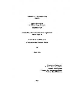
back to source-code constructs and entities that the user can comprehend is important. As shown in Figure 1., instrumentation can be added to the program at any stage during the compilation/execution process from user-added calls in the source code to a completely automated approach. (Events are triggered by the execution of the instrumentation instructions at runtime.) Moving down the stages from source code instrumentation to runtime instrumentation, the instrumentation mechanism changes from language specific to platform specific. Making an instrumentation API specific to a language for source code instrumentation may make the instrumentation portable across multiple compilers and platforms that support the language. However, the instrumentation may not work with other languages. Targeting the instrumentation at the executable level ensures that applications written in any language that generates an executable would benefit from the instrumentation on the specific platform. However, it is more difficult to map performance data back to source-code entities, especially if the application’s highlevel programming language (such as HPF or ZPL), is translated to an intermediate language (such as Fortran or C) during compilation. There is often a trade-off between what level of abstraction the tool can provide and how easily the instrumentation can be added. The JEWEL [19] package requires that calls be added manually to the source code. While providing flexibility, the process can be cumbersome and time consuming. A preprocessor can generate instrumented source code by automatically inserting annotations into the original source. This approach is taken by SvPablo [14] and AIMS [20] for C and Fortran, and by TAU [15] with PDT for C++ [18]. Instrumentation can be added by a compiler as in gprof [5] (with the -pg commandline switch for the GNU compilers). Instrumentation can also be added during linking when the executable image is created by linking multiple object files and libraries together. Packages that use this method include VampirTrace [13], and PICL [12] for MPI and PVM message passing libraries. When an inter-process communication call is executed, the instrumented library acts as a wrapper that calls the profiling and tracing routines before and after calling the corresponding uninstrumented library call. This is achieved by weak library bindings. However, often program sources and libraries are unavailable to the users and it is necessary to examine the performance of executable images. Pixie [16] and Atom [17] are tools that rewrite binary executable files while adding the instrumentation, but are not currently available under Linux.
Language specific
Source code
TAU, Jewel
Preprocessor
TAU/PDT, AIMS, SvPablo
Source code
Compiler
gprof
Object code
Libraries
Linker
Executable Platform specific
VampirTrace, PICL Atom, Pixie Paradyne
Execution
Figure 1: Instrumentation options range from language specific to platform specific mechanisms. All these approaches require the programer to modify the application, re-compile and re-execute the instrumented application to produce the performance data. Sometimes, re-execution of an application using the performance analysis tool is not a viable alternative while searching for performance bottlenecks. This is true for long-running tasks such as database servers. Paradyne [9] automates the search for bottlenecks in an application at runtime by selectively inserting and deleting instrumentation using the DynInst [7] dynamic instrumentation package. After instrumentation, we execute the program and perform measurements, in the form of profiling and tracing and analyze the data.
3. Profiling Profiling shows the summary statistics of performance metrics that characterize the performance of an application. Examples of metrics include: the CPU time associated with a routine; the count of the secondary data cache misses associated with a group of statements; the number of times a routine executes; etc. These metrics are typically presented as sorted lists that show the contribution of the routines. Two main approaches to profil-
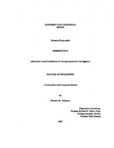
ing include sampled process timing and measured process timing. In profiling based on sampling, a hardware interval timer periodically interrupts the execution. Instead of time, these interrupts could be triggered by CPU performance counters, that measure events in hardware, as well. Commonly employed tools such as prof [4] and gprof [5] use time based sampling. When an interrupt occurs, the state of the program counter (PC) is sampled and a histogram that represents the frequency distribution of PC samples is maintained. The program’s image file and symbol table are used post-mortem to calculate the time spent in each routine as the number of samples in a routine’s code range times the sampling period. Instead of the PC, the callstack of routines can be sampled too. In this case, a table that maintains the time spent exclusively and inclusively (of called child routines) for each routine, is updated, when an interrupt occurs. Then, the exclusive time of the currently executing routine and the inclusive time of the other routines that are on the callstack are incremented by the interinterrupt time interval. Additionally, in gprof, each time a parent calls a child function, a counter for that parentchild pair is incremented. Gprof then shows the sorted list of functions and their call-graph descendents. Below each function entry are its call-graph descendents, showing how their times are propagated to it. In profiling based on measured process timing, the instrumentation is triggered at routine entry and exit. At these points, a precise timestamp is recorded and performance metrics comprising of timers and counters are updated. TAU [15] uses this approach. TAU’s modular profiling and tracing toolkit features support for hardware performance counters, selectively profiling groups of functions and statements, user-defined events and threads. It works with C++, C and Fortran on a variety of platforms including Linux. Its modules can be assembled by the user during the configuration phase and a profiling or tracing library can be tailor-made to the user’s specification. Profiles can be analyzed using racy, a GUI, as shown in Figure 2. or pprof, a prof-like utility that can sort and display tables of metrics in text form.
3.1 Hardware Performance Counters A profiling system needs access to an accurate and a high-resolution clock. The Intel Pentium(R) family of processors contains a free-running 64-bit time-stamp counter which increments once every clock cycle. This is accessible as Model Specific Registers built into the processor to profile hardware performance. These registers can also be used to monitor hardware performance
Figure 2: TAU’s profile browser tool racy counters that record counts of processor specific events such as memory references, cache misses, floating point operations and bus activity. The Intel PentiumPro(R) and Pentium II(R) CPUs have two performance counters available as 32-bit registers that can count at most 66 different events (two at a time). Tools such as pperf [6] and PCL [1] provide access to these registers under the Linux operating system. PCL provides a uniform API, in the form of a library, to access the hardware performance counters on a number of platforms. Under Linux, the counters are not saved on each context switch operation and PCL recommends performing measurements on a lightly loaded system. PerfAPI [2] is another project that will provide a uniform API for accessing hardware performance counters on different platforms, including Linux. Profiling can present the total resources consumed by program level entities. It can show the relative contribution of the routines to the profile of the application and can provide insight in locating performance hotspots.
4. Tracing Typically, profiling shows the distribution of execution time across routines. It can show the code locations associated with specific bottlenecks, but it does not show the temporal aspect of performance variations. The advantage of profiling is that statistics can be maintained during execution and it requires a small amount of storage. Tracing the execution of a parallel program shows when an event occurred and where it occurred, in terms of the location in the source code and the process that executed it. An event is typically represented by an ordered tuple that consists of the event identifier, the timestamp when the event occurred, where it occurred (the location may be specified by the node and thread identifiers) and an optional field of event specific information. In addition to the event-trace, a table that maps
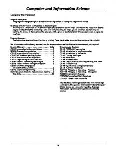
Figure 3: Vampir displays TAU traces from a multi-threaded SMARTS application written in C++ the event identifier to an event name and its characteristics is also maintained. Tracing involves storing data associated with an event in a buffer and periodically writing the buffer to stable storage. This involves event logging, timestamping, trace buffer allocation and trace output. The traces can be merged subsequently and corrected for perturbation [10] that may have been caused due to the overhead introduced by the instrumentation. Finally, visualization and analysis of event-traces helps the user understand the behavior of the parallel program.
4.1 Clock Synchronization Tracing a program that executes on a cluster of workstations requires access to an accurate and a globally synchronized real-time clock to order the events accurately with respect to a global time base. Clock synchronization can be implemented in hardware, as in shared memory multiprocessors. It can also be achieved by using software protocols such as the Network Time Protocol [11] which synchronizes the clocks to a within a few milliseconds on a LAN or a WAN, or it can be implemented within the tool environment as in BRISK [19]. For greater accuracy, a GPS satellite receiver may be used to synchronize the system clock accurately to within a few microseconds as described in [8]. Profiling does not require a globally synchronized real-time clock
but tracing does.
5. Performance Analysis and Visualization Parallel programs produce vast quantities of multidimensional data. Representing this data without overwhelming the user with unnecessary detail is critical to the tools’ success. It can be represented effectively using a variety of visualization techniques [14] such as scatter plots, Kiviat diagrams, histograms, Gantt charts, interaction matrices, pie charts, execution graphs and tree displays. ParaGraph [3] is a trace visualization tool that incorporates the above techniques and has inspired performance views in several other tools. It is available under Linux and works with PICL traces. It contains a rich set of visualizations and is extensible by the user. Vampir [13] is a robust, commercial trace visualization tool available under Linux. Figure 3. is a Vampir display of traces generated by TAU. It shows a space-time diagram that highlights when events such as routine transitions take place on different processors. Pablo [14] provides a user directed-analysis of performance data visualization by providing a set of performance data transformation modules that are interconnected graphically to create an acyclic data analysis graph. Performance data flows through this graph and metrics can be
computed by different user-defined modules.
6. Conclusion This paper presented a brief overview of some profiling and tracing tools that are available under Linux, and the techniques that they use for instrumentation, measurement and visualization. Linux is increasingly used by the scientific community for parallel simulations on clusters of personal computers. With growing complexity of component based, high performance scientific frameworks [18] , tools often encounter a “semanticgap”. They present performance information that is too low level and does not relate well with source code constructs in the high-level parallel languages used to program these clusters. Unless tools can present performance data in ways that are meaningful to the user, and are consistent with the user’s mental model of abstractions, their success will be limited.
7. Acknowledgments This work was supported by the U.S. Government, Department of Energy DOE2000 program #DEFC0398ER259986.
References [1]R. Berrendorf, H. Ziegler, “PCL - The Performance Counter Library. A Common Interface to Access Hardware Performance Counters on Microprocessors”, Technical Report, FZJ-ZAM-IB-9816, Central Institute for Applied Mathematics, Research Centre Juelich GmbH, Oct 1998. URL:http://www.fz-juelich.de/zam/PT/ ReDec/SoftTools/PCL/PCL.html [2]S. Browne, G. Ho, P. Mucci, C. Kerr, “Standard API for Accessing Hardware Performance Counters”, Poster, SIGMETRICS Symposium on Parallel and Distributed Tools 1998. URL:http://icl.cs.utk.edu/projects/papi/. [3]M. Heath, J. Ethridge, “Visualizing the performance of parallel programs,” IEEE Software, Vol. 8, No. 5, 1991. URL:http://www.ncsa.uiuc.edu/Apps/MCS/ParaGraph/ParaGraph.htmls [4]S. Graham, P. Jessler, M. McKusick, “An Execution Profiler for Modular Programs”, Software - Practice and Experience, Vol. 13, pp. 671-685, 1983. [5]S. Graham, P. Kessler, M. McKusick, “gprof: A Call Graph Execution Profiler”, Proceedings of SIGPLAN ‘82 Symposium on Compiler Construction, SIGPLAN Notices, Vol. 17, No. 6, pp. 120-126, June 1982. [6]M. Goda, “Performance Monitoring for the Pentium and Pentium Pro Under the Linux Operating System”,1999.URL:http://qso.lanl.gov/~mpg/perfmon.html [7]J. Hollingsworth, B. Buck, “DyninstAPI Programmer’s Guide”, 1998. URL:http://www.cs.umd.edu/
projects/dyninstAPI/ [8]J. Hollingsworth, B. Miller, “Instrumentation and Measurement”, in The Grid: Blueprint for a New Computing Infrastructure I. Foster and C. Kesselman (Eds.), Morgan Kaufmann Publishers, San Francisco, pp.339365, 1999 [9]B. Miller, M. Callaghan, J. Cargille, J. Hollingsworth, R. Irvin, K. Karavanic, K. Kunchithapadam and T. Newhall. IEEE Computer 28(11), pp.37-46 (November 1995).URL:http://www.cs.wisc.edu/~paradyn [10]A. D. Malony, “Performance Observability”, Ph.D. Thesis, University of Illinois, Urbana, Also available as CSRD Report No. 1034, Sept. 1990. [11]Network Time Protocol, 1999. URL:http:// www.eecis.udel.edu/~ntp/ [12]Oak Ridge National Laboratory, “Portable Instrumented Communication Library”,1999. URL:http:// www.epm.ornl.gov/picl [13]Pallas GmbH, “Vampir - Visualization and Analysis of MPI Resources”, 1999. URL: http://www.pallas.de/ vampir.html [14]D. Reed and R. Ribler, “Performance Analysis and Visualization”, in The Grid: Blueprint for a New Computing Infrastructure I. Foster and C. Kesselman (Eds.), Morgan Kaufmann Publishers, San Francisco, pp.367393, 1999.URL:http://www-pablo.cs.uiuc.edu/ [15]S. Shende, A. D. Malony, J. Cuny, K. Lindlan, P. Beckman, and S. Karmesin, “Portable Profiling and Tracing for Parallel Scientific Applications using C++”, Proceedings of the SIGMETRICS Symposium on Parallel and Distributed Tools, pp. 134-145, ACM, Aug. 1998. URL:http://www.acl.lanl.gov/tau [16]Silicon Graphics Inc. Speedshop User’s Guide, 1999.URL:http://techpubs.sgi.com [17]A. Srivastava, A. Eustace, “Atom: A system for building customized program analysis tools,” In SIGPLAN Conf. on Programming Language Design and Implementation, pp. 196-205, ACM, 1994.URL:http:// www.research.digital.com/wrl/projects/om/om.html [18]The Staff, Advanced Computing Laboratory, Los Alamos National Laboratory, “Taming Complexity in High-Performance Computing” White paper, Aug 1998. Available from URL:http://www.acl.lanl.gov/software. [19]A. Waheed, D. Rover, M. Mutka, H. Smith, and A. Bakic, “Modeling, Evaluation and Adaptive Control of an Instrumentation System”, Proceedings of IEEE RealTime Technology and Applications Symposium (RTAS ‘97), pp. 100-110, June 1997.URL:http:// www.egr.msu.edu/Pgrt/ [20]J. Yan, “Performance Tuning with AIMS - An automated Instrumentation and Monitoring System for Multicomputers”, Proc. 27th Hawaii Intl. Conf. on System Sciences, Hawaii, Jan. 1994.URL:http://science.nas.nasa.gov/Groups/Tools/Projects/AIMS/