Programming Model and Low-level Language for a Coarse-Grained Reconfigurable Multimedia Processor Wim Vanderbauwhede
Martin Margala, Sai Rahul Chalamalasetti, Sohan Purohit
Dept. of Computing Science University of Glasgow, UK Email:
[email protected]
Dept. of Electrical and Computer Engineering University of Massachusetts at Lowell, Lowell, MA, USA Email:
[email protected]
Abstract— We present the architecture and programming model for MORA, a coarse-grained reconfigurable processor aimed at multimedia applications. The MORA architecure is a MIMD machine consisting of a 2-D array of reconfigurable cells (RC) with a flexible reconfigurable interconnect network. MORA is designed to support high-throughput data-parallel pipelined processing. We describe the design and implementation of the RC and present simulation results. Apart from its performance, the distinguishing feature of MORA is its design support for programmability. We present a novel assembly language, MORA assembly, which provides a low-level but flexible programming model for the architecture. Keywords: Coarse-grained Reconfigurable Processor, Multimedia Processing, Assembly Language
1. Introduction Reconfigurable architecture platforms are gaining increasing popularity as flexible, low-cost solutions for variety of modern media processing applications. In recent times, these architectures have played a major role in bridging the gap between general purpose processors and application specific circuits. With the continuously expanding domain of applications and algorithms to support, it becomes imperative that these reconfigurable processors provide a high degree of flexibility and adaptability, while at the same time being extremely cost-efficient. This has prompted more focused research on Coarse Grained Reconfigurable Architectures (CGRA), in recent times. Using the terminology of [14], MORA (Multimedia Oriented Reconfigurable Array, [5], [3], [4]) is an Array of Functional Units, as opposed to Hybrid Architectures (which are typically using a combination of an ordinary processor with a reconfigurable fabric, e.g. [10], [7]) and Arrays of Processors (where the reconfigurable fabric consists of fully-feature processors, e.g. [1], [11]). Within its category, MORA bears most similarity to MATRIX [6] and Silicon Hive [2], as it shares with both architectures the in-memory processing model, i.e. every functional unit has its own local memory. However, MORA’s processing element is considerably more powerful than MATRIX’s, though considerably less complex than Silicon Hive’s. As remarked by [14], the programming techniques for architectures similar to MORA still rely on low-level languages which are relatively close to describing the corresponding hardware, i.e. assembly languages. Where
a high-level language front-end is provided (e.g. XPP [8]), the compilers cannot match the performance of the lowlevel implementations. To address this issue, the MORA architecture and instruction set has been designed to support an assembly language with a high level of flexibility and expressiveness. On the one hand, the MORA assembly language provides an easier target for high-level language compilers; on the other hand, its features greatly reduce the burden of application development in a low-level language. Amongst the key features of the MORA language are: typed operations and operands, support for vector operations through the type system, hierarchical composition of functional blocks and a powerful instruction generation and templating system. The MORA processor incorporates a Design for Programmability approach to combine ease of programming with high performance and efficient resource utilisation. Listed below are MORA’s primary objectives: 1) To provide a customisable array of reconfigurable cells enabling flexible mapping of multimedia applications. 2) To provide a stand-alone computing system. MORA reconfigurable cells control the execution flow control without requiring an auxiliary general purpose processor. 3) To provide each reconfigurable cell with sufficient amount of data and instruction memory to support unique digital signal processing capabilities owing to greater memory bandwidth, lower memory access delay and lower power. 4) To provide a flexible interconnection network so that all mapped algorithms can always operate at maximum clock speed. 5) In conjunction with the compiler software, provide a heterogeneous distribution of each operation over a proper number of reconfigurable cells, thereby allowing each cell to perform tasks independently, and at the same time obtain maximum resource utilisation.
2. Architecture The MORA architecture (Fig. 1) can loosely be compared to an island-style FPGA architecture where the Configurable Logic Blocks (CLBs) are replaced by a small DSP-style processor, the Reconfigurable Cell (RC). The architecture consists of a 2-D array of identical
Reconfigurable Cells arranged in 4 × 4 quadrants and connected through a hierarchical reconfigurable interconnection network. MORA does not include a centralised RAM system. Instead storage for data is partitioned among RCs by providing each RC with internal data memory. Each individual RC is a tiny Processor-in-Memory (PIM). This approach allows computations to be performed close to memory, thereby reducing memory access time and power hungry interactions between logic elements and data memory. It also provides for high memory access bandwidth needed to efficiently support massively parallel computations required in multimedia applications while maintaining generality and scalability of the system.
Fig. 2 MORA R ECONFIGURABLE C ELL (RC)
to have maximum possible functionality, it is necessary that the PE be modified to include signed arithmetic, logic, shifting and comparison operations.
Fig. 1 MORA ARCHITECTURE
The external data exchange is managed by a central I/O Data Controller which can access the internal memory of the RCs through standard memory interface instructions. Internal data flow is controlled in a distributed manner through a handshaking mechanism between the RCs. Each RC (Fig. 2) consists of a Processing Element (PE) for 8-bit arithmetic and logical operations, 256B dualport SRAM (data memory), and a Control Unit (CU) with a small instruction memory. The PE forms the main computational unit of the RC; the control unit synchronises the instruction queue within the RC and also controls intercell communication, allowing each RC to work with a certain degree of independence. The architectures of the PE and CU are discussed in the following sub-sections.
2.1 Processing Element The Processing Element is the main computational unit of the RC. Prior work on the design of data paths, focused on optimising the data path design and organisation for efficient single cycle arithmetic operations [9]. For the RC
Fig. 3 B LOCK DIAGRAM OF THE MORA PE
Fig. 3 shows the organisation of the modified PE. It includes the signed arithmetic data path [9] along with additional blocks for shifting and comparison operations. The logic block performs logical AND/NAND, OR/NOR, XOR/XNOR on the 8 bit operands A and B. The PE uses a logarithmic shifter to implement bitwise shifting operations on the operands. The shifter block working in conjunction with the logic block provides support for round shifting and shift out operations. Multiplexer switches use control vectors S [13:0] to route operands through the PE. The arithmetic data path is organised to provide singlecycle addition, subtraction and multiplication operations. The PE also provides two sets of registers at the input and output to enable accumulation style operations, as often required for media processing applications. Output is available at the registers every clock cycle.
2.2 Control Unit and Address Generator The control unit provides the handshaking signals between memory and data path, and ensures that the
two units work in perfect sync with each other. The unit consists of a 16-word instruction memory, three address generators, instruction decoders and instruction counters. The instruction word is 92 bits wide and encodes the operation, bases addresses for an instruction operands and output data set and address offsets for traversing through memory, as well as the number of times a specific operation is to be performed. The overall flow of the control unit is as shown in Fig. 4.
Fig. 5 MORA ADDRESS GENERATOR
Fig. 4 MORA CONTROL UNIT FLOW CHART
The address generator is shown in Fig. 5. It accepts four data fields: Base address, Step, Skip and Subset. The base address is initially loaded into the address generator, and depending on the values of Step, Skip and Subset, the address of the next memory location to fetch the data is calculated. The three fields allow the controller to move anywhere throughout the available data memory. The address generation algorithm can be written as follows: address=base_address if nops>1 tsubset=subset for 1..nops tsubset-=1 if tsubset==0 address+=skip tsubset=subset else address+=step end end end
The address generator thus generates the range of addresses on which a given instruction is to be performed. This is a key feature for media processing applications which frequently involve operations on matrices and vectors of data.
2.3 Implementation The RC provides an instruction set of 29 instructions which include arithmetic, logic, memory-based and
branching instructions. Further combined with the instruction word support for multiple execution of single instructions, the RC effectively covers the entire range of instructions required for the target application domain, thereby making it a small self contained DSP style processor. The RC functionality was verified using HDL coding, and an ASIC implementation was designed using the IBM 0.13µm CMOS process. The ASIC implementation provides single-cycle instruction execution and memory write-back, supporting a maximum operating frequency of 167MHz and power consumption of 2mW. A total transistor budget of under 100,000 transistors per RC, with competitive speed and power in the low milliwatts makes MORA a low cost, attractive solution compared to competing architectures (e.g. [1]) that employ more than three orders of magnitude extra resources .
3. Programming Model 3.1 Characteristics of the MORA processor As a coarse-grained reconfigurable architecture, the MORA processor positions itself somewhere between conventional DSPs and FPGAs. The RC is a low-complexity 8-bit DSP core with a Harvard architecture and the interconnect network is similar to that used in FPGAs. However, the RC is a processorin-memory (PIM) designed for pipelined operations on streaming data. MORA operates by transferring data in a pipeline between operations, reducing the need for write-back to memory. As a consequence the RC has no registers: all operations are performed directly on the memory addresses. Another distinct feature of the RC is the address generator which provides support for SIMD-style vector operations, i.e. performing an operation on a range of addresses. This feature is essential for efficient processing of vectors and matrices as used e.g. in image compression algorithms. Finally, MORA RCs operates asynchronously, using a simple handshake mechanism to notify downstream RCs of availability of data. Synchronous operation of all RCs
would require that at every moment every RC would execute the same number of clock cycles for an operation and that the clocks would need to be synchronised over a very large area. Having to fulfil both requirements would be extremely unpractical and inefficient.
modified memory. Using X ⇒ Y to mean “X implies Y ” or “if X then Y ”, we can define the memory update as: (a, v) ∈ M ⇒ a ∈ A (as , vs ) ∈ S ⇒ as ∈ As A00 = A \ (A ∩ As )
3.2 Processing model The RCs can receive data via two input ports A, B and transfer processed data via two output ports YL, YR. Each of these output ports can be connected to up to two RCs. The RC has two states: waiting and processing; these states depend on the state of the RC’s local memory and the states of the memories of the RCs connected to its output ports. The RC memory has two states: ready and not ready. The local memory is ready when it has received a “ready” signal from all RCs connected to its input ports (unconnected input ports are always ready). The RC will process data if its local memory is ready and all of the memories of the connected RCs are not ready (unconnected output ports are always not ready).
a00 ∈ A00 , (a00 , v00 ) ∈ M ⇒ (a00 , v00 ) ∈ M 00 M 0 = S ∪ M 00
In words, the locations in the modified subset are merged with the locations in the original memory that do not overlap with those in the modified subset. The completion of this process is indicated by the RC c setting the memory state s of all RCs in C to ready and its own memory state to not ready, i.e. sA = 0 ∧ sB = 0 and thus σ = 0 or the RC is waiting for data. The operation sequence is thus: cij = (Mi , 1, pi ,Ci )
We can formalise data processing in MORA using following notation: we define a reconfigurable cell i in state j as cij = (Mij , σij , pi ,Ci )
Denoting the signals for the local memory as sA ,sB and the signals indicating the state of the connected memories as sL1 , sL2 ,sR1 ,sR2 , we can define the state of the RC as: σ = (sA ∧ sB ) ∧ ¬(sL1 ∨ sL2 ∨ sR1 ∨ sR2 )
⇒ cij+1 = (Mi0 , 0, pi ,Ci ) ∀ck ∈ Ci : ckj = (Mk , 0, pk ,Ck ) ⇒ ckj+1 = (Mk0 , σkj+1 , pk ,Ck ) ckj+1 = (Mk0 , σkj+1 , pk ,Ck ) ∧ ∀clj+1 ⇒ ckj+2 = (Mk , 1, pk ,Ck )
(1)
with M the local memory, σ the state, p the program run by the PE and C the set of RCs connected to the outputs of c. This set is determined at design time and is static (no run-time reconfiguration). A MORA processor P with a given configuration of N reconfigurable cells can be described as P = {ci , ..., cN }.
(2)
where σ = 1 means processing and obviously σ j+1 = ¬σ j , i.e. the RC alternates between processing and waiting. Borrowing the type notation from Haskell or ML, we can define the program p as a function which takes the local memory as input and produces modified subsets of the memories in c and C: p(M) = (S, SL1 , SL2 , SR1 , SR2 ) where S indicates the modified subset. The type of p is Prog = Mem → (Mem, ..., Mem). Here Mem is the type of the memory M, defined as Mem = [(Address,Value)] (i.e. Mem is a list of address-value pairs). We can regard this type as describing all the defined values in the memory, i.e. initial values written to the memory at boot time and values resulting from processing. The definition of p is not sufficient to describe the behaviour of the RC: we need to define how the modified subsets are merged with the original memory content. Let the list of all addresses of defined memory locations, A, be denoted by the type Addresses = [Address]. Let M be the original memory, S the modified subset and M 0 the
(3)
(4) (5) ∈ Ck : σl
j+1
=0 (6)
Equations (??) and (5) show the result of running the program pi in ci on ci and all RCs in Ci ; equation (6) shows that every ck in Ci will start processing if every RC in Ck is waiting.
4. The MORA assembly language The MORA “assembly” language consists of three components: a coordination component which allows to express the interconnection of the RCs in a hierarchical fashion, an expression component which corresponds to the conventional assembly languages for microprocessors and DSPs and a generation component which allows compile-time generation of coordination and expression instances.
4.1 Expression language The MORA expression language is an imperative language with a very regular syntax similar to other assembly languages: every line contains an instruction which consists of an operator followed by list of operands. The main differences are: •
•
•
Typed operators: the type indicates the wordsize on which the operations is performed, e.g. bit, nybble, byte, short, long (resp. B, N, C, S, L) Typed operands: operands are actually tuples indicating not only the address space but also the data type, i.e. word, row, column, or matrix, and the scan direction (forward or reverse) Virtual registers and address banks: MORA has no directly accessible registers. Operations take the
•
RAM addresses as operands; however, “virtual” registers indicate where the result of an operation should be directed (RAM bank A/B, output L/R/both) All arguments are optional: the MORA assembler will infer defaults for non-specified arguments, considerably simplifying the most common instructions.
Instruction structure An instruction is of the general form . . . . . . . . . .
. instr ::= op nops? dest? opnd* op ::= mnemonic:(B|N|C|S|I|L)? dest ::= virtreg? addrtup? opnd ::= addrtup|const virtreg ::= Y|YL|YR addrtup ::= (ram_id:)?addr(:type)? ram_id ::= A|B addr ::= 0..(MEMSZ-1) type ::= (W|C|R|M|MT)(R|F)? const ::= C:num num ::= -(MEMSZ/2-1)..(MEMSZ/2-1)
For example, the full instruction for signed addition of two bytes would be: ADD:C 1 Y A:0:W A:0:W B:0:W
However, because of the “reasonable defaults” strategy, this can simply be written as ADD
Similarly, a multiply-accumulate of the first row of an N × N-matrix in bank A with the first column of a matrix in bank B would in full be MAC:C 8 Y A:0:W A:0:R B:0:C
but can simply be written as MAC R C
The MORA assembler will infer defaults for all implicit fields. Address Types: As discussed in 2.2, the RC supports complex address scan patterns through the use of 4 fields in the instruction word: base_address, step, subset and skip. The MORA assembler supports a subset of all possible values of step, subset and skip through its type system. The type component of the address tuple (W|C|R|M|MT) indicates the nature of the datastructure referenced by the base address (ram_id:addr): . W: word (single byte) . . .
C: Column (N × 1) R: Row (1 × N) M: N × N matrix (MT: transposed matrix M τ )
The type suffix (F|R) indicates a forward or reverse scan direction. Thus MORA’s simple address type system supports the typical vector operations required for N × N matrix manipulation. Operation Types: The operator of an instruction can be explicitly typed, indicating the length of the word on which the operation should be performed. This information is used to generate the step and the virtual output register.
As the MORA RAM is byte-addressable, operation types B (bit) and N (nybble) have no effect on the address generation but result in single-byte output; operations on multiple bytes (types S and L, resp. 2 and 4 bytes) result in a step of the number of bytes; the assembler generates the individual byte-operations that make up the multi-byte operation.
4.2 Coordination Language MORA’s coordination language is a compositional, hierarchical netlist-based language inspired by hardware design languages such as Verilog and VHDL. The language consists of primitives definitions, module definitions, module templates and instantiations. Primitive Definitions Primitives describe a MORA RC and are defined as e.g. a primitive to compute a determinant of a 2 × 2 matrix would be: prim_name { ... },
DET2x2 { MULT YB B:0 A:0 A:9 MULT YB B:1 A:1 A:8 ADD YR A:0 B:0 B:1 }
Instantiations Instances (netin1 ,...); ’_’.
are defined as (netout1 ,...) = name unconnected ports are marked with a
Module Definitions Modules are groupings of instantiations, very similar to non-RTL Verilog. As modules can have variable numbers of input and output ports (but no inout ports), the definition is module_name (inport1,inport2,...) { ... } (ouport1,outport2,...). For example, a module to compute 16-bit addition can be built out of 8-bit addition primitives (ADD8) as follows: ADD16 (b1,b0,a1,a0) { (c0,z0) = ADD8 (b0,a0) (c1,s1) = ADD8 (b1,a1) (_,z1) = ADD8 (c0,s1) } (c1,z1,z0)
4.3 Generation Language This component of the language is in itself an imperative mini-language with a simple and clean syntax inspired mainly by Ruby[13]. The language acts similar to the macro mechanism in C, i.e. by string substitution, but is much more expressive. Instruction Generation Due to the lack of register access in the current MORA RC, addressing is completely static. While this is not an issue for run-time performance, it would make algorithm implementation repetitive and cumbersome. The generation language allows instructions to be generated in loops or using conditionals. For example, a multiplication
of two 8 × 8-matrices requires 64 multiply-accumulate instructions (every instruction multiplies a row with a column). Using the generation language we can write: for i in 0..56 step 8 for j in 0..7 out=i+j MAC A:out:W A:i:R B:j:C end end
The variables defined using the generation language syntax are interpolated in the instruction string. Module Templates The generation language is a complete language with support for string and list manipulation. As a result it can also be use to generate module definitions through a very powerful mechanism called module templates. Instantiation of a module template results in generation of a particular module based on the template parameters. As a trivial example, consider a generator that will generate a primitive with N additions: ADD { for i in 0..n-1 ADD A:i B:i end }
On instantiation of this generator for e.g. N=8, (z1,z0)= ADD (a1,a0), the primitive definition ADD with 8 ADD statements will be generated. The example module definition from 4.2 can be turned into a template as follows: TMPL16 (b1,b0,a1,a0) { (c0,z0) = prim (b0,a0) (c1,s1) = prim (b1,a1) (_,z1) = prim (c0,s1) } (c1,z1,z0)
The instantiation of this template for PRIM=ADD8 specialises it into a 16-bit addition: (c,z1,z0)= TMPL16 (b1,b0,a1,a0)
For completeness we note that the number of template parameters is unlimited and that they can be used anywhere in the module definition, including the port statements. The module template system makes it possible to provide a library of configurable standard modules that can be targeted by a high-level language compiler, thus to a large extent abstracting the physical architecture. In particular, this approach is used to implement 16-bit and 32-bit arithmetic. Example: DWT As an example application to illustrate the features of the MORA assembly we present the implementation of the Discrete Wavelet Transform algorithm. An 8-point LeGall wavelet transform is implemented using a pipeline of 4 RCs, each RC computes following equations using 6 single-cycle operations: yi = xi –(xi−1 + xi+1 )/2 yi−1 = xi−1 + (yi + yi−2 )/4
The DWT operates on a row of 8 pixels. The incoming row is duplicated using the MOV instruction, the virtual register Y directs data to both output ports: SPLIT { MOV Y A:0:R A:0:R }
The stages are implemented using following template: DWT { x_n0 = A:i; x_n1 = A:(i+1) x_n2 = A:(i+2) y_prev = A:(i-1); y_next=A:(i+1) y_n0 = A:0; y_n1 = B:2 t0 = B:0; t1 = B:1 t3 = B:3; t4 = B:4 if i==0 t4=t3 t3=y_n1 end if i==6 t0=x_n0 end if i0 ADD t3 y_prev y_n1 end MULT t4 t3 C:0.25 ADD YL A:0 t4 x_n0 MOV YL y_next y_n1 }
The processed data are merged back into a single RC using the MOV instruction: MERGE
{ y = Y:p; i = (p==L)?4:0 MOV 4 y A:i:W A:i:W }
The primitives and templates are instantiated in the main code block. (The OUT primitive is empty, it is simply a collector for the generated data.) main { (nl,nr) = SPLIT(_,_) (ny1,ny01)=DWT(nr,_) (ny3,ny23)=DWT(nr,ny1) (ny5,ny45)=DWT(nl,ny3) (_,ny67)=DWT(nl,ny5) (_,ny4567)= MERGE(ny67,ny45) (ny0123,_)= MERGE(ny23,ny01) (_,_)=OUT(ny4567,ny0123) }
4.4 Implementation The MORA assembly language was implemented in an assembler combined with an interpreter. The assembler first generates the full assembly text by evaluating the generation language; it then compiles the instruction words from the expression language part of every primitive definition; the connectivity of the RCs is extracted from coordination language. The actual placement and routing of the RCs is not handled by the MORA assembler as third-party software for this task already exists. A flexible and extensible back-end can generate compiled code in VHDL or Verilog ROM format, Intel hex format etc. The internal model used for the interpreter is an object-oriented implementation of the formal model presented in Section 3.2. By extending this model with timing information, the interpreter was augmented to a cycle-accurate simulator for the MORA processor.
5. Results
References
We implemented a number of image compression algorithms in the MORA assembly language, the simulation results are shown in Table 1. The table lists the performance of implementations for the 2-D Discrete Cosine Transform (DCT) used in JPEG, the 2-D Integer Transform used in H.264 and the 2-D LeGall Discrete Wavelet Transform (DWT) used in JPEG-2000. The DWT is a pipeline filter algorithm that intrinsically does not lend itself well to parallelisation. We therefore maximised the number of blocks processed in parallel. For the other two algorithms we present 2 different implementations. The first implementation (minimum delay) uses as many RCs as possible to process a single image block; the second implementation (maximum throughput) uses as few RCs as possible per task in order to maximise the number of blocks processed in parallel, leading to a higher throughput (more than double for H.264).
[1] M. Butts, “Synchronization through communication in a massively parallel processor array,” IEEE Micro, vol. 27, no. 5, pp. 32–40, 2007. [2] M. Cocco, J. Dielissen, M. Heijligers, A. Hekstra, J. Huisken, S. Hive, and N. Eindhoven, “A scalable architecture for LDPC decoding,” in Design, Automation and Test in Europe Conference and Exhibition, 2004. Proceedings, vol. 3, 2004. [3] M. Lanuzza, M. Margala, and P. Corsonello, “Cost-effective lowpower processor-in-memory-based reconfigurable datapath for multimedia applications,” in Proc. 2005 International Symposium on Low Power Electronics and Design. ACM New York, NY, USA, 2005, pp. 161–166. [4] M. Lanuzza, S. Perri, and P. Corsonello, “MORA - A New Coarse Grain Reconfigurable Array for High Throughput Multimedia Processing,” in Proc. International Symposium on Systems, Architecture, Modeling and Simulation,(SAMOS07), 2007. [5] M. Lanuzza, S. Perri, P. Corsonello, and M. Margala, “A New Reconfigurable Coarse-Grain Architecture for Multimedia Applications,” in Proceedings of the Second NASA/ESA Conference on Adaptive Hardware and Systems (AHS 2007)-Volume 00. IEEE Computer Society Washington, DC, USA, 2007, pp. 119–126. [6] E. Mirsky and A. DeHon, “MATRIX: a reconfigurable computing architecture with configurableinstruction distribution and deployable resources,” in FPGAs for Custom Computing Machines, 1996. Proceedings. IEEE Symposium on, 1996, pp. 157–166. [7] M. Mishra, T. Callahan, T. Chelcea, G. Venkataramani, S. Goldstein, and M. Budiu, “Tartan: evaluating spatial computation for whole program execution,” in Proceedings of the 12th international conference on Architectural support for programming languages and operating systems. ACM New York, NY, USA, 2006, pp. 163–174. [8] PACT XPP Technologies , “ XPP-III Processor Overview,” 2008. [Online]. Available: http://www.pactxpp.com/main/download/XPPIII_overview_WP.pdf [9] S. Purohit, S. R. Chalamalasetti, M. Margala, and P. Corsonello, “Power-Efficient High Throughput Reconfigurable Datapath Design for Portable Multimedia Devices,” in International Conference on Reconfigurable Computing and FPGAs (Reconfig08), 2008, pp. 217–222. [10] H. Singh, M. Lee, G. Lu, F. Kurdahi, N. Bagherzadeh, and E. Chaves Filho, “MorphoSys: An Integrated Reconfigurable System for Data-Parallel and Computation-Intensive Applications,” IEEE Trans. on Computers, pp. 465–481, 2000. [11] M. Taylor, J. Psota, A. Saraf, N. Shnidman, V. Strumpen, M. Frank, S. Amarasinghe, A. Agarwal, W. Lee, J. Miller et al., “Evaluation of the Raw microprocessor: an exposed-wire-delay architecture for ILP and streams,” in Computer Architecture, 2004. Proceedings. 31st Annual International Symposium on, 2004, pp. 2–13. [12] Texas Instruments, “TMS320DM64x Power Consumption Summary,” Feb. 2005. [Online]. Available: http://focus.ti.com.cn/cn/lit/an/spra962f/spra962f.pdf [13] D. Thomas, A. Hunt, and C. Fowler, Programming Ruby: the pragmatic programmer’s guide. Addison-Wesley Reading, MA, 2001. [14] Z. ul Abdin and B. Svensson, “Evolution in architectures and programming methodologies of coarse-grained reconfigurable computing,” Microprocessors and Microsystems, vol. In Press, Uncorrected Proof, pp. –, 2008. [Online]. Available: http://www.sciencedirect.com/science/article/B6V0X4TVJ3MK-1/2/cdf010136d9a717080d06932a47e4239
8 × 8 2D-DCT, min. delay 8 × 8 2D-DCT, max. throughput 4 × 4 H.264, min. delay 4 × 4 H.264, max. throughput 32 × 32 DWT LeGall (5,3)
Delay (cycles) 72
Latency (cycles) 36
#Blocks in parallel 1
#RCs used 56
256
256
8
64
18
9
1
56
32
32
8
64
2432
2176
16
64
Table 1 MORA PROCESSOR PERFORMANCE RESULTS FOR IMAGE COMPRESSION ALGORITHMS
The results show that MORA combines high throughput with very efficient resource utilisation: e.g. the MORA 2D-DCT implementation delivers 5.3 MOPS at 167MHz. By comparison, a state-of-the-art DSP (TMS320DM64) delivers 6.2 MOPS at 720MHz, at an area cost more than 10 times higher [5] and a power consumption (2.15W,[12]) nearly 100 times higher than MORA’s.
6. Conclusion We have presented the architecture and programming model for MORA (Multimedia Oriented Reconfigurable Array), a Coarse-Grained Reconfigurable Multimedia Processor. MORA is a high-throughput, area-efficient, lowpower architecture designed for programmability. We have introduced a formal processing model for MORA and a novel low-level (“assembly”) language with high-level features such as typed instructions and arguments, support for vector operations through the type system, hierarchical composition of functional blocks and a powerful instruction generation and templating system. As the benchmarks show, this combination of a high-performance processor architecture with an expressive and sophisticated lowlevel programming model makes MORA a very promising architecture for acceleration of multimedia applications. Acknowledgement W. Vanderbauwhede acknowledges the support of the UK EPSRC (Advanced Research Fellowship).