Programming Temporally Integrated Distributed Embedded Systems
Yang Zhao Edward A. Lee Jie Liu
Electrical Engineering and Computer Sciences University of California at Berkeley Technical Report No. UCB/EECS-2006-82 http://www.eecs.berkeley.edu/Pubs/TechRpts/2006/EECS-2006-82.html
May 28, 2006
Copyright © 2006, by the author(s). All rights reserved. Permission to make digital or hard copies of all or part of this work for personal or classroom use is granted without fee provided that copies are not made or distributed for profit or commercial advantage and that copies bear this notice and the full citation on the first page. To copy otherwise, to republish, to post on servers or to redistribute to lists, requires prior specific permission. Acknowledgement This paper describes work that is part of the Ptolemy project, which is supported by the National Science Foundation (NSF award number CCR-00225610), and Chess (the Center for Hybrid and Embedded Software Systems), which receives support from NSF, the State of California Micro Program, and the following companies: Agilent, DGIST, General Motors, Hewlett Packard, Microsoft, and Toyota.
Programming Temporally Integrated Distributed Embedded Systems Yang Zhao∗ , Edward A. Lee∗ , Jie Liu† , Department, University of California at Berkeley, Berkeley, CA 94720 USA, Email: {ellen zh, eal}@eecs.berkeley.edu † Microsoft Research, Redmond, WA 98052, USA. Email:
[email protected] ∗ EECS
Abstract— Discrete-event (DE) models are formal system specifications that have analyzable deterministic behaviors in terms of event values and time stamps. However, since time is only a modeling property, they are primarily used in performance modeling and simulation. In this paper, we extend discrete-event models with the capability of mapping certain events to physical time and propose them as a programming model, called PTIDES. We seek analysis tools and execution strategies that can preserve the deterministic behaviors specified in DE models without paying the penalty of totally ordered executions. This is particularly intriguing in time synchronized distributed systems since there is a consistent global notion of time and intrinsic parallelism among the nodes. Based on causality analysis of DE systems, we define relevant dependency and relevant orders to enable outof-order executions without hurting determinism and without requiring backtracking. For a given network characteristic, we can check statically whether deploying the model in the network can preserve the real-time properties in the specification.
I. I NTRODUCTION Network time synchronization has the potential to significantly change how we design embedded real-time distributed systems. In the past, time synchronization has been a relatively expensive service. For many applications, it is not really required, since a logical notion of time (which constrains the ordering of events) is sufficient for correctness [15]. Loose coupling of model time with physical time is sufficient for many interactive distributed systems, such as computer games, where human-scale time precision is adequate. In many embedded systems, such as manufacturing, instrumentation, and vehicular control systems, much higher timing precision is essential. Engineers designing such systems resort to specialized bus architectures, such as time triggered architectures, CAN bus, or FlexRay (http://www.flexray.com/). Time synchronization over standard networks, such as provided by NTP [19], does not have adequate time precision for such applications. The recent standardization (IEEE 1588 1 ) of high-precision timing synchronization over ethernet that is compatible with conventional networking technologies promises to significantly change this picture. Ongoing work in time synchronization for wireless networks (see for example RBS [20]) also show considerable promise. Implementations of IEEE 1588 have demonstrated time synchronization as precise as tens of nanoseconds over networks that cover hundreds of meters, more than adequate for many manufacturing, instrumentation,
and vehicular control systems. Such precise time synchronization enables coordinated actions over distances that are large enough that fundamental limits (the speed of light, for example) make it impossible to achieve the same coordination by conventional stimulus-response mechanisms. A key question that arises in the face of such technologies is how they can change the way software is developed. Ideas include elevating the principles of time triggered architectures to the programming language level, as done for example in Giotto [12], and augmenting software component interfaces with timing information. In this paper, we describe a programming model that uses distributed discrete-event techniques [5], [8], [21], but rather than using them for accelerated simulation as previously, we use them as a temporally integrated distributed programming model. Our method relies on time synchronization with a known precision. The precision is arbitrary, so the method applies equally well to extremely fine precision (as is possible with IEEE 1588) as to coarse precision (as achieved by NTP). We call the resulting model PTIDES, Programming Temporally Integrated Distributed Embedded Systems. discrete-event semantics is typically used for modeling physical systems where atomic events occur on a time line. For example, hardware description languages for digital logic design, such as Verilog and VHDL, are discrete-event languages. So are many network modeling languages, such as OPNET Modeler2 and Ns-23 . Our approach is not to model physical phenomena, but rather to specify coordinated real-time events to be realized in software. Execution of the software will first obey discrete-event semantics, just as done in DE simulators, but it will do so with specified real-time constraints on certain actions. Our technique is properly viewed as providing a semantic notion of model time together with a relation between the model time of certain events and their real time. Our premise is that since DE models are natural for modeling real-time systems, they should be equally natural for specifying real-time systems. Moreover, we can exploit their formal properties to ensure determinism in ways that evades many real-time software techniques. Network time synchronization makes it possible for discrete-event models to have a coherent semantics across distributed nodes. Just as with distributed DE simulation, it will not be practical nor 2 http://opnet.com/products/modeler/home.html
1 http://ieee1588.nist.gov
3 http://www.isi.edu/nsnam/ns
2
efficient to use a centralized event queue to sort events in chronological order. Our goal will be to compile DE models for efficient and predictable distributed execution. We emphasize that while distributed execution of DE models has long been used to exploit parallel computation to accelerate simulation [21], we are not interested in accelerated simulation. Instead, we are interested in systems that are intrinsically distributed. Consider factory automation, for example, where sensors and actuators are spread out physically over hundreds of meters. Multiple controllers must coordinate their actions over networks. This is not about speed of execution but rather about timing precision. We use the global notion of time that is intrinsic in DE models as a binding coordination agent. For accelerated simulation, there is a rich history of techniques. So-called “conservative” techniques advance model time to t only when each node can be assured that they have seen all events time stamped t or earlier. For example, in the well-known Chandy and Misra technique [6], extra messages are used for one execution node to notify another that there are no such earlier events. For our purposes, this technique binds the execution at the nodes too tightly, making it very difficult to meet realistic real-time constraints. So-called “optimistic” techniques perform speculative execution and backtrack if and when the speculation was incorrect [13]. Such optimistic techniques will also not work in our context, since backtracking physical interactions is not possible. Our method is conservative, in the sense that events are processed only when we are sure it is safe to do so. But we achieve significantly looser coupling than Chandy and Misra using a new method that we call relevant dependency analysis. Reflecting the inadequacy of established methods, there has recently been considerable experimentation with techniques for programming networked embedded systems. For example, TinyOS and nesC [9] are designed for programming wireless networked sensor nodes with extreme resource constraints. Although TinyOS/nesC does not address real-time constraints, it provides an innovative concurrency model that supports creating very thin software wrappers around hardware (sensors and actuators). It also blurs the traditional boundary between the programming language and the operating system. Another interesting example is Click [14], which was created to support the design of software-based network routers. Handling massive concurrency and providing high throughput are major design goals in Click, although again it does not address realtime constraints. An innovative embedded software programming system that does address real-time is Simulink with Real-Time Workshop (RTW), from The MathWorks. Simulink is widely used for designing embedded control systems in applications such as automotive electronics. RTW generates embedded programs from Simulink models. It leverages an underlying preemptive priority-driven multitasking operating system to deliver determinate computations with real-time behavior based on ratemonotonic scheduling [17]. It includes some clever techniques to minimize the overhead due to interlocks in communication between software components. Giotto [12] simplifies
this scheme, achieving a model that is amenable to rigorous schedulability analysis, at the expense of increased latency. The Timed Multitasking [18] (TM) model extends this principle to a more event-driven style (vs. periodic). A rather different approach is taken in the synchronous languages [2]. These languages have a rather abstracted notion of model time and no built-in binding between model time and physical time. In this notion, computations are aligned with a global “clock tick,” and are semantically instantaneous and simultaneous. For example, SCADE [3] (Safety Critical Application Development Environment), a commercial product of Esterel Technologies, builds on the synchronous language Lustre [11], providing a graphical programming framework with Lustre semantics. Of the flagship synchronous languages, Esterel [4], Signal [10], and Lustre, Lustre is the simplest in many respects. All the synchronous languages have strong formal properties that yield quite effectively to formal verification techniques, but the simplicity of Lustre in large part accounts for SCADE achieving certification for use in safety critical embedded avionics software.4 Although highly concurrent, synchronous languages are challenging to run on distributed platforms because of the notion of a global clock tick. Our emphasis is on efficient distributed real-time execution. Our framework uses model time to define execution semantics, and constraints that bind certain model time events to physical time. A correct execution will simply obey the ordering constraints implied by model time and meet the constraints on events that are bound to physical time. This paper is organized as following. Section II motivate our programming model using a distributed real-time application. Section III develops the relevant dependency concept using causality interfaces [16], and defines the relevant order on events based on relevant dependency to formally capture the ordering constraints of temporally ordered events that have a dependency relationship. A distributed execution strategy based on the relevant order of events is presented in section IV. In section V, we show how to analyze whether a discreteevent specification is feasible to be deployed on distributed nodes. Future work is discussed in section VI. II. M OTIVATING E XAMPLE We motivate our programming model by considering a simple distributed real-time application. Suppose that at two distinct machines A and B we need to generate precisely timed physical events under the control of software. Moreover, the devices that generate these physical events respond after generating the event with some data, for example sensor data. We model this functionality with an actor that has one input port and one output port, depicted graphically as follows: Device
4 The SCADE tool has a code generator that produces C or ADA code that is compliant with the DO-178B Level A standard, which allows it to be used in critical avionics applications (see http://www.rtca.org).
3
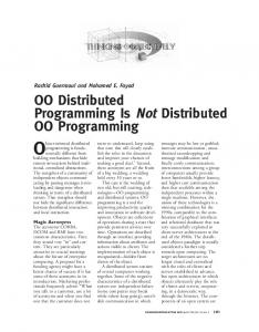
This actor is a software component that wraps interactions with the device drivers. We assume that it does not communicate with any other software component except via its ports. At its input port, it receives a potentially infinite sequence of time-stamped values, called events, in chronological order. The sequence of events is called a signal. The output port produces a time-stamped value for each input event, where the time stamp is strictly greater than that of the input event. The time stamps are values of model time. This software component binds model time to physical time by producing some physical action at the real-time corresponding to the model time of each input event. Thus, the key real-time constraint is that input events must be made available for this software component to process them at a physical time strictly earlier than the time stamp. Otherwise, the component would not be able to produce the physical action at the designated time. Figure 1 shows a distributed DE model to be executed on a two-machine, time-synchronized platform. The dashed boxes divide the model into two parts, one to be executed on each machine. The parts communicate via signal s2 . We assume that events in this signal are sent over a standard network as time-stamped values. The Clock actors in the figure produce time-stamped outputs where the time stamp is some integer multiple of a period p (the period can be different for each clock). Upon receiving an input with time stamp t, the clock actor will produce an output with time stamp np where n is the smallest integer so that np ≥ t. There are no real-time constraints on the inputs or outputs of these actors. The Merge actor has two input ports. It merges the signals on the two input ports in chronological order (perhaps giving priority to one port if input events have identical time stamps). A conservative implementation of this Merge requires that no output with time stamp t be produced until we are sure we have seen all inputs with time stamps less than or equal to t. There are no real-time constraints on the input or output events of the Merge actor.
A
s1
Clock
s3
Device s4 Merge
s2
s5
Display
B
s6
Fig. 1.
Clock
s7
Device
A simple distributed instrumentation example.
The Display actor receives input events in chronological (time-stamped) order and displays them. It also has no realtime constraints. A brute-force implementation of a conservative distributed DE execution of this model would stall execution in platform A at some time stamp t until an event with time stamp t or larger has been seen on signal s2 . Were we to use the Chandy and Misra approach, we would insert null events into s2 to minimize the real-time delay of these stalls. However, we have real-time constraints at the Device actors that will not be met if we use this brute-force technique. Moreover, it is intuitively obvious that such a conservative technique is not necessary. Since the actors communicate only through their ports, there is no risk in processing events in the upper Clock-Device loop ahead of time stamps received on s2 . Our PTIDES technique formalizes this observation using causality analysis. To make this example more concrete, we have in our lab prototype systems provided by Agilent that implement IEEE 1588. These platforms include a Linux host and simple timingprecise I/O hardware. Specifically, one of the facilities is a device driver API where the software can request that the hardware generate a digital clock edge (a voltage level change) at a specified time. After generating this level change, the hardware interrupts the processor, which resets the level to its original value. Our implementation of the Device actor takes input events as specification of when to produce these level changes. That is, it produces a rising edge at physical time equal to the model time of an input event. After receiving an input, it outputs an event with time stamp equal to the physical time at which the level is restored to its original value. Thus, its input time stamps must precede physical time, and its output events are guaranteed to follow physical time. This physical setup makes it easy to measure very precisely the real-time behavior of the system (oscilloscope probes on the digital I/O connectors tell it all). The feedback loops around the two Clock and Device actors ensure that the Device does not get overwhelmed with requests for future level changes. It may not be able to buffer those requests, or it may have a finite buffer. Without the feedback loop, since the ports of the Clock actor have no real-time constraints, there would be nothing to keep it from producing output events much faster than real time. This model is an abstraction of many realistic applications. For example, consider two networked computers controlling cameras pointing at the same scene from different angles. Precise time synchronization allows them to take sequences of pictures simultaneously. Merging two synchronous streams of pictures creates a 4D view for the scene (three physical dimensions and one time). PTIDES programs are discrete-event models constructed as networks of actors, as in the example above. For each actor, we specify a physical host to execute the actor. We also designate a subset of the input ports to be real-time ports. Time-stamped events must be delivered to these ports before physical-time exceeds the time stamp. Each real-time port can optionally also specify a setup time τ , in which case it requires that each input event with time stamp t be received before physical time reaches t − τ . A model is said
4
to be deployable if these constraints can be met for all realtime ports. Causality analysis can reveal whether a model is deployable, as discussed below in section III. The key idea is that events only need to be processed in time-stamp order when they are causally related. We defined formal interfaces to actors that tells us when such causal relationships exist.
p1
p5
p2 A
C
p7
p6 p3
p4 B
p8
Fig. 2.
p9
A composition of actors.
III. R ELEVANT D EPENDENCY Model-time delays play a central role in the existence and uniqueness of discrete-event system behavior. Causality interfaces [16] provide a mechanism that allows us to analyze delay relationships among actors. In this section, we use causality interfaces to derive relevant dependencies among discrete events. Relative dependencies are the key to achieving out of order execution without disobeying the formal semantics of discrete-event specifications. A. Causality Interfaces The interface of actors contains ports on which actors receive or produce events. Each port is associated with a signal. A causality interface declares the dependency that output events have on input events. Formally, a causality interface for an actor a with input ports Pi and output ports Po is a function: δa : Pi × Po → D
(1)
where D is an ordered set with two binary operations ⊕ and ⊗ that are associative and distributive. That is, ∀d1 , d2 , d3 ∈ D, (d1 ⊕ d2 ) ⊕ d3 = d1 ⊕ (d2 ⊕ d3 ) (d1 ⊗ d2 ) ⊗ d3 = d1 ⊗ (d2 ⊗ d3 ) d1 ⊗ (d2 ⊕ d3 ) = (d1 ⊗ d2 ) ⊕ (d1 ⊗ d3 ) (d1 ⊕ d2 ) ⊗ d3 = (d1 ⊗ d3 ) ⊕ (d2 ⊗ d3 )
(2)
In addition, ⊕ is commutative, d1 ⊕ d2 = d2 ⊕ d1 . The ⊗ operator is for serial composition of ports, and the ⊕ operator is for parallel composition. The elements of D are called dependencies, and δa (p1 , p2 ) denotes the dependency that port p2 has on p1 . For discrete-event models, D = R0 ∪ {∞}, ⊕ is the min function, and ⊗ is addition. With these definitions, D is a min-plus algebra [1]. Note that these operators are defined on model time. Given an input port p1 and an output port p2 belonging to an actor a, δa (p1 , p2 ) gives the model-time delay between input events at p1 and resulting output events at p2 . Specifically, if δa (p1 , p2 ) = d, then any event e2 that is produced at p2 as a result of an event e1 at p1 will have time stamp t2 ≥ t1 + δ, where t1 is the time stamp of e1 . For example, a Delay actor with a delay parameter d will produce an event with time stamp t + d at its output p2 given an event with time stamp t at its input p1 , so δDelay (p1 , p2 ) = d. Note that the
causality interface gives the worst case (the smallest possible delay). An actor may produce an event e2 with a larger time stamp, or may produce no event at all in response to e1 , and the actor still conforms with the causality interface. A program is given as a composition of actors, by which we mean a set of actors and connectors linking their ports. Given a composition and the causality interface of each actor, we can determine the dependencies between any two ports in the composition by using ⊗ for serial composition and ⊕ for parallel composition. For example, to determine the dependencies for ports in the composition shown in figure 2, we need to determine the function: δ: P × P → D where P = {p1 , p2 , ...p9 }
(3)
We form a weighted, directed graph G = {P, E}, called the dependency graph, as shown in figure 3, where P is the set of ports in the composition. If p is an input port and p0 is an output port, there is a edge in G between p and p0 if p and p0 belong to the same actor a and δa (p, p0 ) < ∞. In such a case, the weight of the edge is δa (p, p0 ). If p is an output port and p0 is an input port, there is an edge between p and p0 if there is a connector between p and p0 . In this case, the weight of the edge is 0. In all other cases, the weight of an edge would be ∞, but we do not show such edges. Note that this directed graph could by cyclic, and the classical requirement for a DE model to be executable is that the sum (or ⊗) of the edge weights in each cycle be greater than zero [16]. ∀p, p0 ∈ P , to determine the value of δ(p, p0 ), we need to consider all the paths between p and p0 . We combine parallel paths using ⊕ and serial paths using ⊗. In particular, the weight of a path is the sum of the weights of the edges along the path (⊗). The ⊕ operator is minimum, so δ(p, p0 ) is the weight of the path from p to p0 with the smallest weight. For example, δ(p1 , p7 ) is calculated as: δ(p1 , p7 ) =min(ph1 , ph2 ), where ph1 =δA (p1 , p2 ) + 0 + δC (p5 , p7 ), ph2 =δA (p1 , p2 ) + 0 + δB (p3 , p4 ) + 0 + δC (p6 , p7 ) (4) Note that paths with infinite weight in parallel with any path that is shown in our graph would have no effect, which is why we do not show such paths. If there is no path from a port p back to itself, then δ(p, p) = ∞. Note that these dependency values between ports do not tell the whole story. Consider the Merge actor in figure 1. It
5
p7
δ C ( p5 , p7 )
δ C ( p 6 , p7 )
p5
δ C ( p5 , p7 )
p6
p5 & p6
δ A ( p1 , p2 ) p1
Fig. 3. actors.
p4
p4
δ B ( p3 , p4 ) p2
δ C ( p6 , p7 )
δ B ( p3 , p4 ) δ ( p , p ) B 3 9
p9
δ B ( p3 , p9 ) p3
p2
δ B ( p8 , p9 )
p3 & p8
δ B ( p8 , p9 )
p8
A graph for computing the causality interface of a composition of
has two input ports, but when we construct the dependency graph, we will find that there is no path between these ports. However, these ports have an important relationship, noted above. In particular, the Merge actor cannot react to an event at one port with time stamp t until it is sure it has seen all events at the other port with time stamp less than or equal to t. This fact is not captured in the dependencies. To capture it, we define relevant dependencies. B. Relevant Dependency Based on the causality interface of actors, the relevant dependency on any pair (p1 , p2 ) of input ports specifies whether an event at p1 will affect an output signal that may also depend on an event at p2 . The relevant dependency between ports in a composition is calculated in a way similar to the dependency above, but we aggregate some of the ports into equivalence classes. Specifically, considering an individual actor a, two input ports p1 and p2 of a will be “equivalent” if there is an output port that depends on both. Formally, p1 and p2 are equivalent if ∃p ∈ Po , such that δa (p1 , p) < ∞ and δa (p2 , p) < ∞, where Po is the set of output ports of a. For example, in figure 2, assume that both input ports of actor C affect its output port, i.e. that δC (p5 , p7 ) < ∞ and δC (p6 , p7 ) < ∞. Then p5 and p6 are equivalent. In addition, we assume that if any actor has state that is modified or used in reacting to events at more than one input port, then that state is explicitly treated as an output port. Thus, with the above definition, two input ports are equivalent if they are coupled by the same state variables of the actor. For example, in figure 2, port p9 might represent the state of actor B. If both input ports p3 and p8 affect the state, then the dependencies are δB (p3 , p9 ) = δB (p8 , p9 ) = 0, and p3 and p8 are equivalent. We next modify the dependency graph by aggregating ports that are equivalent to create a new graph that we call the relevant dependency graph. Consider the graph in figure 3. Suppose, as above, that p5 and p6 are equivalent and p3 and p8 are equivalent. Then the relevant dependency graph for the model in figure 2 becomes that shown in figure 4. Note that in the relevant dependency graph, there is a path from p8 to p6 that was not present in the dependency graph. Thus, although events at p8 do not affect events at
Fig. 4.
p1
The relevant dependency graph for the model in figure 2.
Clock
p3 p4
Device
p5 p6 Merge
p7
p8
Display
p2
Fig. 5.
The motivating example with names of ports.
p6 (they have no dependency), there is nonetheless a relevant dependency because events at p3 affect events at p9 (which are also affected by events at p8 ) and at p6 . These effects imply an ordering constraint in processing events at p8 and p6 . Below we will show that the relevant dependency induces a partial order on events that defines the constraints on the order in which we can process events. The relevant dependency for a composition of actors is constructed as follows. Let Q be the set of equivalence classes of input ports in a composition. For example, q3,8 = {p3 , p8 } ∈ Q in figure 2. Then, the relevant dependency is a function of the form d: Q × Q → D where for example in figure 2, Q = {q1 , q3,8 , q5,6 } = {{p1 }, {p3 , p8 }, {p5 , p6 }}. Similar to ordinary dependencies, relevant dependencies are calculated by examining weights of the relevant dependency graph. ∀q, q 0 ∈ Q, to determine the value of d(q, q 0 ), we need to consider all the paths between q and q 0 . We again combine parallel paths using ⊕ and serial paths using ⊗. In particular, the weight of a path is the sum of the weights of the edges along the path (⊗). The ⊕ operator is minimum, so d(q, q 0 ) is the weight of the path from q to q 0 with the smallest weight. When the relevant dependency is d(q, q 0 ) = r, r ∈ R0 , this means that any event with time stamp t at any port in q 0 can be processed when all events at ports in q are known up to time stamp t − r. When the relevant dependency is d(q, q 0 ) = ∞, this means that events at any port in q 0 can be processed without knowing anything about events at any port in q. Figure 5 shows a portion of the model in figure 1 and names each port. The causality interface for each actor in the model
6
p1
Clock
p3 p4
Device
p6 Merge p2
Fig. 6.
Delay
p9
e1